Second order entropy diminishing scheme for the euler equations

(1)

HAL Id: hal-00139605

https://hal.archives-ouvertes.fr/hal-00139605

Submitted on 3 Apr 2007

HAL is a multi-disciplinary open access

archive for the deposit and dissemination of

sci-entific research documents, whether they are

pub-lished or not. The documents may come from

teaching and research institutions in France or

abroad, or from public or private research centers.

L’archive ouverte pluridisciplinaire HAL, est

destinée au dépôt et à la diffusion de documents

scientifiques de niveau recherche, publiés ou non,

émanant des établissements d’enseignement et de

recherche français ou étrangers, des laboratoires

publics ou privés.

Second order entropy diminishing scheme for the euler

equations

Frédéric Coquel, Philippe Helluy, Jacques Schneider

To cite this version:

Frédéric Coquel, Philippe Helluy, Jacques Schneider. Second order entropy diminishing scheme for the

euler equations. International Journal for Numerical Methods in Fluids, Wiley, 2006, 50, pp.1029-1061.

�hal-00139605�

(2)

EULER EQUATIONS

F. COQUEL1_{, P. HELLUY}2_{, J. SCHNEIDER}2

Abstract. In several papers of Bouchut, Bourdarias, Perthame and Coquel, Le Floch ([13], [7]...), a general methodology has been developed to construct second order finite volume schemes for hyperbolic systems of conservation laws satisfying the entire family of entropy inequalities. This approach is mainly based on the construction of an entropy diminishing projection. Unfor-tunately, the explicit computation of this projection is not always easy. In the first part of this paper, we carry out this computation in the important case of the Euler equations of gas dynamics. In the second part, we present several numerical applications of the projection in the context of finite volume schemes.

Introduction

In this paper, a methodology to build second order generalized Godunov schemes satisfying all the entropy inequalities is described. Our goal is to adapt the Go-dunov’s original idea, which leads to first order schemes, in order to obtain a second order scheme. The construction is done completely in the case of the Euler equa-tions.

Let us recall that in the classical first order scheme, each step of the time-marching procedure is made up of two stages:

(1) Exact (or high order) resolution of the system of conservation laws starting from the cell averages of the previous time-step. This resolution is per-formed during a short time τ so that the Riemann problems of the two sides of each cell do not interact.

(2) The result of the previous stage is no longer constant in the cells. A projec-tion is then realized in order to recover a piecewise constant approximaprojec-tion. For a first order scheme, the only conservative projection is cell averaging. This description is of course theoretical. In practice, a numerical flux can be asso-ciated to this procedure so that the two stages become transparent in the imple-mentation of the scheme.

The first scheme designed in this way is described by Godunov in [16]. We shall call in the sequel this kind of scheme, based on an exact or approximate Riemann solver, a Godunov scheme. This terminology is developed in the review paper of Harten, Lax and Van Leer [1]. Most of the conservative schemes can be put in this framework as the HLL scheme [1], HLLC scheme of Toro, Spruce and Speares [11], Roe scheme [26], Engquist-Osher scheme [12], kinetic schemes [9], [24], [4], and many others...

The original Godunov scheme has the important property that it respects on the discrete level the decrease of all the Lax entropies of the approximated hyperbolic

1_{Laboratoire d’Analyse Num´}_{erique, Universit´}_{e Paris VI, France.} 2_{Laboratoire ANAM, ISITV, Universit´}_{e de Toulon, France.}

(3)

2 F. COQUEL , P. HELLUY , J. SCHNEIDER

system. This is an important property which is closely linked to the stability of the scheme and with the possibility of non-physical waves if the scheme is not entropic. For example, the HLL, HLLC and Engquist-Osher schemes are entropic whereas the original Roe scheme is not entropic. With a simple modification, it can be made entropic (for example, see the fix of Harten and Hyman [20]).

Another important feature emerging from the construction of the Godunov schemes is that the cell values are high order approximations of the exact mean values. They are also second order approximations of the exact values in the center of the cells. Unfortunately, because they are only first order approximations on the cell sides, an error of order one is committed in the computation of the numerical flux. These remarks have been used to improve the precision of Godunov schemes. The most widespread improvement consists of reconstructing a more precise approxima-tion of the soluapproxima-tion by using cell averages and Taylor expansions. This reconstruc-tion allows one to compute more accurately the fluxes, but has to be corrected by a limitation procedure in order to avoid oscillations or non physical values. The main criterion in these methods is a TVD (Total Variation Diminishing) crite-rion. Many works deal with second order Godunov schemes (we can cite for example the works of Van Leer [22] or Harten [18]) which give good numerical results in var-ious practical computations. Anyway, since the work of Rauch [25] it is well known that the TVD criterions are inadequate in the theoretical study of systems of con-servation laws in higher dimensions. There is no hope to prove convergence results in a general framework with these limitations1.

In this paper, another approach is followed, which is closer to the Godunov’s original idea. On the one hand, we shall consider the resolution of a generalized Riemann problem with piecewise linear (instead of constant) initial data. The solution will then have to be projected back onto a set of piecewise linear functions. On the other hand, in the projection step, we substitute for the TVD criterion a mean en-tropy decreasing criterion which seems more adequate for systems. An important feature is that this stability criterion will be verified for the whole family of entropies of the system. Such an approach has been initiated for scalar conser-vation laws by Bouchut, Bourdarias and Perthame in [13] and has been extended to 2x2 systems of conservation laws and to the 3x3 system of Lagrangian gas dynamics by Coquel and Le Floch in [7]. Our paper deals with the case of the Euler system. The first part is devoted to a mathematical study of the projection stage. The problem can be stated in the following way: the three conservative variables, after the Riemann problem step are, generally speaking, piecewise regular functions in each cell of the finite volume method. The goal of the projection is to recover linear variables in the cells in order to pursue the resolution. Because the mean values of these variables are given by the conservation property, it is sufficient to compute three slopes. The projection can then be seen as the operator which gives these slopes from the original piecewise regular conservatives variables in the cells. It is known that this operator can not be linear. Indeed, it can be proved that a general linear projection (such as the classical L2_{projection) will not always respect}

the positivity of the projected density and pressure. It is of course linked to the fact that there is no second order linear three point scheme which is also TVD for the scalar conservation laws (see [15]). Because we are working on systems we will require that the projection operator is entropic. By entropic, we mean that the mean value in each cell of the entropy of the projection is smaller than the

1_{It should also be noticed that the TVD criterion is limited to cartesian grids in the multi-d} case, even for scalar equations.

(4)

mean entropy of the original conservative variables. It is very interesting that this entropy diminishing property gives also the positivity of the projected variables. This result is proved in remark 2.

Here, we are able to prove the existence of a non-linear projection for the Eu-ler equations and provide explicit formulas. The construction is based on several ingredients:

• First, we recall the theory of second order entropic projections of [13]. This theory is based on the definition of an approximate derivative (Definition 5) and a sufficient condition in order to have an entropic projection (Theorem 1). A very nice feature of this theory is that, when applied to a scalar con-servation law, the entropic projection is very similar to a classical minmod limiter.

• This sufficient condition is not exploitable as is for the Euler system, and it does not give easily an explicit formula for the slopes of the projection. Thus we propose to seek the projection as the composition of two non-linear operators. To build the first operator, we work with special variables (den-sity, momentum and a particular entropy) for which the sufficient condition of Theorem 1 can be computed. We then reduce the first step of the pro-jection to the solution of a triangular set of inequalities (16), (17) and (18) for the three slopes.

• The first operator is not conservative for the energy. The mean value of the projected energy has thus to be corrected. We prove that the correction is still entropy diminishing and thus does not impede the whole process. This fact can also be used by to built simple entropic schemes for the Euler equations based on the intermediate solution of the entropy conservation law.

• Finally, we provide formulas that explicitly solve the fundamental triangular set of inequalities for the slopes. These formulas are summed up in Theorem 2.

The second part of the paper is then devoted to several numerical experiments with the previously constructed projection. One approach could have been to develop a generalized Riemann solver as in [7] for the gas dynamics equations in Lagrangian coordinates. The theory of the generalized Riemann problem can be found, for example, in the papers of Bourgeade, Le Floch, Raviart [5], Ben Artzi, Falcovitz [2]. It is also sketched in the book of Godlewski and Raviart [15]. The problem is that the implementation of this solver is very complex. So we prefer to follow here much simpler approaches. We present two kinds of numerical results:

• The first are obtained with a second order kinetic scheme. We use the Boltz-mann kinetic interpretation of the Euler equations in order to construct an approximate second order Riemann solver. For the computations, we choose a compactly supported Maxwellian proposed by Perthame [24]. But instead of taking a piecewise constant density function in the microscopic scheme, we take a piecewise linear density function. The free transport Boltzmann equation can then be solved exactly. A second order approximate Riemann solver is then obtained by taking the moments of the resulting microscopic solution. After the Boltzmann step, the solution is piecewise polynomial in each cell and can be computed explicitly. We are then in a position to apply the results of the first part of the paper and provide some numerical experiments which validate the whole procedure.

(5)

• The previous construction is quite complicated. So we propose also another approach. We do not try to construct a high order Riemann solver but re-construct a high order approximation of the solution from its cell averages. The cell averages are computed with a standard Godunov flux. Without limitations, the scheme would present oscillations. We then apply the en-tropic projection to the reconstruction in order to evaluate the damping of the oscillations.

We conclude the paper with some comments about possible extensions and appli-cations of the entropic projection.

1. Entropy solution of Euler equations

1.1. Euler equations. In the present paper we focus our attention on the numeri-cal approximation of the discontinuous solutions of the Euler system for polytropic gases. With standard notation, this system reads:

∂tw + ∂xf (w) = 0, t > 0, x ∈ R, (1) w(0, x) = w0(x), where w =   ρ ρu E   , f(w) =   ρu ρu2_{+ p} (E + p)u   , and E = ρε +(ρu) 2 2ρ , p = (γ − 1)ρε, γ > 1.

It is well known that this system is strictly hyperbolic over the phase space Ω = {w ∈ R3, ρ > 0, ρu ∈ R, E −(ρu)

2

2ρ > 0}.

1.2. Entropy condition. Generally, the weak solution of (1) is not unique. As-suming that theoretical results for scalar conservation laws extend to systems, an entropy condition has to be added to the Euler system in order to recover unique-ness.

Definition 1. Let U (w) be a convex function of w, and let F (w) be a function such that the following additional conservation law holds whenever w is a strong solution

∂tU (w) + ∂xF (w) = 0.

(U, F ) is then called a Lax entropy pair for the system (1) (U is the entropy and F the entropy flux).

Definition 2. A weak solution w(t, x) of (1) is an entropy solution if and only if for every entropy pair (U, F ), the following inequality holds

∂tU (w) + ∂xF (w) ≤ 0, t > 0, x ∈ R.

The previous notions have been introduced by Lax in [21] for general systems of conservation laws. The mathematical existence and uniqueness of the entropy so-lution is still an open problem. In this paper this well-posedness result is supposed to hold.

The practical computation of the Lax entropies for the Euler system is given for example (among many others) in the PhD thesis of Croisille [8] or in the book of

(6)

Raviart and Godlewski [14]. It appears that a family of regular entropies can be constructed in the following way: let us introduce the following quantity

S = (ρε)1/γ.

It can be checked that (−S, −uS) is a Lax entropy pair of the Euler system. We now consider the family (U, uU ) defined by

U = ρG(S ρ), where G is a C2_{function on R}+∗ _{such that}

G′

< 0 and G′′

> 0.

It is proved in [8] that this construction gives all the C2 _{entropies of the Euler}

system of the form (U, F ) with F = uU . Another expression of the entropies is given by

U = ρH(ρ S), where H is a C2 _{function on R}+∗ _{such that}

H′

(x) + xH′′

(x) > 0, x ∈ R+∗. 2. Generalized Godunov scheme

The framework of generalized second order Godunov schemes approximating (1) can now be stated.

A time-step τ > 0, and a space-step h > 0 being given, we consider the following discretization in time tn = nτ (n ≥ 0) and space xi = ih (i ∈ Z). The cell i is

defined by Ci=¤xi−1/2, xi+1/2

£ .

We start with an approximation of w(tn, x) at time tn

wn(x) ≈ w(tn, x),

which is supposed to be piecewise linear with

wn(x) = wni + sni(x − xi), ∀x ∈ Ci,

(in the classical Godunov scheme si n = 0).

Remark 1. To be more general, we can also consider another set of variables given by a regular transformation:

φ = φ(w), w ∈ Ω,

and suppose that φ is piecewise linear:

wn(x) = φ−1(φni + dni(x − xi)), ∀x ∈ Ci.

This approach will be developed in the next part.

In order to compute a new wn+1_{(x), two steps are then performed:}

(1) First, the Euler equations and the entropy conditions are exactly solved during a short period of time τ :

∂tv + ∂xf (v) = 0 t > 0, x ∈ R,

∂tU (v) + ∂xF (v) ≤ 0,

v(0, x) = wn(x),

and this is done for all Lax entropy pairs (U, F ). The solution v(τ, x) will be denoted by wn+1,−_{(x) and is generally no longer linear in each cell.}

(7)

(2) wn+1,−_{(x) has to be approximated again by a piecewise linear function. Let}

P1

h be the space of piecewise (per cell) linear functions, then we look for a

(possibly non linear) operator Π : L∞

(R) → Ph1such that

wn+1(x) = Π wn+1,−(x).

Π is also supposed to be a projection in the sense that Πw = w whenever w ∈ P1

h.

In the case of the classical first order Godunov scheme the projection consists simply of cell-averaging Πw(x) = w = 1 h Z Ci w, x ∈ Ci, i ∈ Z.

If the projection is an approximation of order 2 (with respect to h) of wn+1,−_,

then the resulting scheme is of order 2 in space (and of order 1 in time) in the sense of consistency. But good precision will be achieved only under some stability conditions. We shall now describe a possible set of stability conditions.

3. entropy diminishing projection

As mentioned in the introduction, we wish to generalize the Godunov idea to second order schemes. The first step consists of solving exactly (or at least with given precision) generalized Riemann problems between two cells starting from a piecewise linear approximation of the solution. Actually, in order to be more general, we shall consider in each cell the case of an initial condition in a finite dimensional manifold M of regular functions defined on the cell. It is clear that after the exact resolution step, the solution is, generally speaking, no longer in M . A regular approximation in the cell has to be recovered, with the decrease of entropies.

A second order Riemann solver will be constructed later on, and in this part we focus only on the projection step of the Godunov method.

3.1. Second order entropy diminishing projections. Because we are looking for a projection defined locally, i.e. on each cell Ci, we can suppose, for simplicity,

that Ci =]0, 1[. The projection problem can then be presented in the following

abstract setting (introduced in [13], [7]):

Definition 3. Let M be a finite dimension manifold included in C∞

([0, 1], Ω). Let w = (ρ, ρu, E)T _{be an element of L}∞

∩ BV ([0, 1], Ω), and let Π be a (generally non-linear) projection from L∞

∩ BV ([0, 1], Ω) into M which satisfies the following property: for all Lax entropy pairs (U, F ),

(2) Z 1 0 U (Πw(x))dx ≤ Z 1 0 U (w(x))dx.

Such an operator will be denoted as an entropy diminishing projection on M . Let us note that condition (2) implies a conservation property. Indeed, when applied to the following degenerate entropies:

U (w) = ±ρ, U (w) = ±ρu, U (w) = ±E, we get w := Z 1 0 Πw(x)dx = Z 1 0 w(x)dx.

(8)

In the classical Godunov method, M is the set of constant states which are in Ω and the projection is given by

Πw = w.

Inequality (2) then holds thanks to the Jensen inequality. The problem here is that we are looking for an approximation of the function w which is of order two when rescaled to an interval of size h. Let us define precisely this second order property. Definition 4. Let Π be an entropy diminishing projection from L∞

∩ BV ([0, 1], Ω) into M . Let ew be an element of C2_{([0, h], Ω) and w(x) = e}_w(xh), _{x ∈ [0, 1]. After}

projection of w we can define e

Π ew(t) := Πw(t

h), t ∈ [0, h],

then Π is said to be a second order entropy diminishing projection if

(3) ¯¯_¯eΠ ew(t) − ew(t)¯¯_{¯ ≤ λh}2,

where λ is a constant which depends only on the C2 _{norm of e}_w.

As we have seen before, in the case of first order Godunov scheme, the first order entropy diminishing projection is necessarily unique. On the other hand, there exist many second order entropy diminishing projections with various choices of mani-folds M . In the sequel, we recall a general framework which allows the construction of second order entropy diminishing projections. We then use special features of the Euler equations to build a simple explicit projection for this hyperbolic system.

3.2. Pseudo-derivative. We are going to derive a sufficient condition on Π in order to satisfy the very important inequality (2). It is based on the following notion of (what we decided to call) pseudo-derivative which was introduced first by Bouchut, Bourdarias and Perthame in [13] in the case of a scalar equation. It was also studied by Coquel and Le Floch in [7] for systems.

Definition 5. Let w be an element of L∞

∩BV ([0, 1], Ω) . The pseudo-derivative of w is the continuous function N (w) ∈ C(]0, 1[, R3_{) defined by}

N (w)(x) = 2 1 − x Z 1 x w(t)dt − 2 x Z x 0 w(t)dt.

The linear operator N satisfies the following properties:

• For all constants C, N(w + C) = N(w). • If w is regular enough, N(w)(x) = R01ϕ(x, t)w

′_{(t)dt. Where the graph of}

(9)

8 F. COQUEL , P. HELLUY , J. SCHNEIDER ✻ s 0 s 1 ✂✂ ✂✂ ✂✂ ✂✂ ✂✂ ✂✂ ✂ ❏ ❏ ❏ ❏ ❏ ❏ ❏ ❏ ❏ ❏ ❏ ❏ ❏ s x t ϕ(x, t) 2 ✲

• If w is regular, for all x ∈]0, 1[ there is a θ(x) ∈]0, 1[ such that

(4) N (w)(x) = w′ (θ(x)). • If w =R01w(t)dt = 0 then −x(1 − x)₂ N (w)(x) = Z x 0 w(t)dt.

• Finally, if w = R01w(t)dt = 0, the following integration by parts formula

holds _Z 1 0 v(t)w(t)dt = Z 1 0 t(1 − t) 2 N (w)(t)v ′ (t)dt.

A sufficient condition for the decrease of the mean entropy can then be stated. Theorem 1. Let Π be a projection from L∞

∩ BV ([0, 1], Ω) into M. If for all w ∈ L∞

∩ BV ([0, 1], Ω), all x ∈]0, 1[, and all entropies U,

(5) dxΠw · U′′(Πw)(x)(N (w)(x) − dxΠw) ≥ 0,

then, Π is an entropy diminishing projection.

Proof. This is a consequence of the basic convex inequality Z 1 0 U (w) − U(Πw) ≥ Z 1 0 U′ (Πw)(w − Πw) = Z 1 0 U′ (Πw)(w − Πw) (6) + Z 1 0 t(1 − t) 2 dxΠw · U ′′ (Πw)(t)(N (w)(t) − dxΠw)dt. ¤

(10)

At this stage, condition (5) would provide us with a practical definition of Πw if we were studying a scalar equation instead of the Euler system (see [13]). Using the convexity of entropies U , the previous condition reduces to

(7) dxΠw · (N(w)(x) − dxΠw) ≥ 0.

Define the minmod function of a set of reals as minmod E = ¯ ¯ ¯ ¯ ¯ ¯ inf E if E ⊂ R+ sup E if E ⊂ R− 0 otherwise ,

then a possible choice for Πw is the linear function Πw(x) = w + dxΠw(x − 1/2)

where the real number dxΠw is defined by

(8) dxΠw = minmod{N(w)(x), x ∈]0, 1[}.

This defines a second order entropy diminishing projection thanks to property (4). In the case of a system of conservation laws, U′′_{(Πw)(x) are positive definite}

matri-ces which define a metric for all values of x ∈]0, 1[. If that metric was constant then we may define dxΠw as the vector in the convex envelope N◦of {N(w)(x), x ∈]0, 1[}

that minimizes the norm associated to the metric i.e.:

(9) dxΠwT · U′′· dxΠw = min

v∈N◦v

T

· U′′

· v .

But since the metric is changing with x, the practical use of condition (5) is not at all straightforward. The inequality can however be used to establish the existence of a solution (see [7]) and to derive a family of projections that partially (that is to say up to a certain order n) fulfill it (see for an example [7]).

In the next section, we adapt the previous method in order to build an exact second order entropy diminishing projection in the case of the Euler equations.

4. Explicit computation of the projection: Euler case The starting point of the explicit projection procedure is an element

w0= (ρ0, q0= ρ0u0, E0)T ∈ L∞∩ BV ([0, 1], Ω).

In the sequel , we will denote by Π a second order entropy diminishing projection. The projection w2= Πw0 thus belongs to C∞([0, 1], Ω). For practical reasons, w2

will be obtained from an intermediate state, noted w1 = (ρ1, q1 = ρ1u1, E1)T ∈

C∞_{([0, 1], Ω). In other words, w}

1 = Π1w0, and our explicit projection Π is the

composition of two operators Π1 and Π2:

Π = Π2◦ Π1.

Let us first describe operator Π1. We have seen in the introduction that all the

C2 entropies of the Euler system have a rather simple form when expressed as a function of the quantity S = (ρε)1/γ _{. We thus define}

S0= (E0−

1 2ρ0u

2 0)1/γ.

On the other hand, we wish w1 to be C∞. A simple possibility is to set

(10) S1= S0+ dS1(x − 1/2)

(11) ρ1= ρ0+ dρ1(x − 1/2)

(11)

where, as before, z is a notation for the mean value of the quantity z on the interval [0, 1]. The real numbers dS1, dρ1, dq1are to be guessed (and will be defined explicitly

in the sequel).With our choice, the quantities S1, ρ1, q1 are thus linear in the cell

[0, 1] and have the same mean values as S0, ρ0, q0.

Setting (13) w1= (ρ1, q1, E1= 1 2ρ1u 2 1+ S γ 1),

it is clear that w1 is regular but not linear in the cell. It is also clear that, since

S1 = S0, the first projection operator Π1 is not conservative in the sense that, in

general, density and impulsion are conserved but not energy. Thus q1= q0, ρ1= ρ0, E16= E0.

This fact justifies the necessity of a correction w2 = Π2w1, if this approach is

employed, in order to recover the conservation of energy.

The simplest way to obtain w2 is to correct the energy by taking

ρ2= ρ1,

q2= ρ2u2= q1,

E2= E1− E1+ E0,

But with this choice, the operator w0→ w2is not a projection. For this reason, we

prefer to take

(14) E2= 1

2ρ1u

2

1+ (K + S1)γ,

where the constant K should be chosen in such a way that

(15) E2= E0.

We suggest then to define the approximation manifold M by:

Definition 6. _{M is the set of vector functions w = x → (ρ(x), q(x),}q(x)

2

2ρ(x)+ S(x) γ₎

defined on [0, 1] such that the functions ρ, q, and S are linear and such that ∀x ∈ [0, 1], w(x) ∈ Ω (which is equivalent to ∀x ∈ [0, 1], ρ > 0, S > 0).

In other words, according to the notations of Remark 1 (page 5), we have simply set φ = (ρ, ρu, S).

The problem is now to verify that the correction (14) can be done with the decrease

of any entropy U : _Z

U (ρ2, q2, E2) ≤

Z

U (ρ1, q1, E1).

But the convexity of U with respect to the conservative variables gives Z U (ρ1, q1, E1) ≥ Z U (ρ2, q2, E2) + Z _∂U ∂E(w2)(E1− E2). On the other hand, we know that

∂U ∂E(w) = ρG ′ (S ρ) ∂S ∂E, and S = (E −q 2 2ρ) 1/γ ⇒ _∂E∂S = 1 γS 1−γ_{> 0,}

which implies that ∂U_∂E < 0 on the phase space Ω. It is thus natural to require that, E1− E0< 0 on the cell, or, in an equivalent way, that

(12)

Actually, it will be more convenient (and it is possible) to ask a little bit more. We know that the energy is the sum of two terms:

E = q

2

2ρ+ S

γ_,

and we will require the decrease of these two terms separately: (16) Z _q2 1 2ρ1 ≤ Z _q2 0 2ρ0 , and (17) Z C(S1) ≤ Z C(S0) ∀C ∈ C2(R, R), convex.

In order that the global process Π = Π2◦ Π1be entropy decreasing, it is finally

sufficient to require the last family of inequalities (18) Z ρ1H( S1 ρ1)dx ≤ Z ρ0H( S0 ρ0 ), where H is any C2 _{function on R}+∗ _{such that}

H′

(x) + xH′′

(x) > 0, x ∈ R+∗.

Remark 2. Inequality (17) automatically enforces S1> 0 on ]0, 1[. Indeed, consider

a C2_{(R, R) convex function C satisfying}

C(y) = 0 when y ≥ 0,

C(y) > 0 when y < 0,

then, because S0> 0, we have 0 ≤R C(S1) ≤RC(S0) = 0 and then S1> 0. In the

same way, inequality (18) implies that ρ1> 0 if we suppose that S0> 0, S1> 0 and

ρ0> 0. These properties are very important for the numerical approximation of the

Euler equations. They ensure that the resulting second order entropy diminishing scheme is also a positive scheme.

We sum up the previous construction in the following proposition:

Proposition 1. Let w0 = (ρ0, q0 = ρ0u0, E0)T ∈ L∞∩ BV ([0, 1], Ω), and let

w1 = (ρ1, q1= ρ1u1, E1 = 1₂ρ1u21+ S γ

1)T ∈ C∞([0, 1], Ω) where ρ1, q1, and S1 are

linear functions defined by (10), (11), (12). Suppose that the slopes of ρ1, q1, and S1

are computed in order to satisfy (16), (17), (18). Let finally w2 = (ρ1, q1, E2)T ∈

C∞

([0, 1], Ω), where E2 is corrected according to (14) and (15). Then, the

non-linear operator Π : w0→ w2 is an entropy diminishing projection on the manifold

M of definition 6 (on page 10).

The construction of an entropy diminishing second order projection is now reduced to the computation of three slopes dS1, dρ1, and dq1 satisfying inequalities (16),

(17) and (18). The important fact is that we have now to solve a triangular set of inequalities. In practice, we will have first to find a dS1 satisfying (17). Then our

choice of S1will be inserted in (18) in order to get dρ1. Then, knowing S1 and ρ1,

we are in a position to solve (16) and compute q1.

The computation of S1 is quite simple if we apply the computations leading to

formula (8). We thus propose

(19) dS1= minmod {N(S0)(x), x ∈ [0, 1]} .

(13)

Lemma 1. Let ρ0 and S0 be two positive functions in L∞∩ BV ([0, 1], R). Let ρ1

and S1 be two positive and linear functions defined on [0, 1]:

(20) S1= S0+ dS1(x − 1/2),

(21) ρ1= ρ0+ dρ1(x − 1/2).

Then, a sufficient condition on the slope dρ1 in order to have (18) is that the

following inequality holds on [0, 1]:

(22) α · µ_S 1 S0 (S0N (ρ0) − ρ0N (S0)) − S0+ N (S0)(x − 1/2) S0 α ¶ ≥ 0, where α is defined by α = S0dρ1− ρ0dS1.

Proof. It is easy to check that (ρ, S) → ρH(S/ρ) is a convex function. Thus, using Theorem 1, a sufficient condition in order to have (18) is

(dρ1, dS1) Ã ₁ −ρ1 S1 −ρ1 S1 ³ ρ1 S1 ´2 ! µ N (ρ0) − dρ1 N (S0) − dS1 ¶ ≥ 0, or (S1dρ1− ρ1dS1)(S1N (ρ0) − ρ1N (S0) − (S1dρ1− ρ1dS1)) ≥ 0.

using (20) and (21), and thanks to basic computations, we find (22). ¤ The slope dq1 is computed in the same spirit.

Lemma 2. Let q0and ρ0be two functions in L∞∩ BV ([0, 1], R), with ρ0> 0. Let

q1 and ρ1 be two linear functions defined on [0, 1], with ρ1> 0.

(23) q1= q0+ dq1(x − 1/2),

ρ1= ρ0+ dρ1(x − 1/2).

Then, a sufficient condition on the slope dq1 in order to have (16) is that the

following inequality holds on [0, 1]

(24) β · µ_ρ 1 ρ0 (ρ0N (q0) − q0N (ρ0)) − ρ0+ N (ρ0)(x − 1/2) ρ0 β ¶ ≥ 0, where β is defined by β = (ρ0dq1− q0dρ1).

The next theorem is devoted to the practical computation of the slopes dS1, dρ1, dq1

in order to solve inequalities (16), (17), (18) and in order to maintain the second order property.

Theorem 2. With the previous notations, consider:

α = S0dρ1− ρ0dS1, β = (ρ0dq1− q0dρ1), gα(x) = S0+ N (S0)(x)(x − 1/2) S0 , gβ(x) = ρ0+ N (ρ0)(x)(x − 1/2) ρ0 , hα(x) = S1 S0 (S0N (ρ0)(x)−ρ0N (S0)(x)) and hβ(x) = ρ1 ρ0 (ρ0N (q0)(x)−q0N (ρ0)(x)).

Then, if dS1 is defined by (19) and if α and β are defined by

1 α =      maxx∈[0,1]hgαα(x)(x) if hα> 0 minx∈[0,1] g_hα_α(x)_(x) if hα< 0 ∞ otherwise ,

(14)

1 β =      maxx∈[0,1]_hgβ_β(x)_(x) if hβ> 0 minx∈[0,1]ghββ(x)(x) if hβ< 0 ∞ otherwise ,

then, ρ1, S1, q1 are second order approximations of respectively ρ0, S0, q0, and

inequalities (17), (22), (24) are satisfied. In other words, with this choice of slopes, Π is a second order entropy diminishing projection.

Proof. The case of dS1has already been treated before. The inequality to solve for

α is

α(hα(x) − αgα(x)) ≥ 0.

α = 0 is a solution, but in order to achieve second order, α has to be a first order approximation of hα(x). Thus, we can assume that α and hα have the same

signs. Then, suppose that hα(x) > 0 for all x ∈ [0, 1]. If α > 0, we have to solve

1/α ≥ gα(x)/hα(x), x ∈ [0, 1]. We thus take 1/α = max[0,1]ghαα(x)(x) > 0. In the same

way, if hα(x) < 0 we choose 1/α = min[0,1]_hgα_α(x)_(x) < 0. Finally, if hα takes positive

and negative values on [0, 1], we take α = 0. The computation of β is completely

similar. ¤

5. First application: a second order Boltzmann scheme

5.1. An approximate Riemann solver based on a kinetic interpretation. In this part, a possible computation of wn+1,− _{is presented. For practical reasons,}

we shall not use a classical Riemann solver, but instead, a resolution step based on the kinetic interpretation of the Euler equations. The kinetic interpretation that we will describe below has been proposed by Perthame in [24]. His model has the property of being entropy diminishing for one particular entropy (see [24]) and not necessarily for the other entropies. For simplicity, it will be exposed in the case γ = 3, where the computations are easier, but can be extented to other values of γ. Actually, it would be better to use the more recent model of Bouchut as described into [3], which is entropy diminishing for all entropies.

Let us describe the original kinetic interpretation of Perthame. For this purpose, we introduce the following function (called in the sequel generalized Maxwellian).

(25) Mw(v) = ρ 2√6εY ( v − u √ 6ε ), where:

• Y is the characteristic function of [−1, 1]: Y (t) =

½

1 if |t| < 1 0 if |t| ≥ 1 . • v is the microscopic speed.

• w =   ρuρ

E 

 is the macroscopic state of the gas. It is straightforward to check that

Z v=+∞ v=−∞ Mw(v)   v1 v2_/2   dv = w. Let us now set

(15)

It is also easy to check that (26)

Z v=+∞

v=−∞

∂tm + v∂xm = ∂tw + ∂xf (w).

This fact leads to a numerical resolution known as a Boltzmann scheme. Many papers have been published on this subject. Without pretending to be exhaustive, we can cite for example the works of Deshpande [9], Bourdel, Mazet, Delorme and Croisille [4]. All these works are based on the physical Maxwellian. Each time step of a Boltzmann scheme is made of two substeps.

• Free transport step: wn_{(x) being given, the following evolution problem is}

solved during a time step:

∂tg + v∂xg = 0, 0 ≤ t ≤ τ,

g(0, x, v) = Mwn_(x)(v).

(27)

• Collision step: from the solution at time t = τ, a new macroscopic state is recovered wn+1,−(x) = Z v=+∞ v=−∞ g(τ, x, v)K(v)dv. where K(v) =   1v v2/2  

It is important here to point out that the Boltzmann solver is only an approximate Riemann solver. This is due to the fact that during the free transport procedure (27) the equality

m(t, x, v) = g(t, x, v)

does not hold (the microscopic state is not a generalized Maxwellian). The collision step acts as a relaxation of the microscopic state to a Maxwellian state. Of course this solver tends to an exact solver when τ → 0.

On the other hand, despite its simplicity, this approach leads to very tedious com-putations for wn+1,−_{. Therefore, we propose the following simplification: in the}

free transport step (27), we replace the initial condition by its linear interpolation on each cell f (0, x, v) = x − xi−1/2 h Mwi,r(v) + xi+1/2− x h Mwi,l(v) for x ∈ Ci , where wi,r= wni + h 2s n i and wi,l= wni − h 2s n i .

It must be noticed that this approximation is conservative but unfortunately, it is also necessarily entropy increasing because we replace a Maxwellian state (which corresponds to a minimum of entropy) at each point of the cell by a linear approx-imation.

5.2. Computation of the approximate second-order Riemann solver. Let x ∈ Ci, we have:

wn+1,−(x) =

Z +∞

(16)

Consider then the speed vmin (respectively vmax) at which a particle in xi+1/2

(respectively xi−1/2) at time t = 0 reaches x at time t = τ

vmin = x − x i+1/2 τ < 0, vmax = x − x i−1/2 τ > 0.

The time step τ is supposed to be smaller than hv∗_{, where v}∗ _{is greater than the}

biggest support of all the generalized Maxwellians plus the maximal speed of the flow. Thanks to this CFL condition, the computation of wn+1,−_{(x) can then be}

split into three parts: a contribution from the left cell Ci−1, the right cell Ci+1,

and the middle cell Ci:

wn+1,−_{(x) = A} l+ Am+ Ar Al = Z +∞ v=vmax ·_{x − vτ − x} i−3/2 h Mwi−1,r(v) + xi−1/2− x + vτ h Mwi−1,l(v) ¸ K(v)dv, Ar = Z vmin v=−∞ · x − vτ − xi+1/2 h Mwi+1,r(v) + xi+3/2− x + vτ h Mwi+1,l(v) ¸ K(v)dv, Am = Z vmax v=vmin ·_{x − vτ − x} i−1/2 h Mwi,r(v) + xi+1/2− x + vτ h Mwi,l(v) ¸ K(v)dv. A more detailed expression of Al, Ar, Amis given in Appendix 1. It can be checked

that wn+1,− _{is piecewise polynomial of degree ≤ 4 on each cell. The number of}

pieces is ≤ 22.

5.3. Numerical results. For the numerical results that are presented in this sec-tion, we decided to compute exactly wn+1,− _{given by the kinetic Riemann solver.}

This is done thanks to a C++ class of piecewise polynomial functions. It appears then that Sn+1,−_{is not, in general, piecewise polynomial. We thus had to construct}

a piecewise polynomial approximation ˜S of Sn+1,−_{. This is done with a}

Tcheby-chev interpolation with 3 points on each piece of regularity of wn+1,−. Then N (ρ), N (q), and N ( ˜S) can be computed exactly. The final limitation procedure has been performed numerically with a sampling of the functions we wanted to maximize or minimize on each cell.

We were able to verify that our projection operator acts at least as a classical minmod limiter. Indeed, the numerical results appear to be precise and present no oscillation on a 200 cells mesh.

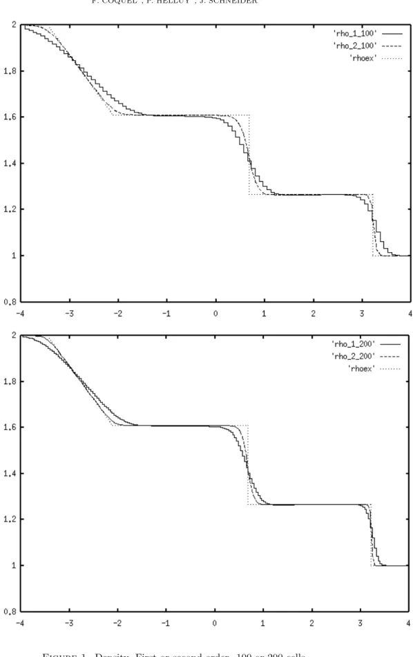
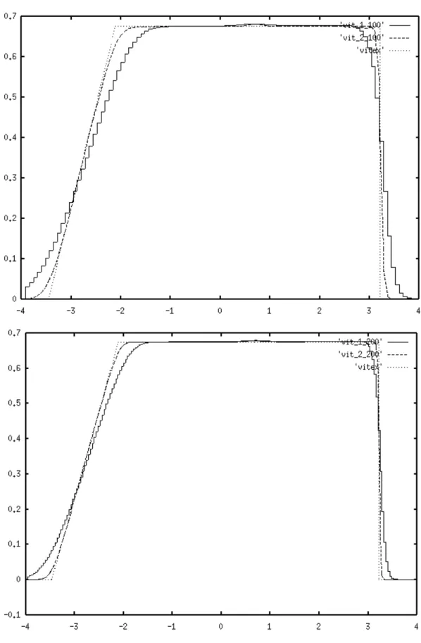
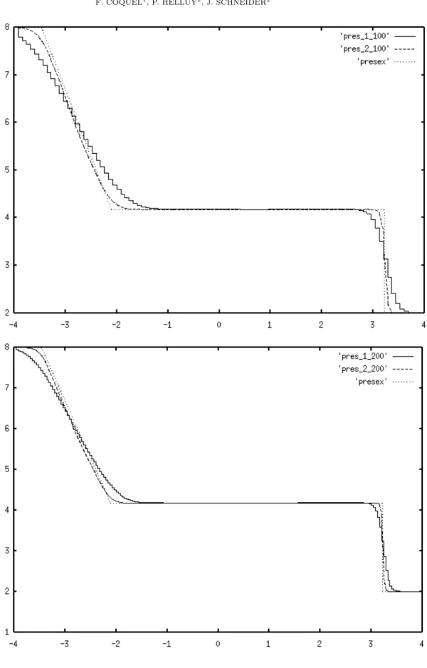
We tested the scheme on the classical case of a shock tube problem with the following initial data:

Variable Left state Right state

Density ρL= 2 ρR= 1

Velocity uL= 0 uR= 0

Pressure pL= 8 pR= 2

In the Figures 1, 2 and 3 a comparison is made between the first and the second order schemes with 100 or 200 cells. The results are given at time t = 1. In the case of the first order solution, the real (piecewise constant) mathematical solution has been plotted. Density, velocity and pressure are successively presented. With a mesh refinement, oscillations start to appear. The phenomenon can be observed with a classical MUSCL scheme. This is due to the fact that the scheme is only first order in time.

(17)

The complexity of the scheme leaded us to abandon this approach. The next section is thus devoted to a more tractable application of the entropic projection.

6. Second application: Mean value approach

In this part, we envisage a simpler approach than the kinetic approach. We first build a polynomial interpolation of the solution, starting from cell averages, as in Harten’s ENO schemes [19]. We use an interpolation without upwinding or limitation in order to evaluate the effect of the entropic projection.

More precisely, suppose that we know the mean value wn

i of the solution at time n

in the cell Ci. A second order extension of the Godunov scheme reads

(28) wn+1_i = wn i − τ h(f n+1/2 i+1/2 − f n+1/2 i−1/2).

The flux at interface i + 1/2 and time n + 1/2 is of the form (29) f_i+1/2n+1/2= f (R(w_i+1/2,−n+1/2 , wn+1/2_i+1/2,+)).

The quantity R(wL, wR) denotes the solution of the first order exact Riemann

problem at the interface between wLand wR. The quantity wi+1/2,−is the value of

the reconstructed solution in the cell i at time n + 1/2 and at the interface i + 1/2. The choice wi+1/2,−= wni corresponds to the classical first order scheme. We focus

now on the cell i. For simplicity, we suppose that Ci =]0, 1[.

The first step is to construct a high order approximation of w from the cell averages. We thus suppose, with the notations of Section 4, that ρ0, q0 and S0 are second

order polynomials in ]0, 1[. We also suppose that the reconstruction is conservative (30) Z j+1 j w0(x)dx = wni+j, j = −1, 0, 1, with (31) w0(x) = (ρ0(x), q0(x), q2 0(x) 2ρ0(x) + S0(x)γ)T.

It is known that the resulting interpolation is not necessarily positive for the density and the pressure, even if all the mean values are positive. So we propose in Appendix 2 a simple procedure to correct the interpolation, if necessary.

Because ρ0, q0 and S0 are now second order polynomials, the computations

de-scribed in Theorem 1 become almost explicit. It is then possible to compute the limited variables ρ1, q1 and S1, the energy correction described in (14) and then

the fluxes at cell interfaces. The second order in time is achieved with the Hancock method. It uses the space slope estimate to compute a time derivative estimate thanks to the conservation laws: wt= −f(w)x. The time derivative estimate

per-mits then to compute the approximation of w at time n + 1/2.

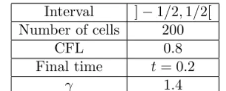
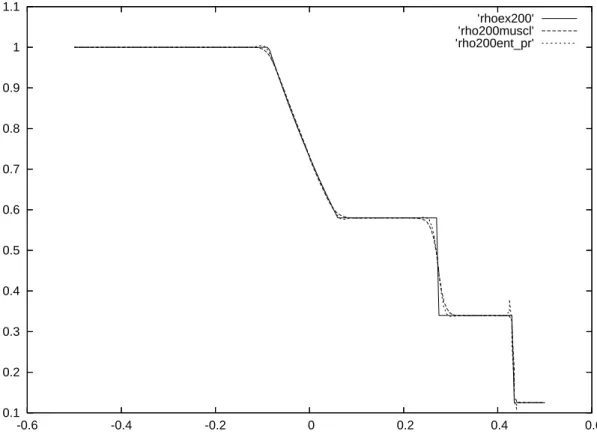
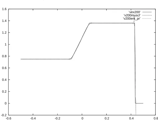
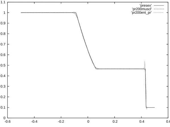
We have tested the scheme on the Riemann problem whose data are given in ta-bles 1 and 2. This case is chosen in the book of Toro [11]. It presents a sonic rarefaction wave and a shock. We compare in Figures 4, 5 and 6 the results of the reconstruction-limitation scheme with a standard MUSCL-Hancock scheme (de-scribed in [11]). We observe a slight improvement of the precision in the contact discontinuity, but also small overshoots and undershoots in the right shock. With-out the correction described in Appendix 2 the computation would have not ended. It is necessary only on one cell in the first time step and only for the reconstruction of the density ρ near the contact discontinuity.

(18)

Density ρL= 1 ρR= 0.125

Velocity uL= 0.75 uR= 0

Pressure pL= 1 pR= 0.1

Table 1. Data of the Riemann problem.

Interval ] − 1/2, 1/2[

Number of cells 200

CFL 0.8

Final time t = 0.2

γ 1.4

Table 2. Computation characteristics.

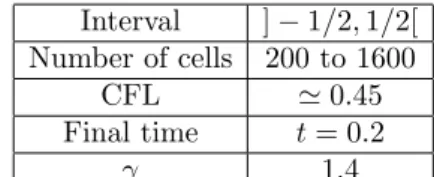
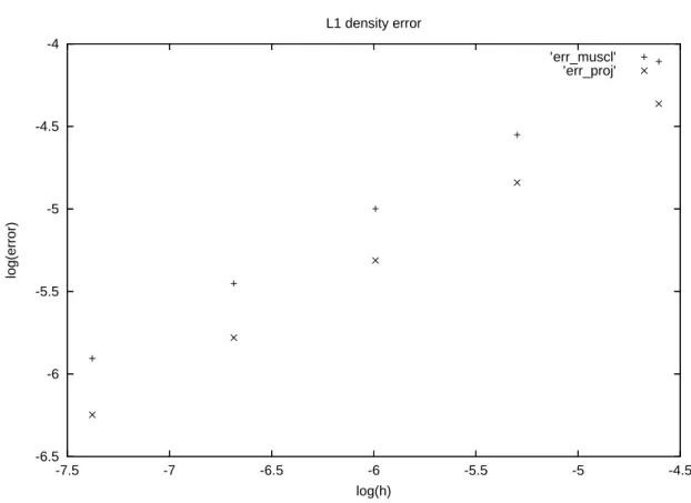
In the next numerical experiment, we evaluate the rate of convergence in the L1

norm (for density ρ) of the reconstruction-limitation scheme and compared it in Figure 7 and Table 3 with the standard MUSCL-Hancock scheme. The rate is com-puted for a simple contact discontinuity whose values are given in Table 4. The characteristics of this computation are summed up in Table 5. We observe that the projection scheme is more precise than the MUSCL scheme, but the asymp-totic rates of convergence seems to be approximately the same. Recall that, for a simple contact discontinuity, the standard MUSCL ”second order” scheme has a convergence rate of 2/3 ≃ 0.66666.

ln(h) ln(error) MUSCL ln(error) proj. rate MUSCL rate proj.

-4.60517 -4.10716 -4.36288 -

--5.29832 -4.55118 -4.84035 0.64058 0.68884

-5.99146 -4.99951 -5.31210 0.64681 0.68060

-6.68461 -5.45112 -5.77950 0.65153 0.67431

-7.37776 -5.90507 -6.24700 0.65491 0.67446

Table 3. Convergence test, contact discontinuity.

Density ρL= 2 ρR= 1

Velocity uL= 1 uR= 1

Pressure pL= 1 pR= 1

Table 4. Contact discontinuity.

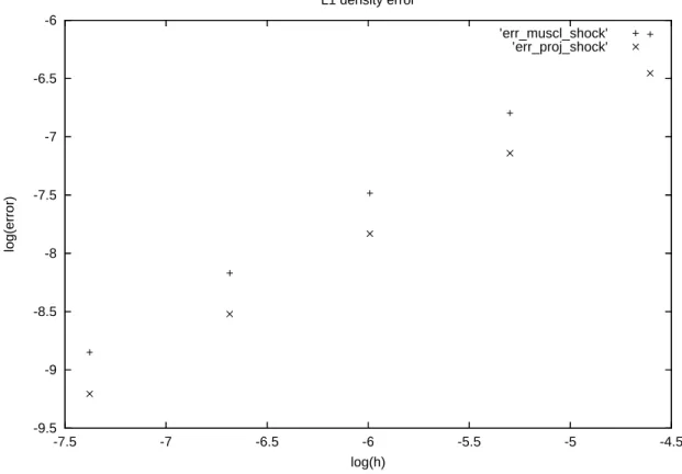
In the last numerical experiment, we evaluate the rate of convergence in the L1_norm

(for density ρ) of the reconstruction-limitation scheme and compared it in Figure 8 and Table 6 with the standard MUSCL-Hancock scheme. The rate is computed for a simple shock whose values are given in Table 7. The characteristics of this computation are summed up in Table 8. We observe that the projection scheme is more precise than the MUSCL scheme, but the asymptotic rates of convergence seem to be approximately the same. Recall that, for a simple shock, the standard MUSCL ”second order” scheme has a convergence rate of 1.

The program we used for the numerical results of this section can be downloaded at

(19)

18 F. COQUEL , P. HELLUY , J. SCHNEIDER Interval ] − 1/2, 1/2[ Number of cells 200 to 1600 CFL ≃ 0.45 Final time t = 0.2 γ 1.4

Table 5. Computation characteristics, contact.

ln(h) ln(error) MUSCL ln(error) proj. rate MUSCL rate proj.

-4.60517 -6.12021 -6.45422 -

--5.29832 -6.79584 -7.14075 0.97472 0.99045

-5.99146 -7.48411 -7.83202 0.99297 0.99730

-6.68461 -8.17001 -8.52117 0.98954 0.99423

-7.37776 -8.84886 -9.20612 0.97937 0.98817

Table 6. Convergence test, shock.

Density ρL= 1 ρR= 3/4

Velocity uL= 0 uR= −1/3

Pressure pL= 1 pR= 2/3

Table 7. Shock wave of velocity 1.

Interval ] − 1/2, 1/2[ Number of cells 200 to 1600

CFL ≃ 0.58

Final time t = 0.2

γ 1.4

Table 8. Computation characteristics, shock.

http://helluy/entropy/index.html 7. Conclusion

In this paper, we have proposed a second order generalization of the Godunov scheme for the Euler equations. In the first part, we have built a second order entropic projection with explicit formulas. In the second part, we have numerically tested the projection. Because it is difficult to construct an exact second order Riemann solver, we had to simplify the theoretical approach. We proposed two applications: the slope limitation applied to an approximate kinetic Riemann solver and the slope limitation applied to a polynomial reconstruction with cell averages. Our approach is rigorous and gives a clear justification to the slope limitation procedure.

Many questions still remain. For example:

(1) Is it possible to extend the scheme to higher dimensions? (2) Can we improve the efficiency of the computation?

(3) Is it possible to extend the method to more general Equation Of State (EOS) than the perfect gas EOS ?

(20)

The answer to the first question is yes. It can be done with at least two methods. The first method, which is the simplest could be to use an alternate direction method. Then the scheme is limited to cartesian grids. Another way would be to extend Theorem 1 to triangles or quadrilaterals. We do not know if the computation of the practical projection remains possible.

The answer to the second question is certainly yes. But we do not know if it is possible to find a simpler computation without abandoning an exact entropy decrease. By relaxing the exact entropy decrease or approximating the formula of Theorem 2, some schemes have already been designed for the Lagrangian equations in [7].

The answer to the third question is: maybe yes. The main ingredient in the pre-sented construction is the existence of an entropy whose hessian is degenerated. For a given pressure EOS

(32) p = p(τ = 1/ρ, ε),

the Lax entropies of the associated Euler equations are constructed, as described in [17], from the concave solutions s(τ, ε) of

(33) ∂s

∂τ − p ∂s ∂ε = 0.

The Lax entropies are then U = −ρs. The general concave solutions of (33) are of the form s = A(s0) where A is a function with monotony and convexity properties,

and s0 a particular solution. If the hessian of s0 is degenerated, maybe that the

previous construction can be generalized.

We would like to end this presentation by insisting on the fact that the second order entropic projection can be used as a slope limiter for other numerical methods. The Galerkin discontinous method (see [23], [6], [10]...) could be a candidate for such a limiter. Indeed in this method a piecewise polynomial approximation at each time step has to be limited in order to avoid spurious oscillations.

Appendix 1: computations for the Boltzmann scheme

We start with Am: Am = x − x i−1/2 h Z vmax v=vmin Mwi,r(v)K(v)dv −τ_h Z vmax v=vmin Mwi,r(v)vK(v)dv +xi+1/2− x h Z vmax v=vmin Mwi,l(v)K(v)dv +τ h Z vmax v=vmin Mwi,l(v)vK(v)dv

(21)

20 F. COQUEL , P. HELLUY , J. SCHNEIDER Am = x − x i−1/2 h ρi,r 2p6εi,r   v2v_/2 v3_/6  

min(vmax,ui,r+√6εi,r)

max(vmin,ui,r−√6εi,r)

−τ_h ρi,r 2p6εi,r   v2_/2 v3_/3 v4_/8  

min(vmax,ui,r+√6εi,r)

max(vmin,ui,r−√6εi,r)

+xi+1/2− x h ρi,l 2p6εi,l   v2v_/2 v3_/6  

min(vmax,ui,l+√6εi,l)

max(vmin,ui,l−√6εi,l)

+τ h ρi,l 2p6εi,l   v2_/2 v3_/3 v4_/8  

min(vmax,ui,l+√6εi,l)

max(vmin,ui,l−√6εi,l)

In the same way:

Al = x − x i−3/2 h ρi−1,r 2p6εi−1,r   v2v_/2 v3_/6   ui−1,r+√6εi−1,r

max(vmax,ui−1,r−√6εi−1,r)

−τ_h ρi−1,r 2p6εi−1,r   v2_/2 v3_/3 v4_/8   ui−1,r+√6εi−1,r

max(vmax,ui−1,r−√6εi−1,r)

+xi−1/2− x h ρi−1,l 2p6εi−1,l   v2v_/2 v3_/6   ui−1,l+√6εi−1,l

max(vmax,ui−1,l−√6εi−1,l)

+τ h ρi−1,l 2p6εi−1,l   v 2_/2 v3_/3 v4_/8   ui−1,l+√6εi−1,l

max(vmax,ui−1,l−√6εi−1,l)

and Ar = x − x i+1/2 h ρi+1,r 2p6εi+1,r   v2v_/2 v3_/6  

min(vmin,ui+1,r+√6εi+1,r)

ui+1,r−√6εi+1,r −_hτ ρi+1,r 2p6εi+1,r   v2_/2 v3_/3 v4_/8  

min(vmin,ui+1,r+√6εi+1,r)

ui+1,r−√6εi+1,r +xi+3/2− x h ρi+1,l 2p6εi+1,l   v2v_/2 v3_/6  

min(vmin,ui+1,l+√6εi+1,l)

ui+1,l−√6εi+1,l +τ h ρi+1,l 2p6εi+1,l   v 2_/2 v3_/3 v4_/8  

min(vmin,ui+1,l+√6εi+1,l)

(22)

It is easy to check that wn+1,− _{is piecewise polynomial and continuous on each cell.}

For instance, the practical computation of a term like A =   v2v_/2 v3_/6   min(vmax,V ) max(vmin,v) where v < V, gives A =   V2_{/2 − v}V − v2_/2 V3_{/6 − v}3_/6 

 if vmin< v and vmax> V, i.e. x ∈

¤ V τ + xi−1/2, vτ + xi+1/2 £ A =   V2V − v_{/2 − v}min2 min/2 V3_{/6 − v}3 min/6 

 if vmin> v and vmax> V, i.e. x ∈¤vτ + xi+1/2, V τ + xi+1/2

£ A =   v2vmax− v max/2 − v2/2 v3 max/6 − v3/6 

 if vmin< v and vmax< V, i.e. x ∈¤vτ + xi−1/2, V τ + xi−1/2

£ A = 0 if x > V τ + xi+1/2 or x < vτ + xi−1/2

Remark: by the CFL condition the inequality V τ +xi−1/2< vτ +xi+1/2necessarily

holds.

Appendix 2: positive mean value interpolation

This appendix is devoted to an algorithm in order to avoid negative values in the interpolation process. In all the numerical tests that we presented it was necessary to activate this correction only on a few cells. This method can be interesting for other purposes.

For this, we consider a scalar non-negative function f defined on the interval [−1, 2]. We know the mean values of f on the sub-intervals Ii = [i − 1, i], i = 0, 1, 2

(34) fi=

Z i

i−1f (t)dt ≥ 0.

A classical interpolation would be to find a second order polynomial P satisfying

(35) fi=

Z i i−1

P (t)dt,

but it is known that this interpolation can be negative in some point in the interval [0, 1], even if the three mean values fi are positive. Instead, we will consider a

constrained optimization problem. We consider a base (Pi) of the second order

polynomials satisfyingR_I

iPj= δij where δij is the Kronecker symbol.

(36) P1(x) = −x2+ x + 5 6, P0(x) = x2 2 − x + 1 3, P2(x) = x2 2 − 1 6. The polynomial P is searched under the form

(23)

In this way, the mean values of P on [i − 1, i] are gifor i = 0, 1, 2. The conservation

property imposes

(38) g1= f1.

We then consider the functional J(P ) = 1₂¡(g0− f0)2+ (g2− f2)2¢. We solve the

optimization problem: find P ≥ 0 such that g1 = f1 and J(P ) is minimal. Note

that if the interpolation polynomial defined in (35) is non-negative then it solves the minimization problem and then J(P ) = 0.

Consider the Lagrangian L(P, µ) = J(P )− < µ, P >, where µ is in the set M1,+_of

positive bounded measures on [0, 1]. The optimization problem is equivalent to

(39) inf g0,g1,g2 g1=f1 sup µ∈M1,+ L(P, µ). The optimality condition classically reads

g0= f0+ < µ, P >,

g2= f2+ < µ, P >,

∀x ∈ [0, 1] , µ(x)P (x) = 0.

But a second order polynomial has at most two roots. This means that µ is a linear combination of at most two Dirac masses. Due to the fact that P has to be non-negative, we can then distinguish the following cases:

(1) P is positive, then g0= f0, f1= g1 and g2= f2.

(2) P is positive in ]0, 1] and P (0) = 0 then f0 = g0+ µ0P0(0), f1 = g1 and

f2= g2.

(3) P is positive in [0, 1[ and P (1) = 0 then f2 = g2+ µ2P2(1), f1 = g1 and

f0= g0.

(4) P is positive in ]0, 1[ and P (0) = P (1) = 0 then f0 = g0+ µ0P0(0), f2 =

g2+ µ2P2(1) and f1= g1.

(5) P is positive in [0, 1] − x0, with x0 ∈]0, 1[. Then, f0 = g0+ µ0P0(x0),

f2= g2+ µ0P2(x0), f1= g1, P (x0) = 0, P′(x0) = 0.

Due to the positivity of P , case (4) never happens. The algorithm to compute P is then the following.

First, we have necessarily f1= g1. Then the following cases are considered:

(1) If g1 ≥ 1/2(g0 + g2)) take f0 = g0, f1 = g1, f2 = g2. The resulting

polynomial is concave and >0;

(2) if g1≤ 1/2(g0+g2)), try f0= g0, f1= g1, f2= g2. The resulting polynomial

is convex. It is solution if P (0) ≥ 0, P′

(0) ≥ 0 or P (1) ≥ 0, P′

(1) ≤ 0. (3) if g1< 1/2(g0+g2)) and 7/2g1−1/2g2≥ 0 and µ0= 3/2g2−15/2g1−3g0≥ 0

then the solution is given by f0= g0+ µ0/3, f2= g2;

(4) if g1< 1/2(g0+g2)) and 7/2g1−1/2g0≥ 0 and µ2= 3/2g0−15/2g1−3g2≥ 0

then the solution is given by f0= g0, f2= g2+ µ2/3;

(5) Finally, if g1< 1/2(g0+g2)) in all the other cases, solve f0= g0+µ0P0(x0),

f2= g2+ µ0P2(x0), f1= g1, P (x0) = 0, P′(x0) = 0 for x0 and µ0.

The algorithm, written in Maple and C++ languages, can be downloaded and tested at

http://helluy/entropy/index.html .

(24)

References

[1] P.D. Lax A. Harten and B. Van Leer. On upstream differencing and godunov-type schemes for hyperbolic conservation laws. SIAM Review, vol. 25:35–61, 1983.

[2] Matania Ben-Artzi and Joseph Falcovitz. An upwind second-order scheme for compressible duct flows. SIAM J. Sci. Statist. Comput., 7(3):744–768, 1986.

[3] F. Bouchut. Construction of BGK models with a family of kinetic entropies for a given system of conservation laws. J. Statist. Phys., 95(1-2):113–170, 1999.

[4] Fran¸coise Bourdel, Jean-Pierre Croisille, Philippe Delorme, and Pierre-Alain Mazet. On the approximation of K-diagonalizable hyperbolic systems by finite elements. Applications to the Euler equations and to gaseous mixtures. Rech. A´erospat., (5):15–34, 1989.

[5] A. Bourgeade, Ph. LeFloch, and P.-A. Raviart. An asymptotic expansion for the solution of the generalized Riemann problem. II. Application to the equations of gas dynamics. Ann. Inst. H. Poincar´e Anal. Non Lin´eaire, 6(6):437–480, 1989.

[6] Bernardo Cockburn, San Yih Lin, and Chi-Wang Shu. TVB Runge-Kutta local projection discontinuous Galerkin finite element method for conservation laws. III. One-dimensional systems. J. Comput. Phys., 84(1):90–113, 1989.

[7] F. Coquel and P. LeFloch. An entropy satisfying muscl scheme for systems of conservation laws. Numerische Mathematik, 74(01):1–34, 1996.

[8] J. P. Croisille. Contribution à l’étude théorique et à l’approximation par éléments finis du système hyperbolique de la dynamique des gaz multidimensionnelle et multiespèces. PhD thesis, Université Paris VI, 1991.

[9] S. Deshpande and J. Mandal. Kinetic theory based new upwind methods for inviscid com-pressible flows. In Proceedings of Euromekh Colloquium 224 on Kinetic Theory Aspects of Evaporation/Condensation Phenomena, volume 19, pages 3, 6, 9, 32–38, 1988.

[10] V. Dolejˇs´ı, M. Feistauer, and C. Schwab. A finite volume discontinuous Galerkin scheme for nonlinear convection-diffusion problems. Calcolo, 39(1):1–40, 2002.

[11] M. Spruce E. F. Toro and W. Speares. Restoration of the contact surface in the hll-riemann solver. Shock Waves, 4:25–34, 1994.

[12] Bj¨orn Engquist and Stanley Osher. One-sided difference approximations for nonlinear con-servation laws. Math. Comp., 36(154):321–351, 1981.

[13] C. Bourdarias F. Bouchut and B. Perthame. A muscl method satisfying all the numerical entropy inequalities. Math. of Comp., 65(216):1439–1461, 1996.

[14] E. Godlewski and P. A. Raviart. Numerical approximation of hyperbolic systems of conser-vation laws. Springer, 1996.

[15] Edwige Godlewski and Pierre-Arnaud Raviart. Numerical approximation of hyperbolic sys-tems of conservation laws, volume 118 of Applied Mathematical Sciences. Springer-Verlag, New York, 1996.

[16] S. K. Godunov. A difference scheme for numerical computation of discontinuous solutions of equations of fluids mechanics. Math Sbornik, n 47:271–306, 1959.

[17] A. Harten, P. D. Lax, C. D. Levermore, and W. J. Morokoff. Convex entropies and hyper-bolicity for general Euler equations. SIAM J. Numer. Anal., 35(6):2117–2127, 1998. [18] A. Harten and S. Osher. Uniformly high order accurate nonoscillatory schemes, i. SIAM

Journal on Numerical Analysis, 24:279–309, 1982.

[19] Ami Harten. ENO schemes with subcell resolution. J. Comput. Phys., 83(1):148–184, 1989. [20] Ami Harten and James M. Hyman. Self-adjusting grid methods for one-dimensional

hyper-bolic conservation laws. J. Comput. Phys., 50(2):235–269, 1983.

[21] P.D. Lax. Hyperbolic systems of conservation laws and the mathematical theory of shock waves. In CBMS Regional Conf. Ser. In Appl. Math. 11, Philadelphia, 1972. SIAM. [22] B. Van Leer. Towards the ultimate conservative difference scheme. a second order sequel to

the godunov’s method. Journal of Computational Physics, 32:101–136, 1979.

[23] P. Lesaint and P.-A. Raviart. On a finite element method for solving the neutron transport equation. In Mathematical aspects of finite elements in partial differential equations (Proc. Sympos., Math. Res. Center, Univ. Wisconsin, Madison, Wis., 1974), pages 89–123. Publi-cation No. 33. Math. Res. Center, Univ. of Wisconsin-Madison, Academic Press, New York, 1974.

[24] B. Perthame. Boltzmann type schemes for gas dynamics and the entropy property. SIAM Journal on Numerical Analysis, vol. 27:1405–1421, 1990.

[25] Jeffrey Rauch. BV estimates fail for most quasilinear hyperbolic systems in dimensions greater than one. Comm. Math. Phys., 106(3):481–484, 1986.

[26] P. L. Roe. Approximate Riemann solvers, parameter vectors, and difference schemes. J. Com-put. Phys., 43(2):357–372, 1981.

(25)

(26)

(27)

(28)

0.1 0.2 0.3 0.4 0.5 0.6 0.7 0.8 0.9 1 1.1 -0.6 -0.4 -0.2 0 0.2 0.4 0.6 ’rhoex200’ ’rho200muscl’ ’rho200ent_pr’

(29)

28 F. COQUEL , P. HELLUY , J. SCHNEIDER -0.2 0 0.2 0.4 0.6 0.8 1 1.2 1.4 1.6 -0.6 -0.4 -0.2 0 0.2 0.4 0.6 ’vex200’ ’v200muscl’ ’v200ent_pr’

(30)

0 0.1 0.2 0.3 0.4 0.5 0.6 0.7 0.8 0.9 1 1.1 -0.6 -0.4 -0.2 0 0.2 0.4 0.6 ’presex’ ’pr200muscl’ ’pr200ent_pr’

(31)

30 F. COQUEL , P. HELLUY , J. SCHNEIDER -6.5 -6 -5.5 -5 -4.5 -4 -7.5 -7 -6.5 -6 -5.5 -5 -4.5 log(error) log(h) L1 density error ’err_muscl’ ’err_proj’

Figure 7. Comparison entropic scheme-MUSCL Hancock scheme. Rate of convergence for a contact discontinuity.

(32)

-9.5 -9 -8.5 -8 -7.5 -7 -6.5 -6 -7.5 -7 -6.5 -6 -5.5 -5 -4.5 log(error) log(h) L1 density error ’err_muscl_shock’ ’err_proj_shock’

Figure 8. Comparison entropic scheme-MUSCL Hancock scheme. Rate of convergence for a shock.