A simple second order cartesian scheme for compressible Euler flows
Texte intégral
Figure


![Figure 7: Comparison of the L 2 accuracy of the classical symmetry technique, the ghost-cell CCST method [11] and the present method.](https://thumb-eu.123doks.com/thumbv2/123doknet/12423126.333958/16.892.185.692.778.997/figure-comparison-accuracy-classical-symmetry-technique-method-present.webp)


Documents relatifs
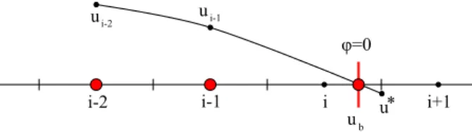
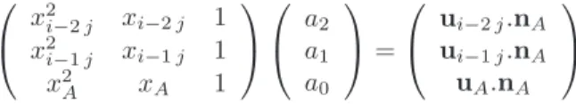
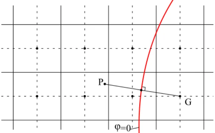
This method is based on a classical finite volume approach, but the values used to compute the fluxes at the cell interfaces near the solid boundary are determined so to satisfy
Two-grid discretizations have been widely applied to linear and non-linear elliptic boundary value problems: J. These methods have been extended to the steady Navier-Stokes
Theorem 4.1 (Unconditional stability of the scheme) Let us suppose that the discrete heat diffusion operator satisfies the monotonicity property (3.20), that the equation of
In this section, we build a pressure correction numerical scheme for the solution of compressible barotropic Navier-Stokes equations (1), based on the low order non-conforming
Danchin: On the well-posedness of the full compressible Navier-Stokes system in critical Besov spaces, Journal of Differential Equations, (2015).
Keywords: incompressible Navier-Stokes equations, vector BGK schemes, flux vector splitting, low Mach number limit, discrete entropy inequality, cell Reynolds number, lattice
Danchin: Well-posedness in critical spaces for barotropic viscous fluids with truly nonconstant density, Communications in Partial Differential Equations, 32 , 1373–1397 (2007).
For Navier-Stokes equations, either compressible or incompressible, several types of methods provide an order two accuracy in space, global as well as local (near the interface):
