HAL Id: tel-01247499
https://tel.archives-ouvertes.fr/tel-01247499
Submitted on 4 Jan 2016
HAL is a multi-disciplinary open access
archive for the deposit and dissemination of sci-entific research documents, whether they are pub-lished or not. The documents may come from teaching and research institutions in France or abroad, or from public or private research centers.
L’archive ouverte pluridisciplinaire HAL, est destinée au dépôt et à la diffusion de documents scientifiques de niveau recherche, publiés ou non, émanant des établissements d’enseignement et de recherche français ou étrangers, des laboratoires publics ou privés.
Design and construction
Hung Dang Phuc
To cite this version:
Hung Dang Phuc. Development of portable low field NMR magnet : Design and construction. Medical Imaging. INSA de Lyon, 2015. English. �NNT : 2015ISAL0007�. �tel-01247499�
Thèse
Développement d’aimant bas champ pour RMN Portable:
Conception et construction
Présentée devantL’Institut National des Sciences Appliquées de Lyon
Pour obtenirLe Grade de Docteur
École Doctorale : Électronique, Électrotechnique, Automatique Spécialité : Micro et nanotechnologies, Instrumentation Laboratoire : CREATIS, CNRS UMR 5220 – INSERM U1044 – INSA Lyon ParDANG PHUC Hung
Soutenue le 29 janvier 2015 devant la commission d’examen JURY :Directeur de thèse: Mme. Latifa FAKRI-BOUCHET, Maitre de Conférences, HDR. CREATIS, INSA de Lyon.
Co-directeurs: M. Patrick POULICHET, Professeur Associé, ESIEE Paris.
M. Huan PHAN DINH, Professeur Associé, Institut Polytechnique d’Ho Chi Minh Ville, Vietnam.
Rapporteurs: M. Kosai RAOOF, Professeur des Universités, LAUM, ENSIM, Université du Maine. M. Jean-Paul YONNET, Directeur de recherches CNRS, G2Elab, ENSE3, INP,
Grenoble.
Examinateurs: M. Daniel BARBIER, Professeur des Universités, INL, INSA de Lyon. Invité: M. Abdennasser FAKRI, Professeur Associé, ESIEE Paris
CHIM E.E E2M EDI INFOM Matér ME ScS *ScSo : H MIE http Sec : Bat B 3e eta Insa .A. ELE AUT http: Secr eea@ M2 EVO MIC http: Insa ISS INTE http Sec : Insa MATHS INFO http Sec : Bat B 3e eta infom riaux MAT http Secré PM : Bat. Ed.m GA MEC CIV http Secr PM : Bat. meg So ScSo http Sec : Brigi Insa istoire, Géograph ://www.edchim :Renée EL MEL Blaise Pascal age : R. GOURDON ECTRONIQUE TOMATIQUE //edeea.ec-lyon étariat : M.C. H @ec-lyon.fr OLUTION, EC CROBIOLOGI //e2m2.universi : H. CHARLES ERDISCIPLIN ://www.ediss‐ : : M. LAGARD ORMATIQUE ://infomaths.un :Renée EL MEL Blaise Pascal age maths@univ-lyo TERIAUX DE ://ed34.univer étariat : M. LAB 71.70 –Fax : 8 Saint Exupéry materiaux@insa CANIQUE, EN VIL, ACOUSTI ://mega.univer étariat : M. LAB : 71.70 –Fax : 8 Saint Exupéry [email protected] o* ://recherche.u : Viviane POLSIN tte DUBOIS : J.Y. TOUSSAIN hie, Aménagemen mie-lyon.fr LHEM N E, ELECTROT n.fr HAVGOUDOUK COSYSTEME, IE, MODELIS ite-lyon.fr S NAIRE SCIEN ‐lyon.fr DE E ET MATHEM niv-lyon1.fr LHEM on1.fr LYON site‐lyon.fr BOUNE 87.12 ‐lyon.fr NERGETIQUE IQUE rsite-lyon.fr BOUNE 87.12 r niv‐lyon2.fr/scs NELLI NT nt, Urbanisme, Ar TECHNIQUE, KIAN SATION NCES-SANTE MATIQUES E, GENIE so/ rchéologie, Scienc Universit Bât ESCP 43 bd du 69622 VI Tél : 04.7 directeur M. Gérar Ecole Cen 36 avenu 69134 EC Tél : 04.7 Gerard.sc Mme Gud CNRS UM Universit Bât Forel 43 bd du 69622 VI Tél : 06.0 e2m2@ u Mme Em INSERM U Bâtiment 11 avenu 696621 V Tél : 04.7 Emmanu Mme Sylv LIRIS – IN Bat Blaise 7 avenue 69622 VI Tél : 04.7 Sylvie.ca M. Jean‐Y INSA de L MATEIS Bâtiment 7 avenue 69621 VI Tél : 04.7 Jean‐yves M. Philip INSA de L Laborato Bâtiment 25 bis av 69621 VI Tél :04.72 Philippe. M. OBAD Universit 86 rue Pa 69365 LY Tél : 04.7 Lionel.Ob ce politique, Socio té de Lyon – Col E 11 novembre 1 LLEURBANNE C 72.43 13 95 r@edchimie‐lyo rd SCORLETTI ntrale de Lyon ue Guy de Collon CULLY 72.18 60.97 Fax corletti@ec‐lyo drun BORNETTE MR 5023 LEHNA té Claude Berna 11 novembre 1 LLEURBANNE C 07.53.89.13 univ‐lyon1.fr mmanuelle CAN U1060, CarMeN t IMBL ue Jean Capelle Villeurbanne 72.68.49.09 Fax elle.canet@uni vie CALABRETTO NSA de Lyon e Pascal e Jean Capelle LLEURBANNE C 72. 43. 80. 46 Fa alabretto@insa Yves BUFFIERE Lyon t Saint Exupéry e Jean Capelle LLEURBANNE C 72.43 83 18 Fax s.buffiere@insa pe BOISSE Lyon oire LAMCOS t Jacquard enue Jean Cape LLEURBANNE C 2 .43.71.70 Fax boisse@insa‐lyo DIA Lionel té Lyon 2 asteur YON Cedex 07 78.77.23.86 Fax badia@univ‐lyo ologie, Anthropol llège Doctoral 1918 Cedex on.fr ngue : 04 78 43 37 1 on.fr E A ard Lyon 1 1918 Cédex NET‐SOULAS N lab, Univ. Lyon INSA de Lyon :04 72 68 49 16 iv‐lyon1.fr O Cedex ax 04 72 43 16 8 a‐lyon.fr Cedex 04 72 43 85 28 a‐lyon.fr elle Cedex x : 04 72 43 72 3 on.fr x : 04.37.28.04.4 on2.fr ogie 7 n 1 6 87 37 48
Acknowledgements
I would never have been able to finish my dissertation without the guidance of my committee members, help from friends, and support from responsible peoples in laboratory CREATIS.
I would like to express my deepest gratitude to my supervisor, Mrs. Latifa FAKR-BOUCHET, for her excellent guidance, caring, patience, and providing me with an excellent atmosphere for doing research. I would like to thank my co-supervisor, Mr. Patrick POULICHET, who let me experience the research of portable NMR devices, patiently corrected my writing. I would also like to thank another co-supervisor, Mr. PHAN DINH Huan, who gave me valuable suggestions for my works. Special thank goes to Mr. Christian Jardin, who introduced me to study in France and Mr. Abdennasser FAKRI for his help during I had studied in ESIEE, Paris.
I would like to be thankful to Mr. Kosai RAOOF and Mr. Jean-Paul YONNET, who accepted to be reviewers and gave many useful comments for my work. I would like to express my thankfulness to Mr. Daniel BARBIER, who accepted to be president of the jury.
Finally, I would also like to thank my parents, young sisters. They were always supporting me and encouraging me with their best wishes. This thesis will be dedicated for my grandmother, who passed away during I had studied in France.
Les travaux menés au cours de cette thèse ont porté essentiellement sur le développement d’un aimant pour système de Résonance Magnétique Nucléaire (RMN) portable : conception, modélisation et simulation puis réalisation et validation.
Chapitre 1 : Introduction à la RMN
Nous présentons dans ce premier chapitre les bases nécessaires pour comprendre les points clés de l’expérience de RMN. Depuis sa découverte en 1945, la résonance magnétique nucléaire (RMN) est devenue un outil précieux pour la physique, la chimie, la biologie et la médecine. La RMN se décline sous forme de deux techniques d’investigation non-invasives spectroscopie de résonance magnétique nucléaire (SRM) et l'imagerie par résonance magnétique (IRM).
Ces techniques exploitent le fait que certains noyaux atomiques possèdent un moment cinétique intrinsèque « le spin ». Placés dans un champ magnétique statique B0, les moments magnétiques associés aux spins s’orientent parallèlement et antiparallèlement au champ B0 selon deux niveaux d’énergie tout en maintenant leurs mouvements de précession.
Le phénomène de la RMN consiste à faire passer les spins d’un niveau d’énergie à l’autre. Pour ce faire on a recours à une impulsion de champ radiofréquence B1, un champ électromagnétique qui oscille à la même fréquence de précession des spins. Les noyaux absorbent l’énergie radiofréquence qu’ils restituent sous forme d’onde donnant naissance, selon le cas à un spectre ou une image RMN dont les caractéristiques dépendent du type de noyau et de son environnement chimique.
A l’arrêt de l’impulsion radiofréquence, les spins continuent leur précession autour d’un axe perpendiculaire au champ B0, puis l’aimantation globale (résultante de tous les moments magnétiques) revient à son état d’équilibre. Le temps de retour à l’équilibre est appelé temps de relaxation longitudinale T1. Il est caractéristique des tissus et dépend des molécules en présence. Il existe aussi un temps de relaxation dit T2, temps de relaxation transversale correspondant à la constante de temps de décroissance de la tension électrique correspondante à l’onde restituée, lors de la détection, par les spins. T2 dépend essentiellement de la nature de l’atome et de son environnement magnétique immédiat.
A l’état macroscopique le phénomène de précession et de relaxation est décrit par les équations de Bloch :
0 1/ 2 0
0 0 1/ 1
La RMN portable permet d’accéder à l’enveloppe du signal et ainsi à l’amplitude qui permet d’extrapoler la quantité de proton en présence. Les constantes de temps T1 et T2 donnent des informations sur les interactions entre - par exemple - les noyaux d’hydrogène et leur environnement.
Dans ce chapitre nous avons aussi discuté les techniques de mesure des temps de relaxation T1 et T2, plus particulièrement la mesure de T2. L’intérêt est que cette mesure peut être effectuée en champ magnétique non uniforme en utilisant plusieurs impulsions créant ainsi un train d’échos. Il existe deux techniques bien connues pour la mesurer du T2 : Échos de spin ou Echo de Hahn et la séquence d'impulsions CPMG.
Dans ce chapitre, nous avons terminé notre revue des bases de RMN par des considérations concernant l'influence de l'homogénéité du champ magnétique sur la spectroscopie RMN. Il est nécessaire d’effectuer les expériences de RMN dans un champ magnétique B0 le plus homogène possible. L'homogénéité de B0 reste un critère important dont il faut tenir compte lors de la conception d'un dispositif de RMN portable.
Chapitre 2 : Conception de système de RMN Portable : Etat de l’art
Ce deuxième chapitre est un récapitulatif de l'état de l'art concernant les appareils de RMN portables. Le développement de ces dispositifs portables est exposé de manière exhaustive afin d'avoir un aperçu de ce domaine de recherche et pouvoir choisir la solution la plus adéquate pour nos applications.
La question qui se pose est pourquoi une RMN portable ? Alors que la plupart des chercheurs s’orientent vers des champs de plus en plus élevés et des protocoles de mesure de plus en plus complexes. En effet, les systèmes de RMN classiques produisent des champs magnétiques très intenses homogènes et stables avec cependant des aimants volumineux, coûteux en maintenance et en énergie. De plus, ils limitent la taille maximale de l’échantillon à leurs dimensions internes, alors qu’un système de RMN portable - dans sa configuration ex-situ par exemple - peut être positionné à la surface des objets d’étude sans limitation de taille.
extrêmes. Un exemple significatif est les systèmes de la société Magritek (Nouvelle-Zélande), pour l’analyse des changements des propriétés mécaniques des glaces arctiques avec le réchauffement climatique.
Le développement de la technologie des aimants permanents tels que des aimants de « terre rare » a permis aux chercheurs de les utiliser pour des applications RMN. Ces aimants peuvent produire un champ fort et homogène, deux critères importants pour les exigences expérimentales en RMN. Autres caractéristiques attrayantes d'aimants permanents sont évidemment l'absence de la source d'énergie électrique extérieure et pas de maintenance. Ainsi, ils remplissent les conditions pour la conception de dispositifs portables RMN.
Les dispositifs RMN portables sont divisés en deux groupes en raison des applications visées. Un premier groupe appelé ex-situ avec des échantillons d’étude placés à l'extérieur de l'aimant. Un second groupe appelé in situ où les échantillons sont analysés à l'intérieur de l'aimant.
Les appareils de RMN portables ex-situ ont une configuration simple avec le volume sensible (région d'intérêt: ROI) à proximité de leur surface. Ces systèmes sont appropriés pour des investigations de surface. Ainsi, ils peuvent être utilisés pour des objets aux dimensions illimitées. Les aimants in situ ont, quant à eux, la particularité de renforcer le champ en leur centre et par conséquent nul en dehors du champ de la structure. Dans ce cas, leur champ magnétique est homogène à l'intérieur de la structure en comparaison avec aimants ex situ. Un autre avantage d'aimants in situ, il est moins sensible aux influences environnementales externes en raison du confinement du champ.
Dans ce chapitre, nous nous sommes intéressés aussi aux techniques d’optimisation de l’homogénéité du champ magnétique et leurs applications aux aimants portables. Fondamentalement, deux méthodes répandues ont été utilisées pour augmenter l’homogénéité du champ magnétique. La première méthode est l'optimisation de l'écart entre les deux anneaux de la configuration. Cependant, cette méthode n’améliore pas suffisamment l'homogénéité pour spectroscopie. Le « Shim » est la seconde méthode c’est la plus utilisée pour augmenter l'homogénéité du champ magnétique des appareils de RMN en général et les RMN portables en particulier. La technique du « Shim » est non seulement utilisée pour augmenter l'homogénéité du champ magnétique, mais aussi utilisé pour compenser l'hétérogénéité causée par les imperfections du matériau, les tolérances de fabrication et les imprécisions d’assemblage.
Ce chapitre est consacré à la discussion sur les propriétés des matériaux magnétiques et les méthodes numériques.
Les propriétés des matériaux magnétiques ont été discutées dans la première section de ce chapitre. Nous avons examiné différentes familles de matériaux magnétiques les plus utilisés ces quinze dernières années afin de choisir le matériau le plus approprié pour notre application.
Les méthodes numériques de simulation mises en œuvre ont également été détaillées dans ce chapitre. Nous présentons le calcul de champ magnétique sur la base de la méthode des éléments finis, sous-jacente au logiciel ANSYS (nous avons utilisé ce logiciel pour les calculs et la simulation). En outre, les matériaux de l'élément de la bibliothèque d'éléments d'ANSYS sont décrits dans notre procédure de simulation.
Les méthodes numériques et la simulation jouent un rôle important à la conception de l'aimant et le processus d'optimisation. La géométrie de l'instrument doit être définie par les utilisateurs et les paramètres spécifiques peuvent être alors optimisés. Les stratégies analytiques fournissent des solutions précises pour la distribution du champ magnétique dans la région d'intérêt (ROI) et le profil de champ magnétique. Dans la littérature, il existe différentes méthodes numériques que nous avons décrites aussi dans ce chapitre.
Les éléments utilisés pour la simulation dans la bibliothèque de logiciel ANSYS ont été décrits. Selon le problème à résoudre, les utilisateurs peuvent choisir les éléments appropriés. Par exemple, l'élément PLANE53 est utilisé pour la simulation 2-D tandis que l'élément SOLID98 est considéré pour des solutions 3-D. Dans ce travail, deux éléments sont utilisés pour la simulation. L'élément PLANE13 et SOLID97 est respectivement utilisé pour la 2-D et 3-D simulation.
Nous nous sommes intéressés aussi aux matériaux permanents, matériaux qui maintiennent une aimantation en l’absence de champ extérieur. Ces matériaux sont souvent anisotropes (ils admettent un axe d’aimantation) et suivent une courbe d’hystérésis après leur première aimantation. Dans ce chapitre, nous discutons, par ailleurs, certains de leurs paramètres essentiels à ce travail. Ainsi plusieurs propriétés magnétiques initiales d'un matériau peuvent être déterminées:
‐ La rémanence d'un matériau (Br) mesurée en Tesla (T) est sa capacité à maintenir une magnétisation lorsqu'un champ magnétique externe est retiré après avoir atteint la saturation, avec Br = μ0Mr où Mr est l’aimantation rémanente.
l'intensité du champ magnétique extérieur H opposé à l’aimantation rémanente, nécessaire pour que l’induction magnétique dans le matériau soit annulée (B 0H M
).
Il existe une variété de matériaux pour aimants permanents, nous avons donné un bref résumé sur des matériaux de qualité généralement utilisés dans la fabrication d'aimants, leurs avantages et désavantages respectifs. Plus particulièrement les aimants permanents utilisant un matériau moderne tel que le NdFeB, que nous avons retenu pour sa meilleure rémanence et coercivité ainsi que son prix bas.
Chapitre 4 : Conception, construction de poids léger RMN portables de type Halbach de barres identiques aimants
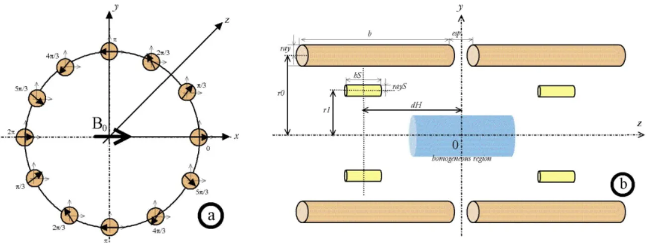
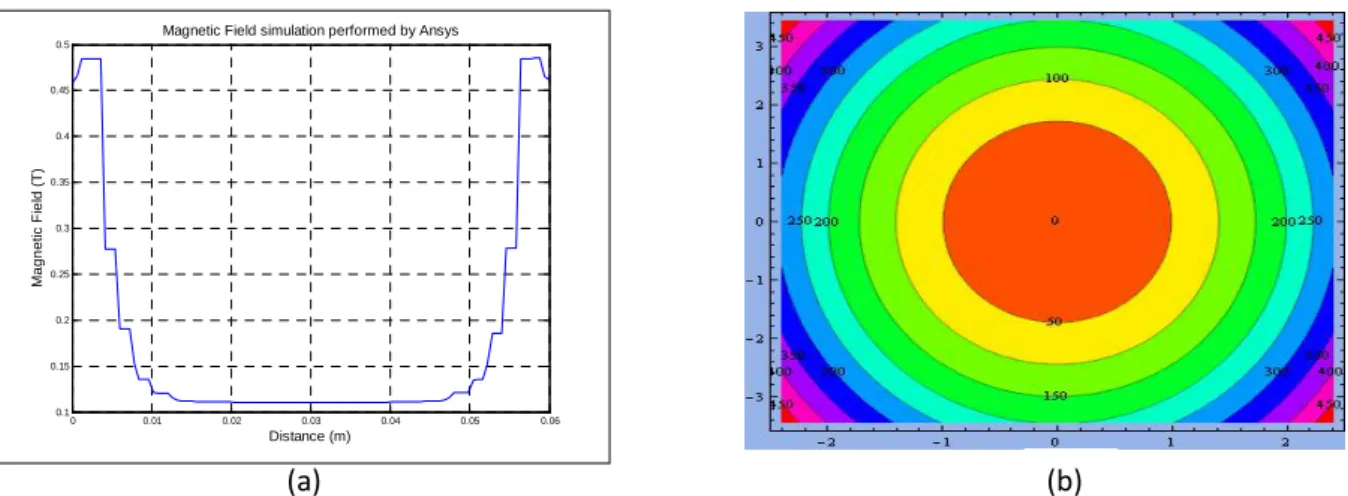
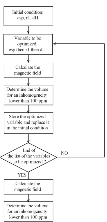
Ce chapitre présentera une conception simple pour dispositif de RMN portable. La configuration est basée sur le type Halbach. Il a deux anneaux principaux alignés pour compenser le champ magnétique à l'extérieur des anneaux. Chaque anneau est composé de 12 aimants identiques de forme cylindrique. Pour prédire les propriétés de cette configuration, l’intensité du champ magnétique et l'homogénéité sont calculées et simulées par deux logiciels qui sont ANSYS et RADIA. Ces deux méthodes sont complémentaire: RADIA est utilisé pour l'optimisation et de simulation. ANSYS est utilisé pour la vérification des résultats obtenus par RADIA. Les résultats obtenus par les deux logiciels sont en bonne corrélation à la fois pour la simulation et l'optimisation. La valeur maximale de B0 calculée avec RADIA est 0,103 T alors que la valeur correspondante dérivée de l'analyse ANSYS est de 0,11 T. La différence de calcul entre RADIA et ANSYS est 6,79%. Cette différence a été discutée dans ce chapitre. Une nouvelle méthode de shim pour augmenter l'homogénéité et corriger les imperfections du champ B0 a été aussi introduite. La position des aimants de shim a fait l’objet d’une optimisation avec le logiciel RADIA et vérifié par le logiciel ANSYS.
Sur la base de ces résultats, nous avons réalisé un nouveau prototype. Ses propriétés ont été vérifiées par simulation et mesurée également. Ce prototype est constitué de deux anneaux de 12 aimants. Ces aimants sont placés en cercle de 30 mm de rayon et insérés dans douze trous de deux couronnes en aluminium. Les deux anneaux du prototype, fixés par des vis sur les couronnes en aluminium, peuvent coulisser sur trois tiges pour obtenir la position souhaitée des aimants.
limite de sensibilité de 10-4 T dans une gamme variant de 0 à 0,299 T. Le Micro-positionneur Signatone S-926 est utilisé pour contrôler le mouvement de la sonde dans les trois directions. La résolution est de 254 µm « per knob révolution ». Les différences constatées entre la mesure et la simulation sont expliquées à la fin de ce chapitre.
Chapitre 5: Modélisation et conception de la configuration Mandhalas pour des applications biomédicales et agro-alimentaire.
Un autre aimant basé sur la configuration Mandhalas (Magnet Arrangement for Novel Discrete
Halbach Layout) a fait l’objet d’une étude comparative, portant sur deux configurations utilisant
des aimants de formes circulaires et de formes carrés, effectuée par simulation 2D (sur la base de trois critères: la masse, l'homogénéité et l'intensité du champ magnétique). Les Mandhalas fabriqués à partir d’aimants circulaires permettent d’avoir de meilleurs résultats (0.32 T, 178 ppm). Sur la base du résultat de la simulation 2D, la configuration avec 16 aimants permanents de formes circulaires a été choisie pour la construction de notre prototype. La simulation 3D a permis d’évaluer le système dans sa globalité.
Tenant compte des résultats obtenus, un système de shim passif a été aussi utilisé dans ce cas et a permis l’augmentation de la zone d'homogénéité de manière significative. Les résultats de l'optimisation indiquent que dans l'axe longitudinal, la région homogène s’étend sur 2,5 fois en comparaison de celle sans le système de shim. L'homogénéité du champ magnétique dans un volume cylindrique de diamètre de 40 mm et de 50 mm de longueur est de 178 ppm au lieu de 638 ppm dans le cas de la configuration sans les aimants de shim, soit une valeur d’homogénéité supérieure d’un facteur 3,5.
Partant des résultats de simulation, nous avons conçu un prototype d'environ 20 kg de poids total. Cet aimant de table génère un champ magnétique de 0,32 T et offre une homogénéité de 178 ppm dans un volume sensible de 40 mm de diamètre et de 50 mm de longueur.
Conclusion et perspective
En raison de nos objectifs d’applications, nous avons choisi un aimant in situ de configuration de type Halbach pour son homogénéité et sa capacité à confiner le champ à l'intérieur. Les avantages et les inconvénients des matériaux magnétiques ont été analysés. Sur la base de ces analyses, nous avons constaté que la famille des aimants NdFeB est adaptée à nos travaux. Ce matériau
retenu en raison de son prix élevé (30% à 40% plus cher que le NdFeB).
Les méthodes numériques existantes ont été également examinées afin de définir la meilleure solution pour nos travaux de simulation et d'optimisation. Nous avons choisi la méthode des éléments finis, procédure sous-jacente de nombreux logiciels.
Les calculs et les simulations sont principalement basés sur ANSYS, dont les résultats ont été confrontés et vérifiés par les résultats obtenus avec le logiciel RADIA. Le principe de calcul ANSYS est basé sur la méthode des éléments finis tandis que celui de RADIA repose sur des méthodes d’intégrales aux limites. Les résultats sont en parfaite concordance aussi bien pour l'homogénéité que pour l'optimisation. Cependant, l'intensité du champ magnétique est différente entre les deux logiciels en raison du maillage choisi. Nous avons également utilisé Matlab pour les différents tracés.
Les mesures ont été effectuées avec l'gaussmètre Hirst GM08 avec une limite de sensibilité 10-4T. Le micro positionneur Signatone S-926 est utilisé pour contrôler le mouvement de la sonde dans les trois directions de l’espace.
A partir des résultats de la simulation, nous avons réalisé un prototype compact et léger avec 24 aimants « tige » identiques. Notre prototype a deux anneaux; chaque anneau est composé de 12 aimants. Chaque aimant a une longueur de 50 mm et 8 mm de diamètre. Le prototype génère un champ B0 dans le plan transversal à 0.12T d'intensité. Son homogénéité est 4230 ppm sur un volume de 7x8x20 mm3. Il est bien évident que cette homogénéité n’est pas suffisante pour avoir une grande résolution. Pour l’améliorer, nous avons proposé un système de shim constitué de huit petits aimants placés dans l'alésage du prototype. En ajustant le positionnement de ces aimants, nous avons obtenu une configuration optimisée. Les résultats montrent une amélioration significative de l'homogénéité. Ainsi avec ce système de shim, l'homogénéité est 18 fois meilleure : soit 230 ppm en comparaison avec 4230 ppm sur le même volume 7x8x20 mm3. Ces résultats de simulation ont été aussi vérifiés par mesure.
Les valeurs de mesure du champ magnétique variant dans l'axe longitudinal sont en bonne corrélation avec les résultats de simulation. Cependant, l'homogénéité obtenue par mesure est différente de celle simulée en raison des caractéristiques réelles du matériau utilisé.
Nous avons également proposé une autre configuration pour des applications biomédicales et/ou agroalimentaires : la configuration Mandhalas (Magnetic Arrangement for Novel Discrete Halbach Layout). Pour parfaire notre choix, deux configurations Halbach à aimants permanents de forme cubique et cylindrique, respectivement, ont été comparés en termes de force moyenne du champ
simulation 2-D avec le logiciel ANSYS. Nous avons déterminé que la configuration utilisant des aimants de forme cylindrique présente de meilleures performances; sauf le cas où n = 4.
Les simulations 2-D, nous ont permis de choisir la configuration Mandhalas avec 16 aimants cylindriques pour la réalisation de notre prototype. Une Simulation 3-D a été aussi réalisée pour évaluer l’ensemble des propriétés de cette configuration. L'optimisation de l'homogénéité du champ a été réalisée en utilisant la même méthode de shim passive. Cette optimisation, a permis une amélioration considérable de l'homogénéité du champ magnétique.
Les travaux restant à faire concernent deux parties principales :
La première partie est la correction du désalignement de direction magnétique mentionné dans le chapitre 4.
La deuxième partie concerne l'usinage et l'assemblage précis d’un système de RMN Mandhalas afin obtenir des performances plus élevées.
INTRODUCTION
... 1
Chapter 1: Basic of NMR ... 4
1.1 Introduction ... 4
1.2 Principle of NMR and MRI ... 4
1.3 Signal to noise ratio ... 10
1.3.1 The signal ... 10 1.3.2 The noise ... 13 1.3.3 The sensitivity ... 14 1.4 T1 and T2 measurements ... 14 1.4.1 T2 measurement ... 14 1.4.2 T1 measurement ... 16
1.4.3 Self-diffusion and field gradient ... 17
1.5 Influence of magnetic field homogeneity on NMR spectroscopy ... 18
CHAPTER 2: PORTABLE NMR SYSTEM DESIGN
... 21
2.1 Introduction ... 21
2.2 The need of portable NMR devices ... 21
2.3 Review of portable NMR devices ... 23
2.3.1 Ex-situ portable NMR devices ... 23
2.3.1.1 Well-logging sensors ... 24
2.3.1.2 TRAFI concept ... 25
2.3.1.3 NMR- MOUSE ... 26
2.3.1.4 NMR-MOLE ... 30
2.3.1.5 Ex-situ portable NMR devices for high resolution experiments ... 32
2.3.2 In-situ portable NMR devices ... 33
2.3.2.3 NMR MANDHALAS ... 39
2.3.3 Techniques are used to improve the magnetic field homogeneity ... 42
2.3.3.1 Optimize the gap between two rings ... 42
2.3.3.2 Shimming ... 43
2.4 NMR systems and applications ... 44
2.4.1 Biomedicine ... 44
2.4.2 Cultural heritage... 45
2.4.3 Material testing ... 46
2.5 The components of portable NMR devices ... 46
2.6 Motivation for this work ... 48
CHAPTER 3: MAGNETIC MATERIALS AND NUMERICAL METHODS
... 50
3.1 Introduction ... 50
3.2 Units ... 51
3.3 Magnetic materials ... 51
3.4 Numerical methods and simulation ... 59
3.5 ANSYS Software ... Erreur ! Signet non défini. 3.6 Conclusions ... 67
CHAPTER 4: DESIGN, CONSTRUCTION OF A LIGHT WEIGHT PORTABLE NMR DEVICES WITH HALBACH TYPE FROM IDENTICAL ROD MAGNETS
... 69
4.1 Introduction ... 69
4.2 Modeling and simulation ... 70
4.2.1 Modeling ... 70
4.2.2 Simulation and results ... 72
4.2.2.1 Simulation ... 72
4.2.2.2 Results ... 73
4.4.2 Experimental set up ... 85
4.5 Measurement results ... 85
4.5.1 Before shimming measurements ... 85
4.5.2 After shimming measurements ... 87
4.6 Discussion ... 89
4.7 Solution to correct the misalignment of magnetic directions ... 91
4.7.1 Modeling ... 91
4.7.2 Results of simulation ... 92
4.7.2.1 Before shimming ... 92
4.7.2.2 After shimming ... 94
4.7.3 Evaluation of the magnetic force between the magnets ... 95
4.8 Conclusion ... 96
CHAPTER V: MODELING AND DESIGN OF MANDHALAS CONFIGURATION FOR BIOMEDICAL AND AGRO-ALIMENTARY APPLICATIONS
... 99
5.1 Introduction ... 99
THIS APPROACH LEAD US TO REACH AN OPTIMUM CONFIGURATION
... 100
5.2 Modeling and simulation ... 101
5.2.1 Modeling ... 101
5.2.2 Simulation ... 102
5.2.2.1 2-D simulation ... 102
5.2.2.2 3-D simulation ... 108
5.3 Improvement of magnetic field homogeneity ... 111
5.4 Prototype design ... 115
5.5 Discussion and conclusions ... 116
Les travaux menés au cours de cette thèse portent sur le développement d’un aimant pour les systèmes de RMN portable. Une homogénéité élevée a été recherchée tout en maintenant le champ magnétique statique B0 aussi élevé que possible (100 ppm, 0.12T). Les dimensions de l’aimant sont prédéfinies ainsi que celles de la zone d'intérêt en fonction de la taille des aimants permanents utilisés. Ce type de système est dédié à la recherche biomédicale et agroalimentaire.
Les travaux présentés ont consisté, à discuter dans un premier temps un certain nombre des paramètres des matériaux magnétiques essentiels à la construction d’aimants de RMN portables. Plus particulièrement le choix des aimants permanents à base de NdFeB, qui a été justifié.
Une combinaison entre portabilité, prix et sensibilité a abouti à la conception d’un prototype d’aimant portable à partir d’un système simple d’arrangement de 24 aimants permanents. Le champ magnétique et l'homogénéité de ce système ont été calculés et simulés à l’aide du logiciel ANSYS puis les résultats obtenus ont été vérifiés avec le logiciel RADIA. Une nouvelle méthode de shim pour augmenter l'homogénéité et corriger les imperfections du champ B0 a été aussi introduite. La position des aimants de shim a fait l’objet d’une optimisation modélisée et simulée sous RADIA. Sur la base de ces résultats, un prototype a été réalisé. Les résultats des mesures de champ magnétique et de l'homogénéité sont en bonne corrélation avec les résultats obtenus par simulation. Les erreurs de mesure ont été estimées et une précision suffisante a été atteinte compte tenu des tolérances portant à la fois sur les caractéristiques des aimants et sur leur fabrication. Un autre aimant basé sur la structure Mandhalas (Magnet Arrangement for Novel Discrete
Halbach Layout) a fait l’objet d’une étude comparative, portant sur deux configurations utilisant
respectivement des aimants de formes circulaires et de formes carrés. Les simulations 2D ont été effectuées sur la base de trois critères : la masse, l'homogénéité et l'intensité du champ magnétique. Il est à noter que les Mandhalas fabriqués à partir d’aimants circulaires permettent d’avoir de meilleurs résultats (0.32 T, 178 ppm). D’autre part, la simulation 3D a été faite afin d’évaluer la totalité du système. A partir des résultats obtenus, un système de shim passif a été aussi utilisé dans ce cas et a permis l’augmentation de la zone d'homogénéité de manière significative.
MOTS CLÉS: Résonance magnétique nucléaire, bas champ, homogénéité, aimant permanent
Résume en Anglais
This thesis focuses on the development of a magnet system for NMR applications with high homogeneity while maintaining the static magnetic field B0 as high as possible (100 ppm, 0.12T). Due to the application targets, the magnet dimensions are predefined as well as those of the region of interest according to the size of the used permanent magnets. Such system is dedicated to biomedical and agroalimentary applications.
The goal of this research has been firstly, the discussion of parameters of magnetic materials which are essential to the construction of portable NMR magnets, and then the choice of the permanent magnet material the “NdFeB” that was explained.
A compromise between the portability, price and the sensitivity has led to the design of a prototype of portable NMR magnet with a simple system of arrangement of 24 permanent magnets. The magnetic field and the homogeneity of the system were calculated and simulated by using ANSYS software and these results were correlated to those obtained by the RADIA software. A new shim method has been used to increase the homogeneity and correct the field B0 imperfection.
Based on these results, a prototype was realized. The results of the magnetic field strength and homogeneity obtained by measurements are in good correlation with the results obtained by simulation. Sufficient accuracy was reached to take into account and correct errors due to manufacturing tolerances of the magnets.
Another magnet system based on Mandhalas configuration (Magnet Arrangement for Novel Discrete Halbach Layout) was studied. The comparison between two configurations made from circle and square magnets was performed by 2D simulation (using three criteria: mass, homogeneity and the magnetic field strength). The Mandhalas made from circle magnets give better results (0.32 T, 178 ppm). The 3D simulation was carried out to evaluate the total system. From these results, a passive shim system was also used in this case and the homogeneity has been increased significantly.
KEY WORDS: Nuclear Magnetic Resonance, Low field, portable permanent Magnet, Halbach,
Introduction
Since its discovery in 1945, Nuclear Magnetic Resonance (NMR) has become an analytical tool in physics, chemistry, biology and medicine. The devices for this phenomenon are also quickly developed in order to adapt to the diversity of applications. Usually, these devices are large, heavy and used inside. They are expensive, consume a lot of energy and need a high cost of maintenance. The portable NMR devices have been developed in order to overcome these difficulties. However, the drawbacks of portable NMR devices are its low field and poor homogeneity. To achieve the high homogeneity while maintaining the field and reducing material consumption are the challenge for researchers until now. Thus, increase of homogeneity and miniature the magnet sizes must achieved when designing a portable NMR device.
The objective of this thesis is to develop a magnet for NMR system with the homogeneity as high as possible while maintaining the magnetic field. Due to the objective of application, the dimensions of magnets are first defined. The mission of this PhD is to extend the region of interest (the region where the samples are detected), as large as possible for a given magnet size.
This thesis is organized into five chapters.
Chapter I: In this chapter, the nuclear magnetic resonance phenomenon will be briefly
described. The techniques used to measure and detect the NMR signal are also presented.
Chapter II: The second chapter is an overview of the state of the art. The work and
developments already done in relation to portable NMR devices will be presented in a systematic way. This allowed us to find out the best solution for our applications.
Chapter III: This chapter focuses on discussion about the magnetic material properties
and numerical methods. The magnetic materials influence on the magnet specifications. Thus, the properties of materials will be discussed in the first section of this chapter. We will examine the different families of magnetic materials mostly used in the recent years in order to choose the most suitable material for our applications. The numerical and simulation methods of existing works have also been examined in this chapter. We will introduce the magnetic field calculation based on the Finite Element Method (FEM) which is the underlying procedure of ANSYS (The software we use for calculation and simulation). In addition, the element materials of the element library from ANSYS will be described in our method of simulation.
Chapter IV: This chapter will present a simple design for portable NMR device. The
compensate the magnetic field outside of the rings. Each ring consists of 12 identical magnets of cylindrical shape. In order to predict the properties of this configuration, its magnetic field strength and homogeneity are calculated and simulated respectively by ANSYS and RADIA softwares. The results obtained from both softwares are in good correlation for simulation as well as for optimization. Based on these results, we realized a new prototype. The properties of prototype have been also verified by measurement.
Chapter V: In this chapter, we propose a configuration based on the Halbach structure
with discrete magnets abbreviated Mandhalas (Magnet Arrangement for Novel Discrete Halbach Layout) configuration. The properties of Mandhalas made respectively from cube and cylindrical magnets are compared by 2D simulation. Taking into account criterias as magnetic field strength, homogeneity and mass, we have chosen the Mandhalas with cylindrical magnet for modeling and 3D simulation.
To increase the homogeneity, we use two shim rings placed inside the bore of this configuration. The magnetic field homogeneity has been significantly improved by optimizing the positions of these rings. In that case we also designed, realized and characterized a new prototype.
Chapter 1
Basic of NMR
Summary:
- Introduction - Principle of NMR or MRI - Signal to noise ratio - T1, T2 measurements- Influence of magnetic field homogeneity on NMR spectroscopy
Chapter 1: Basic of NMR
1.1 Introduction
Since its discovery in 1945, the Nuclear Magnetic Resonance (NMR) has become a valuable tool in physics, chemistry, biology and medicine. The Nuclear Magnetic Resonance (MRS) and the magnetic resonance imaging (MRI) are non-invasive techniques. Both of them are based on the principle of NMR. These techniques are complementary and are used in the characterization of tissue, molecules..etc.
The MRI is a medical imaging technique used to investigate inside the human body by producing high quality images. In 1952, one dimensional MRI image was reported by Herman Carr in his PhD thesis [1]. Much later, in 1973, Paul Lauterbur and his team expanded the Carr’s technique and introduced the method of using magnetic field gradients to obtain the images of objects in two dimensions and three dimensions [2]. Today, it is a powerful tool for the diagnostic of human diseases and other medical applications.
The NMR spectroscopy is a technique that exploits the magnetic properties of certain atomic nuclear such as 1H or 13C. Since NMR experiment was first described by Rabi et al [3] in 1938, the field of NMR has drawn much attention of researchers. This technique has been expanded for the use on liquids and solids by Felix Bloch and Edward Mills Purcell, for which they shared the Nobel Prize in Physics in 1952. NMR spectroscopy can analyze the chemical solutions and determine the structure, environments of various molecules. It thus becomes the standard technique in chemical analysis of materials, elucidation of protein structures, drug research and production control, …etc.
As this work is concerned with the NMR spectroscopy, it is necessary to figure out the NMR phenomenon. In this chapter, we will briefly describe the principle of NMR and the techniques used to measure the NMR signal.
1.2 Principle of NMR and MRI
The nucleus of an atom consists of two particles, protons and neutrons. These particles spin about their axis. These motions produce an angular momentum. Because a proton has a mass, a positive charge and spins, it produces a small magnetic field like a tiny bar magnet (Figure 1-1).
mome angula gyrom gyrom called (Figur Figure 1 The magn nt. This ma ar momentu magnetic rati magnetic rati B0, the ma re 1-2). Figure 1-2 resulting in -1: The prot netic field o agnetic mo m. The ratio io, γ (MHz/ io of proton agnetic mom 2: Without n zero magn ton rotates a of proton pr ment has b o between m /T). Each nu n (1H) is 42 ments align external m netization. W around its a roduced wh both magnit magnetic mo ucleus has d 2.58 MHz/T in either pa agnetic fiel With B0, they
axis and pro
en it spins tude and di oment and t different gy T. When a p arallel or an ld B0, the p y are aligne oduces a ma about their irection like the angular yromagnetic proton is pla nti-parallel w protons are ed along the agnetic mom axis is cal e the same moment is k c ratio. For aced in an e with the dir
randomly e direction o ment. led magnet direction o known as th example, th external fiel rection of B oriented, of B0 . ic of he he ld B0
preces in Figu Figure magne volum magne freque the ex There are ssional axis ure 1-3 [4]. e 1-3: When The sum etization M0 me. For the c
Where: - k: Bolt - T: abso - h: Plan - I: the s When a ra etization M ency, is give The equat xternal field e two energ is parallel t n the proton energy of magne 0 is given b ase of N nu tzman’s con olute tempe nck’s consta spin quantum adio frequen M0 tilt away en by: tion (1-2) sh d B0 and th gy states o to B0, and i ns are placed y states whic etic momen by Curie’s uclei per unit
nstant, erature (Kelv ant, m number o ncy (RF) pu y from the hows that th he gyromag of proton. T in high ener d in an exter ch are low a nt of each law [5]. It t volume, M vin), of the nucleu ulse at a freq e external f
he Larmor gnetic ratio The proton rgy state wh rnal magne and high ene
proton is is defined M0 is given b
us. quency f is field B0. T frequency i of the nu is in low hen its axis
tic field B0, ergy state [4 called ma as the mag by: applied perp This freque is proportio cleus. Each energy sta is antiparal
they are for
4]. agnetization gnetic mom pendicular t ncy known onal to the m h nuclei pro ate when i llel as show rced into tw n (M0). Th ment per un (1‐1 to B0, the n n as Larmo (1-2 magnitude o oton has th its wn wo he nit 1) et or 2) of he
differe means relaxat equilib magni change contra equatio (Figur Figu ent Lamor fr When the s that M0 is tion time. T - T1 (spin brium. At e tude of long e is describ ast, if the ne on 1-4 [6]. re 1-4). Where: - t is the - Mz(t) i along t - M0 is t ure 1-4: M0 requency be RF pulse s parallel aga There are tw n lattice rel equilibrium, gitudinal m bed by equa et magnetiza In summary e time that th is the magn the Oz axis. the maximu is the sum o ecause of its stops the nu ain to B0. T o kinds of r laxation tim the vector magnetization ation (1-3) i ation is plac y, T1 charac he spins are nitude of m . um value of of the numbe s gyromagne uclei return The time tha relaxation tim me) is the t 0 M is par n called Mz if the net m ced along th cterizes the
e exposed to magnetization magnetizati er of proton etic ratio. n to their in at the nucle me: time that th rallel to the z equals M0. magnetizatio he –Oz axis, alignment o
o the B0. n at time t, ion in a give ns aligned pa nitial positio i return to e he net magn direction o . The Mz is on is placed , the behavi of protons w , when the en magnetic arallel and on called eq equilibrium netization r of B0. In th a function d along the ior of Mz is with the exte
direction of c field. anti-paralle quilibrium, m is known a returns to i his status, th of time t. I +Oz axis. I governed b ernal field B (1-3 (1-4 f B0 is take el to B0 [4]. it as its he Its In by B0 3) 4) en
to its e magne longitu applied Simult known away f tip ang duratio supplie Figur the an When interac spin re - T2 (spin-equilibrium etization tip udinal axis d field B1 p taneously, i n as NMR. T from the Oz gle (Figure 1 Where: - θ is the - B1 is th - τ is the The equat on of τ. It ed to the pro re 1-5: The l In NMR e ngle θ=90°, the RF puls ctions betwe elaxation tim -spin lattice m. When the ps from the at the frequ provides th it also mak The oscillat z axis. The 1-5) and giv e tip angle ( he amplitud e time over tion (1-5) s means that oton spin sy field B1 is a longitudinal experiments the polariz se is turned een them. T me T2. It is g relaxation RF pulse ( e longitudin uency of the he energy to kes spins pr ting field re angle betwe ven by: (degrees), de of the osc which the o shows that t the streng ystem [4]. applied, the l axis. The a , the RF pu ed protons d off, the ph The time wh governed by time) is the (B1: perpen nal axis to e protons. T o spins and recession in esults in the een the net
cillating fiel oscillating fi the tip ang th of B1 an
e nuclear ma angle betwee
ulse is usual tip and star ase coheren hich describ y equation ( e time that t ndicular to e o the transv This frequen d makes the n phase with tipping of t magnetizati d, ield is applie gle is propo nd duration agnetization en them is k lly applied a rt to preces nce of the sp bes the retur
1-6). the transvers external fiel verse plane ncy is called em move to h each othe the net mag ion and the
ed. ortional to of τ determ n M tips and known as tip at an angle ss in phase pins is gradu rn to equilib se magnetiz d B0) is app e. It rotates d Lamor fre o the high er. This ph gnetization w Oz axis is the strengt mine amou d rotates aw p angle. θ=90° and in the trans ually lost be brium is kn zation return plied, the n s around th equency. Th energy stat enomenon which rotate called flip o (1-5 th of B1 an unt of energ
way from the
θ =180°. Fo sverse plan ecause of th nown as spin ns et he he te. is es or 5) nd gy e or ne. he
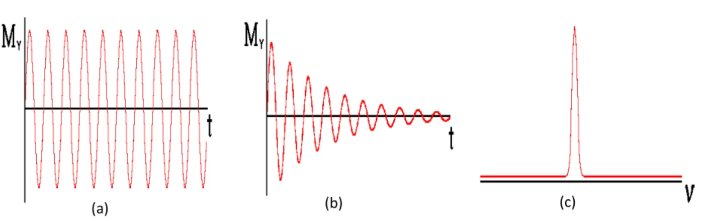
n-of B0. betwee follow axis an wire lo spins s time T conver Figur start signa Where - Mxyo is pulse c There are The comb en the T2 fr ws [6]: When a 90 nd this mot ocated aroun start to diph T2*. This d rted into a fr re 1-6:(a) A to diphase al [4] [6]. s the magni ceases). two factors bination of rom molecu 0° RF pulse tion will pro
nd of Ox ax hase with th ecay signal frequency do (a) After applic when the p tude of the s that affect f two factor lar processe ∗ is applied, oduce a sin xis (Figure he time T2* l is called omain spect cation of a 9 pulse turns
transverse m t on T2: the r above is t es and that f
M0 tips to X ne wave cur 1-6-b, Figur *. Therefore free induct trum by Fou 90° RF puls off. (b) Th magnetizatio molecular the time co from inhom XY plane (F rrent which re 1-7-a). W e, the corres tion decay urier transfo
lse, the prot e coil is pl on at t=0 (th interactions onstant calle mogeneity in Figure 1-6-a is a functio When the RF sponding w (FID) (Figu orm (figure I
ton spins tip laced on Ox he time at w s and the in ed T2*. The n the magne a). It rotates on of time i F pulse is tu wave will de ure 1-7-b). I.7-c). (b p to transve x axis to de (1-6 which the 90 nhomogeneit e relationshi etic field is a (1-7 about the O in the coil o urned off, th ecay with th The FID b) erse plane a etect the de 6) 0° ty ip as 7) Oz of he he is and ecay
1.3 Signal to noise ratio
The concept of signal to noise ratio (SNR) for NMR is first proposed by Ernst et al [7] in 1966 and applied to Micro-NMR by Odelblad [8] in the same year . The SNR is defined as the ratio of the amplitude of the signal to the average value of the noise. It is an important criteria to analyze the sensitivity of detection systems [9][10] in NMR experiments. Therefore, it is necessary to compute the SNR for evaluation of the quality of the detection of the NMR signal. This evaluation involves both ability of the system to detect the signal and the influence of the noise on this system.
1.3.1 The signal
There are numerous detection devices of NMR signal proposed by previous researchers. These devices have been used in the specific experimental conditions. The Superconducting Quantum Interference Device (SQUID) [11][12] and the mixed-sensor [13][14] is only operated in a low magnetic field condition. Another method is Cantilever (force detection) [15][16] which is suitable for the samples with nano size. The most popular device used to detect NMR signal is conductive coil due to the simple use and good intrinsic sensitivity. D. I. Hoult and R. E. Richards [9] proposed an approach to calculate the signal to noise ratio of the conductive coil using the principle of reciprocity. This method considers an arbitrary loop S where a unit current circulates and an arbitrary point P locates in the free space. The unit current creates a magnetic field B1 in the loop. They are placed in the static magnetic field B0 which is perpendicular to B1 as shown in Figure 1-8.
(a) (b) (c)
Figure 1-7: The current is plotted as a function of time and decay with the time T2* due to the
elemen potent located equatio F p Considerin ntary loop o tial of an ele Where: - r is the - The de The total f The eleme d at the poin We consid on (1-10) ca Thus the e Figure 1-8: induces on proportiona ng that the of unit curre ementary loo e distance fr erivatives ar field produc ent magneti nt P is:
der that the an be writte electromotiv (a) : The induc the loop S al to the B1 f surface S c ent. There ex op producin rom P to the re taken on t ced by the lo ic flux dF p
.
e dipole n as followive force (EM ction princip S an electr field at that consists of e xists a magn ng at the poi
.
e elementary the coordina oop is: passes throu.
is constant ing:.
.
MF) inducedple and sign romotive fo t point. elementary netic pseudo int P is: y loop ates of poin
.
ugh the elem
.
t through sp d in the loop nal receptio orce (EMF) loops of su o scalar pote nt P ment loop g pace and d p is given by (b) on [9][10]. ( . (b) The s rface dS bo ential at the generated by d is also c y:(a) The rota signal from ounded by a e point P. Th (1-8 (1-9 y a dipole (1-10 constant. Th (1-11 ation of Mxy m point P i an he 8)
9) 0) he 1) xy is
.
.
(1-12)We substitute the equation 1-9 to the equation 1-12. We have:
.
(1-13)This result is called the principle of reciprocity. The equation 1-13 was validated for the intermediate and radiation zone fields [17]. This equation is applied to calculate the signal induced by spins precession [9][10].
After the 90° pulse, the net magnetization M0 of the sample tips to transverse plane and rotate away from the longitudinal axis at an angular velocity (Figure 1-8) given by:
(1-14)
The rotation of the net magnetization M on the transverse plane produces an alternating magnetic field at the loop of conductor S (Figure 1-8-a). Using the principle of reciprocity, the EMF induced in the loop S is:
.
(1-15)Where:
- is the electromotive force induced in the loop S by elementary volume of
the sample.
- B1 is the magnetic field created by unit current i.
Thus the electromotive force EMF induced in the loop S by the volume V of sample is:
∭
.
(1-16)The behavior of the net magnetization M0 is described by the well-known Bloch equation [18][19]:
(1-17)
Where:
-
,
,
:
are the unit vectors in Ox, Oy and Oz directions of respectively.
- T1, T2 are the longitudinal and transversal relaxation time respectively.The magnetic field B1 produced by the sinusoidal current in the loop S is:
The NMR signal is only received on the transverse plane, thus the component is ignored. Hence the equation 1-18 can be written as:
(1-19)
Where:
-
is the unit vector of
.
- is the magnitude of
.
We substitute the equations 1-17 and 1-19 into the equation 1-16, then, we have:
∭
.
(1-20) And ∗(1‐21)
.
(1-22)
.
(1-23) Where:- M0 and ∗ are given by the equations 1-1 and 1-7 respectively.
Substitute the equations 1-21, 1-22 and 1-23 into the equation 1-20, the integral simplifies to:
∗
(1-24)
If the tip angle θ = 90° and B1 is homogeneous over the sample volume. The amplitude of NMR signal of a pulse RF is:
(1-25)
1.3.2 The noise
In NMR experiments, the noise of the detection systems mostly comes from the thermal noise associated to the resistance of the coil while other noises such as radiation, sample are negligible [20]. The thermal noise is given by formula:
∆
(1-26)Where:
- 1.38 ∗ 10 is Boltmann constant.
- Tp (K) is the temperature of the coil. - R is the electrical resistance of the coil. - ∆ is the detection bandwidth.
1.3.3 The sensitivity
The sensitivity of detection systems refer to the signal to noise ratio (SNR). It is defined as the ratio of the NMR signal (equation 1-25) to the noise (equation 1-26).
∆ (1-27)
√ (1-28) The equation 1-28 is used to evaluate the sensitivity of the antennas and optimize the configuration of antennas [21].
1.4 T1 and T2 measurements
1.4.1 T2 measurement
Both T1 and T2 are important in NMR experiment. However, the measurement of T2 relaxation is more practical because it can be obtained quicker than T1. There are two well-known techniques which are used to measure T2.
Firstly, Spin echoes or Hahn’s echo, this technique was first discovered by Hahn in 1950 [22]. The echo is a signal which has first vanished with time and then reappears some time later. The Hahn echo consists of two pulses, the first one is 90° pulse and then followed by 180° after the delay time τ as shown in Figure 1-9.
Figure decay; sequen Oy ax the tim inhom those second rotate into la period receive pulse, as CPM [24] an known 180° p two 18 measu e 1-9: Hahn ; τ is the de nce [22]. After the f is. Initially, me τ after w mogeneity of with lower d 180° pulse around Oz ag, in contra d of time τ, e coil. This T2 can be the amplitu Secondly, MG pulse s nd modified n Carr-Purc pulse which 80° pulse is ure the time
n echo with elay time be first pulse, t , the transve which the 9 f the static Larmor fre e is applied axis. Now t ast, the spins , all the spi phenomeno determined ude of transv the pulse s sequence. Th d by Meiboo ell-Meiboom h lead to the called the e e T2 (Figure h two pulse etween two
the net mag erse vector 90° pulse is field. Some equency lag along Oy a the phases o s with lower ins refocus. on is called d by measu verse magne sequence us he CPMG s om and Gill m-Gill (CPM formation echo time T e 1-10). Th sequence u pulse and T gnetization i M0 is a sin s turned off e nuclei wit g behind. A axis. All the of the spins r Larmor fre . Because t spin echo. uring the int
etization is d
sed to measu sequence wa l after four y MG) seque a train of ec E. The deca he amplitud used to mea TE is the in is transvers ngle vector b f, the nucle th higher La At a period spins are m s with highe equency tran the spins re terpolation defined by t
ure the tran as first intro years [25]. T nce. It cons choes after ay of the am de of the sp asure T2. FI nter-echo sp al to the XO because the ei are loss o armor frequ of time τ a mirrored aro er Larmor fr nsform lag efocus, they of the curv the equation nsverse relax oduced by C The resultin sist of one the delay ti mplitude of th pin echo is FID is the fr pacing used OY plane a e nuclei are of coherenc uency rotate after the fir ound OY and frequency tr into lead. T y generate a ve . Afte n (1-29) [23] xation time Carr and Pu ng sequence 90° pulse a ime τ. The t he spin echo weaker tha free inductio d in the puls nd lies alon in phase. A ce due to th e faster whi rst pulse, th d continue t ansform lea Thus, after th a signal in er the secon ]. (1-29 T2 is know urcell in 195 is now wel and series o time betwee oes is used t an the initi on se ng As he le he to ad he a nd 9) wn 54 ll-of en to al
amplit Fig toward saturat The si as a fu efficie the po pulse. describ grow b the ma be com tude by a fac gure 1-10: C produce 1.4.2 T1 The time T ds its equiril tion recover The satura ignal after e unction of co ent method f While the ositive Oz ax Immediate bed by the because ther agnetization mputed by e ctor of CPMG seque e a train of measurem T1 is decay lium value ( ry and the in ation recove each pulse is ontinuously for measurin inversion r xis to the n ly after the equation 1-re is no tran n into the pl equation 1-4 [26]. ence: After echoes. The ment constant fo (M0). There nversion rec ery uses a se s given by e y increasing ng T1.
recovery seq negative Oz e stimulus, -4. It can no nsverse com lane of the r 4. the initial 9 e NMR signa or the Z com e are two co covery [26]. eries of 90° equation 1-3 recovery tim quence initi axis as sho the spins st ot be direct mponent. Th receiving co 90° pulse, a al is detecte mponent of t mmon pulse ° pulses with 30 [26]. By me τ, the tim
ially uses th own in Figu tart to flip tly measure erefore, the oil where it series of 18 ed by the dec the longitud e sequence h the separa y recording t me T1 can b he 180° puls ure 1-11 an back at the d by the tim e subsequent t can be me 80° pulse is cay of T2[2 dinal magne used to mea ation τ to ca the echo sig be determine se to invert d then follo e rate of 1 me which th t 90° pulse asured. The applied to 7]. etization (M asure T1: Th ancel the M gnal intensit ed. This is a (1-30 the Mz from ows by a 90 , which he vector M is used to ti e time T1 ca Mz) he Mz. ty an 0) m 0° is Mz ilt an
Figur condit immob appear import the ec coeffic detail freque initial re 1-11: A s cor 1.4.3 Sel In NMR e tion for them bile and dif rs in the law tant in the c cho amplitu cient can be in [23]. The samp ency is then: Neglecting 90° pulse is M depend The equati sequence of rresponding lf-diffusion experiments m refocus a ffuse in spac w governing context of in ude, the va e obtained b ple is placed : g the effects s: s only on th ion 1-33 yie f experiment g FID is plot n and field g s, the spins after the sec ce. Their m the diffusio nhomogeneo alues of bo by observin d in a stron s of relaxati , he space com elds: in which th tted against gradient experience cond pulse. moving is ch on of the loc ous field. Th oth the tran ng the decay
ng field gr
ion and diff
mponent Z a
he recovery t the variabl a constant However, haracterized cal magnetiz hrough an a nsverse rela y of the ech adient fusion, the m
and the diffu
time are 0, le recovery steady field spins in the d by the diff zation m [2 analysis of t axation time hoes. This a in di magnetizatio usion equati t1, t2, t3 an time [26]. d. This is a e liquid sam fusion coeff 8]. Self-diff the effect of e T2 and t analysis can irection Oz, on at the tim ion is: d t4 and the an imperativ mples are no fficient whic fusion is ver f diffusion o the diffusio n be found i , the Larmo (1-31 me t after th (1-32 (1-33 e ve ot ch ry on on in or 1) he 2) 3)
(1-34)
and
(1-35)
The amplitude of the spin echo is weaker than the initial amplitude by a factor of
.
The echo amplitude at the time 2τ is:(1-36)
When using a pulse train and observing the various echoes, the amplitude of the nth echo at the time 2nτ is:
(1-37)
Or else, as a function of time 2 , the equation 1-37 can be written:
(1-38)
This is an exponential function of time, both D and T2 are possible to retrieve with the rate constant that depends on the interval 2τ between the pulses:
(1-39)
1.5 Influence of magnetic field homogeneity on NMR spectroscopy
The homogeneity of magnetic field is an important criteria which influents on the NMR signals. Therefore, it is necessary to emphasize the extremely homogeneous fields for NMR spectroscopy (MRS) when design a portable NMR device. NMR is the result of Zeeman Effect on the nucleus. The external part of the spin Hamiltonian which describes the interaction of the spins with magnetic environment is given by the equation 1-40 [18]:
,
(1-40)∑
(1-41)∑
(1-43)Where:
- is the interaction of each spin Ij with the external static field B0. - , is the interaction of each spin Ij with the gradient field Bgrad.
- is the interaction of each spin Ij with the RF field BRF generated by the RF coil. Some of these interactions are proportional to the external field (chemical shift), some are not (dipolar coupling), but always remain in the order of the part per million (ppm) of the main Zeeman Hamiltonian. The small changes of the static field B0 in each point of the sample will affect on the Larmor frequency. Hence, MRS requires sub-ppm over the volume of sample in
order to be useful [29], for example, ∆
10
across the sample for good spectroscopicresolution [30].
Chapter 2
Portable NMR system
Summary:
- Introduction- The need of portable NMR devices - Portable NMR devices
- The applications of NMR devices
- The components of portable NMR devices - Motivation for this work
Chapter 2: Portable NMR system design
2.1 Introduction
The field of portable NMR devices has been rapidly developed in the past few years. In the early time, the NMR devices are large, expensive and complicated devices. They are usually used in laboratory and are not portable. They use superconducting magnet to generate the field B0. Such devices generate the homogeneous field, consume too much energy and need high cost of maintenance.
The need of external applications of the laboratory motivates the development of portable NMR devices. There are varieties of portable NMR devices that have been done by previous researchers such as NMR-MOUSE, Mandhalas and well-logging etc... The shapes of the magnets depend on the end uses. For example, the Ex-situ devices are suitable for the samples with large size and placed outside the magnets while in-situ devices are suitable for the small samples and high resolution experiments due to high field strength and homogeneity are more easily achieved with such geometries. The portable NMR devices are used for many applications such as oil industry, medicine and materials….
The objective of this chapter is to introduce the development of portable NMR devices from the early time until now. In addition, we will present the different kinds of them and their diversity applications as state of the art.
2.2 The need of portable NMR devices
In 1952, one dimensional MRI image is reported by Herman Carr in his PhD thesis [1]. Much later on, in 1973, Paul Lauterbur and his team expanded the Carr’s technique and introduced the way using magnetic field gradients to obtain the images of objects in two dimensions and three dimensions [2]. The major drawback of NMR is its lack of sensitivity. This lack of sensitivity makes difficult the study of low γ nuclei in NMR spectroscopy by increasing the experiment time. The low sensitivity is also a limitation of MRI resolution [29]. One solution to solve this difficulty is to increase the external magnetic field in order to improve the SNR. Thus, the idea of the increase of magnetic field motivated many researchers performing experiments with high magnetic field.
Rabi and his team were performed the first experiment at a field of 0.6T (about 25.6 MHz) while Lauterbur’s experiment was done at a field 1.4T (60 MHz). In 1964, a superconducting magnet at 200 MHz was introduced by Nelson and Weaver [31] for the NMR spectroscopy
experi 23.5T The pr field B homog field a of doll they n limitat their w researc These NMR device source Figure [32]. ment. Since with the m rominent fea B0 more hom geneity, wei also have so lars). These need high co tion of high weight is als The develo chers to use magnets ca experiment es. Other at e of electric For these r e 2-1: The f e then, the machine insta ature of NM mogeneous
ight and dim ome disadva e machines a ost of maint h field NMR so a difficult opment of p e them for N an produce a tal requirem ttractive fea power and n reasons, the field homog field streng alled in the MR spectrosc than one w mension of antages. The are heavy an tenance and R spectrome ty for out of permanent m NMR applic a strong and ments. Thus, atures of pe no maintena e portable N geneity relat gth of NMR Centre de copy experi with low mag
magnets is e machine is nd have the consume m eters for wid f laboratory magnet tech cations, alth d homogeneo , this satisfi ermanent m ance. NMR devices
tes to the fie
R spectrome RMN “à tr iments with gnetic field. shown in t s very expen large dimen much energy dely applica application hnology such hough they ous field wh ied the cond magnets are s have been eld strength eters continu rès hauts ch high magne . The high f the Figure 2 nsive (some nsions. Bec y. Therefore ations of thi ns. h as rare-ea are applied hich is two i ditions for d obviously developed. h, weight an ues to incre hamps in Ly etic field is field associa 2-1. Howev e machines ause of larg e, these obst s technique arth magnets d for acceler important cr design of po the absence nd dimensio ease reachin yon, France the magnet ated the fiel
er, very hig cost million ge and heavy tacles are th e. In addition s has allowe rators earlie riteria for th ortable NM e of extern n of magne ng ”. ic ld gh ns y, he n, ed er. he MR al ets
2.3 applica sided, closed to show (region 2-2). T suitabl weight particu other a shaped Review of Normally, ations. The unilateral o d magnets or w the progr 2.3.1 Ex The ex-situ n of interest Thus, they c le for surfac t, they are d Ex-situ m ularly suited applications d, U-shaped f portable N the portabl first group w or ex-situ N r in-situ NM esses to be d x-situ porta u portable N t: ROI) near can use for t ce investiga difficult to a Figure 2-2 magnets der d to the cyli s have been d or a simple NMR devic le NMR dev with the me NMR. The MR. The exi done. ble NMR d NMR device r their surfa the experim ation. Altho achieve the h 2: The schem rive from indrical bor n tested. Th e bar magne es vices are di easured sam other group isting ideas devices es have the ace and the s mental objec
ough the ex-homogeneity matic of sing well-loggin eholes of oi he classical ets as Figure ivided into t mples placed p with the s of two grou simple conf samples are ct with unlim -situ magne y of magnet gle-sided or ng sensors il wells, sin geometries e 2-3. two groups d outside the samples insi ups will be figuration w e putted outs mited dimen ets have the tic field in th r ex-situ mag s. Apart fr ngle-sided se s of ex-situ due to the e magnet is c
ide the mag exposed bri
with the sens side the mag nsions. Such e simple sha he sensitive gnets. rom sensor ensors suite magnets ar objectives o called single gnet is calle iefly in orde sitive volum gnets (Figur h systems ar ape and ligh e volume. r geometrie ed for divers re usually C of e-ed er me re re ht es se