Classical and Semiclassical Studies of the Hydrogen Molecule

HAL Id: tel-02371554

https://tel.archives-ouvertes.fr/tel-02371554

HAL is a multi-disciplinary open access

archive for the deposit and dissemination of sci-entific research documents, whether they are pub-lished or not. The documents may come from teaching and research institutions in France or abroad, or from public or private research centers.

L’archive ouverte pluridisciplinaire HAL, est destinée au dépôt et à la diffusion de documents scientifiques de niveau recherche, publiés ou non, émanant des établissements d’enseignement et de recherche français ou étrangers, des laboratoires publics ou privés.

Molecule

Thomas Sauvaget

To cite this version:

Thomas Sauvaget. Classical and Semiclassical Studies of the Hydrogen Molecule. Chaotic Dynamics [nlin.CD]. University of Nottingham (UK), 2006. English. �tel-02371554�

Classical and Semiclassical Studies

of the Hydrogen Molecule

by Thomas Sauvaget

Thesis submitted to the University of Nottingham

for the degree of Doctor of Philosophy

The aim of this work is to account for the global shape of some Born-Oppenheimer (BO) curves of the hydrogen molecule, in particular the ground state, at the semi-classical level.

In the first two chapters we review semiclassical cycle expansion techniques which proved useful in the study of the resonant spectrum of the helium atom, another few-body Coulomb system.

Then we first study in detail the geometry of the classical phase space of the hydrogen molecule. This being done, we analyze the dynamics in three of its subspaces and compute various quantities related to their shortest periodic orbits.

We then turn to semiclassical studies. One of these subspaces is discarded on instability grounds, while the other two are used as a basis for the construction of semiclassical approximations to the ground state BO curve. We find that each of the two subspaces allow to describe one of the two asymptotic trends of the BO curve.

This allows to provide a classical underpinning to bond formation in H2.

First I would like to express my gratitude to my advisor Gregor Tanner. He patiently taught me a lot about physics and was always willing to discuss things out. I would also like to thank him and his family for being so kind with me in Bristol and Nottingham.

Next I would like to thank Stephen C. Creagh for several very useful discussions in the past years, in particular during the first year when Gregor was in Bristol.

From Leicester I thank very much Ben Leimkuhler, whose enthousiastic semi-nars have broaden a lot my knowledge of numerical simulations. Thank you also to Chris C. Sweet and Ruslan Davidchack for showing me some of their C++ codes, where I first learnt about several libraries and tricks.

My research was made possible by funding from the EC network MASIE super-vised by Mark Roberts. I would like to thank him, and all those I have met during our many conferences, for such a stimulating atmosphere.

The Baines family has been very kind to me in many ways and I would like to thank them very much for their invitations and help.

On the french side, Marc Legrand’s enthousiasm and discussion-style lectures have had a great impact on the second half of my undergraduate curriculum, and on my thinking more generally; I am grateful for that influence.

Finally I would like to express my most profound gratitude to my dear pa-rents, my fantastic brother, and all my beloved family for their continuing love and encouragements.

This work is dedicated to: My Parents

&

Mr Douglas Whitelaw FRCSEd FRCS, General Surgeon; Mrs Kontouli, Anes-thesist; the theatre crew; the nurses of the High Dependency Unit; the nurses and staff of the Cobham clinic; the physios; and the ambulance crew of the Luton and Dunstable Hospital.

“[...] the status of the continuum hypothesis convinced me that Platonist views of mathematical ontology and truth could not be correct [...]”

Abstract . . . i

Acknowledgements . . . ii

List of Figures . . . viii

1 Introduction 1 1.1 Approximations in quantum mechanics . . . 2

1.1.1 Basic setup . . . 2

1.1.2 Exact solutions . . . 3

1.1.3 Direct numerical solutions . . . 5

1.1.4 Approximate asymptotic eigenfunctions . . . 7

1.2 The semiclassical limit of quantum mechanics . . . 8

1.2.1 Setting . . . 9

1.2.2 Case of an integrable limit . . . 10

1.2.3 Case of an hyperbolic limit . . . 19

1.3 Organization of the thesis . . . 32

2 Few-body Coulomb problems 34 2.1 Motivation . . . 34

2.2 Hydrogen molecular ion . . . 35

2.2.1 Setting . . . 35

2.2.2 Solution of the quantum problem . . . 36

2.2.4 Semiclassical limit: tunneling geometry, monodromy and

bi-furcations . . . 41

2.2.5 Adiabatic invariant and dynamics beyond the BOA . . . 45

2.3 Helium atom: experiments and quantum aspects . . . 47

2.3.1 Experimental imput and spectral structure . . . 47

2.3.2 Quantum approaches . . . 49

2.4 Helium atom: semiclassical aspects . . . 54

2.4.1 Setting . . . 54

2.4.2 Scaling property . . . 56

2.4.3 Collision singularities . . . 56

2.4.4 Symmetries, integrals and reduced space . . . 63

2.4.5 Collinear eZe dynamics . . . 68

2.4.6 Collinear Zee dynamics . . . 72

2.4.7 Planar dynamics . . . 72 2.4.8 Semiclassical quantization . . . 76 2.5 Hydrogen molecule . . . 79 2.5.1 Quantum aspects . . . 79 2.5.2 Semiclassical approches . . . 81 2.6 Numerical methods . . . 83

3 Classical dynamics of the hydrogen molecule 85 3.1 Introduction . . . 85

3.2 Setting . . . 86

3.3 Scaling property . . . 88

3.4 Collision set . . . 89

3.5 Symmetries, integrals and reduction . . . 89

3.5.1 Continuous symmetries . . . 89

3.5.2 Discrete symmetries . . . 91

3.6.1 Dynamics of the eZZe configuration . . . 93 3.7 Dynamics in N{e} . . . 108 3.7.1 Setting . . . 108 3.7.2 Flow . . . 110 3.7.3 Fixed points . . . 112 3.7.4 Invariant subspaces . . . 112

3.7.5 Dynamics in the collinear pendulum configuration . . . 124

3.7.6 Dynamics in the Z⊥ configuration . . . 130

4 Semiclassical quantization of the hydrogen molecule 140 4.1 Quantization of the eZZe configuration . . . 140

4.2 Quantization of the Z⊥ configuration . . . 143

4.3 Bond formation mechanism . . . 145

5 Conclusions 147 5.1 Symmary of results . . . 147

5.2 Future work . . . 148

A Notations for classical mechanics 149 B Group theory and the hydrogen atom 155 B.1 Geometrical group . . . 155

B.2 Degeneracy group . . . 157

C Reduction theory for Hamiltonian systems 161 C.1 Setting . . . 161

C.1.1 Symmetry group and integrals . . . 162

C.1.2 Isotropy types and invariant manifolds . . . 163

C.1.3 Free and non-free actions . . . 164

C.1.4 Energy momentum map . . . 165

C.3 Singular reduction . . . 167

1.1 Some potentialV when N = 1 . . . 10

1.2 The momentum is a multivalued function of the position . . . 11

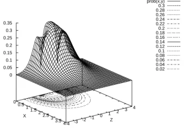
2.1 Probability density of ground state ofH₂+ (part 1) . . . 38

2.2 Probability density of ground state ofH₂+ (part 2) . . . 39

2.3 Probability density of ground state ofH₂+ (part 3) . . . 40

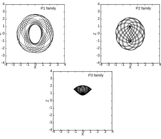
2.4 The three periodic orbit families ofH₂+ atLz = 0 . . . 42

2.5 EBK and uniform EBK results for low-lyingH2+states . . . 43

2.6 Zhilinski´ı diagram of monodromy inH₂+ . . . 45

2.7 The numerical spectrum of1_Se _{helium states . . . . 48}

2.8 Helium eZe and Zee collinear configurations . . . 66

2.9 Planar helium configuration . . . 67

2.10 Contour plot of energetically allowed configuration space domain . 67 2.11 Typical orbit of eZe . . . 69

2.12 Poincar´e section of eZe . . . 69

2.13 Short orbits of the eZe configuration . . . 71

2.14 One GS orbit in physical, reduced, and MO coordinates . . . 74

2.15 Triple collision manifold of eZe . . . 75

2.16 Conveyor belt mechanism between triple collision and double es-cape points . . . 75

2.17 Numerical results of semiclassical cycle expansion of eZe . . . 78

2.18 Potential energy curves of lowest1_Σ+ g electronic states ofH2 . . . . 80

3.1 Classical hydrogen molecule . . . 87

3.2 Four collinear hydrogen configurations . . . 91

3.3 Poincar´e sections of eZZe (part 1) . . . 96

3.4 Poincar´e sections of eZZe (part 2) . . . 97

3.5 Evolution of eZZe initial conditions on the PSOS . . . 100

3.6 R-dependence of the period and action of an eZZe orbit . . . 100

3.7 Types of linear perturbations of eZZe . . . 103

3.8 R-dependence of Lyapunov and stability exponents of an eZZe orbit 105 3.9 Effect of parametric triple collision on linear perturbations of eZZe 106 3.10 Gel’fand-Lidskii index of the_{R − 1 orbit at R=3 . . . 107}

3.11 Equilibrium of the hydogen molecule . . . 113

3.12 The Z (4 DOF) and Z_⊥(3 DOF) subspaces . . . 114

3.13 The 2 DOF configurations Wρ and Wz . . . 116

3.14 The 2 DOF configurations S and P . . . 117

3.15 The 2 DOF configuration Wρ,⊥ . . . 118

3.16 Organization of the various invariant subspaces . . . 119

3.17 Contour plots of P . . . 120 3.18 Contour plots of Wρ,⊥ . . . 121 3.19 Contours plots of Z⊥ . . . 121 3.20 Contour plots of Wρ . . . 122 3.21 Contour plots of S . . . 122 3.22 Contour plots of Wz . . . 123

3.23 Poincar´e sections of P (part 1) . . . 126

3.24 Poincar´e sections of P (part 2) . . . 127

3.25 Asymmetric nonlinear normal mode of P . . . 127

3.26 Pair of orbits created at the first saddle-node bifurcation . . . 128

3.27 Asymmetric nonlinear normal mode vs pseudo-asymmetric-stretch orbit . . . 129

3.29 Continuation of eZe orbits in Z⊥(part 1) . . . 133

3.30 Continuation of eZe orbits in Z⊥(part 2) . . . 134

3.31 Continuation of eZe orbits in Z⊥(case of RPO) . . . 135

3.32 Schematic description of the non-smooth limit of momenta at the origin . . . 135

3.33 Orbit whose limit is forbidden by grammar rules . . . 136

3.34 R-dependence oc action of an R-eZe orbit . . . 137

3.35 Stability exponents of the_{R − 1 orbit . . . 138}

3.36 Stability exponents of the_{R − 01 orbit . . . 139}

4.1 Semiclassical approximation built on the eZZe asymmetric stretch orbit (electronic energy) . . . 141

4.2 Semiclassical approximation built on the eZZe asymmetric stretch orbit (total energy) . . . 142

4.3 Semiclassical approximation built on the_{R − 1 orbit of Z}⊥(small R range, electronic energy) . . . 143

4.4 Semiclassical approximations using only the actions of the Z⊥ PO, this up to code length 1, 2, and 3. . . 144

4.5 Combination of eZZe and Z⊥ semiclassical approximations (elec-tronic energy) . . . 145

4.6 Combination of eZZe and Z⊥semiclassical approximations (total en-ergy) . . . 146

C.1 Regular reduction . . . 166

Introduction

Since the advent of quantum mechanics (QM) at the beginning of the XXth century, it has been possible to predict and organize a lot of phenomena involving atoms and molecules (see e.g. [BJ03, BC03, SO96]).

There are nevertheless various aspects requiring calculations which are very intensive and time-consuming, and sometimes in fact intractable. In those cases it is thus useful to develop approximations of QM which, while being possibly less acurate, still provide enough information to obtain similar predictions and understanding but at a much reduced cost (see §1.1).

An important related topic is to understand how quantum mechanics leads to behaviours well described by classical mechanics, and more generally to study how the formalisms of these two theories are related (see §1.2).

The aim of this thesis is to address a particular problem which lies at the inter-section of these two thematics, namely to describe the structure of some electronic states of the hydrogen molecule by using the so-called semiclassical approximation

1.1

Approximations in quantum mechanics

The aim of this chapter is to describe in some detail what is called the semiclassical

limit of quantum mechanics, and the kind of approximation it allows in various

sit-uations. To put it into proper context we first review other exact and approximate methods used over the past decades in quantum mechanics, stressing their domain of applicability.

1.1.1

Basic setup

Suppose we are studying a simple quantum system, i.e. one which can be modelled as taking place in a finite-dimensional flat configuration space RN_{, and which is}

also time-independent and of the form ‘kinetic plus potential’. N is the number of

degrees of freedom (DOF). The main example is that of a general _{n−body system}1

in constant external fields. We suppose moreover that relativistic and spin effects can be neglected.

We are therefore led to study the usual eigenvalue problem for the corresponding (linear) Schr¨odinger operator bH:

b Hψk := N X i=1 − ~ 2 2mi ∆iψk+ V ψk = Ekψk (1.1)

whereEk is real and the wavefunctionψk ∈ L2(RN) is decaying to 0 at infinity.

Of course in all the following we will assume that nothing pathological happens, but without making very precise statements. For example we are assuming that V is such that bH is self-adjoint on some domain – and has thus indeed a real spectrum – and is bounded from below. This is for example the case if V is a Kato potential [HS00], i.e. if for any positive real numberα and all smooth ψ which decays to 0 at infinity we can find a number_{β = β(α) such that V satisfies the bound kV ψk ≤}

1

Here n is the number of bodies, so for example in the case of bodies moving in 3−dimensional space we would have N = 3n.

α kT ψk + β kψk, where T is the kinetic energy operator. In particular, n−body

Coulomb potentials, on which we will focus in chapter 2, are Kato potentials.

Other quantites of interest after the discrete (real) eigenvalues are discrete (complex) resonances Fm = Em − iΓm ∈ C. They exist when some of the

coor-dinates of our configuration space can go to infinity (scattering process). There are various possible definitions depending on the form of V (e.g. wether it is long-range or short-long-range [Zwo99]), but roughly speaking resonances are isolated com-plex poles of some meromorphic continuation of the resolvent( b_{H − s b}I)−1_{, the real}

poles being the eigenvalues (the parameter s being real). In the time-dependent Schr¨odinger equation, a time-dependent damping factor thus comes in and the decay rate of such states is given by the imaginary partΓm of the resonance.

Let us see now how to actually compute at least some eigenvalues and reso-nances of our _{N −dimensional Hamiltonian, possibly together with the} eigenfunc-tions.

1.1.2

Exact solutions

The first idea coming to mind is of course to look for exact solutions, but we must be slightly more precise. Indeed we could ask, from more general to more specific, for

(a) exact but not necessarily explicit solutions; (b) explicit solutions given by (convergent) series;

(c) explicit solutions given by a single non-elementary function; (d) explicit solutions given by an elementary function. 2

The literature is a bit confusing on this topic since there are authors who reserve the usage of the word exactly-solvable for either of those cases.

2_{i.e. not involving special functions. Recall that a theorem by Liouville, generalized by Ostrowski} and later Rosenlich [Ros72], says that not all elementary functions have elementary antiderivatives, for example F :=R sin(x)_x is not an elementary function.

Case (a) covers for example the situation where (say) the first m eigenvalues (or all of them if the spectrum is finite) are recast into being unknown solutions of a nonlinear system of equations which is itself known explicitely. This is the case in the work of Voros [Vor05] on the 1D polynomial Schr¨odinger equation of any degree (where in fact in this case the full infinite spectrum is characterized). In many other areas of physics where one studies Hamiltonians not of the form (1.1), for example second-quantized operators in nuclear or condensed matter physics [DPS04], one also calls these problems exactly-solvable in such a situation.

On top of that, either our Schr¨odinger PDE is separable into a setN uncoupled ODEs by a suitable choice of coordinates or it is not. In both cases one then may, or may not, find the spectrum and eigenfunctions explicitely. Of course this is much simpler in the separable case, where examples have been known for a long time in all four situations (a-d).

In the 1D case, it has recently been shown [BG03] that several widely used model potentials including:

VHO(x) :=

ω2_x2

2 (harmonic oscillator potential) (1.2) VM(x) := B2e−2αx− B(2A + α)e−αx (Morse potential) (1.3)

VRC(x) := −

e2

x +

ℓ(ℓ + 1)

x2 (rotational-Coulomb potential) (1.4)

all belong to an explicitely known family of potentials (depending on eight param-eters and a level-dependent scalar) which are solvable in the strongest possible sense, namely (d).

On the other hand examples of non-separable_{N −dimensional potentials whose} spectrum and eigenfunctions are known in the sense of (c) were apparently found only a few years ago [BEE+_{02]. These are periodic potentials related to models of}

fair amount of complex analysis.

But it remains that many systems of great interest are not solvable in any of the above senses – in particular, the_{n−body Coulomb problem of atomic and} molec-ular physics is not – and therefore one is led to find methods of approximations which work for any potential.

1.1.3

Direct numerical solutions

The most natural potential-independent approximation one could think of is simply to solve the eigenvalue problem (1.1) numerically at some prescribed order of accuracy. In computational chemistry this is called an ab initio method. Again there are many ways to do this.

From the traditionnal point of view of numerical analysis, one would consider (adaptive) mesh-based methods like finite differences and finite elements (FEM), but these do not have favorable scaling properties with respect to the dimensionN of the system. The corresponding literature is thus rather scarce, including in the Coulomb case [ZY04].

Much more successful methods are those based on the variational formula-tion of the problem, namely (1.1) is seen as an Euler-Lagrange equaformula-tion (the sta-tionary solution we are looking for being a minimum). The key step is then to find a suitable orthogonal basis (ϕk)∞k=1 of the (huge) variational space H1(RN).

Indeed, in this direct route one wishes to use trial wavefunctions of the form ψd(x1, . . . , xN) =Pk=1d ckϕk(x1, . . . , xN). The best set of coefficients, in the case of

the ground state, then corresponds to the global minimum of the _{d−dimensional}

Rayleigh-Ritz ratio

ERR(c1, . . . , cd) = hψd| bH|ψdi

hψd|ψdi

For higher states the minimization must be done under the constraints of or-thogonality with the lower states. Thus the basis should allow a fast evaluation of the matrix elements (integrals on two copies of the configuration space) while requiring a low number d of members (at the level of chemical accurary) to be of any use. In practise, at least in the Coulomb case of atoms and molecules, finding such a basis is not possible even for systems of relatively small size (say, N = 30) [LBge03].

For larger systems one therefore seeks further approximations by restricting the variational space. For example, in atomic physics the Hartree-Fock approximation assumes that the Hamiltonian can be split into n weakly interacting parts (indi-vidual electrons terms) whose interactions are neglected except from a common averaged one. Using those one-electron orbitals φi, the variational wavefunction

then has the form of a Hartree productψd =Qn_i=1φi (or is an antisymmetric Slater

determinantdet(φi) if one wishes to take into account the Pauli principle). So only

a good basis of the smaller space H1_(RN

n) is needed. The solution is then found

iteratively (due to the self-consistency constraint of the averaged electronic interac-tion) by solving a generalized eigenvalue problem associated to the Fock matrix, rather than minimizing the energy as in the direct method. Interactions can then be taken into account by using sums of determinants rather than a single one (configuration-interaction (CI) method). See [Pop99, SO96, LBge03] for a detailed introduction to such wavefunction-based methods. In particular, the rate of con-vergence of the expansion remains the most fundamental issue, see also [Kut05]. Other methods to account for correlations include the coupled-clusters one, which can be very powerful [NE05].

Yet, for even larger systems the approximately constant number P of new or-bital parameters needed per added degree of freedom implies the existence of an

exponential barrier PN _{[Koh99], and one thus needs yet another form of}

coworkers realized that the electronic densityρ – which lives in H1_(R3_{) – contains}

exactly the same information as the full wavefunction provided one uses a certain (unknown) functional. The impact of this Density Functional Theory (DFT) has been tremendous in the analysis of large systems, despite the use of only approxi-mate functionals. For a more mathematically oriented approach to these and other related issues one should refer to [LBL05, KM05].

These numerical approximations are mainly aimed at computing low-lying states and in particular the ground state, the high-lying ones being out of reach except for small enough systems.

Finally, calculations of resonances (see [BC71], [Moi98] and [Lin02]) are usu-ally done by performing a complex scaling3 _{of the space variables. One then looks}

at the real spectrum of a corresponding scaled non-self-adjoint complex operator, either analytically or numerically.

1.1.4

Approximate asymptotic eigenfunctions

Matched asympotic expansions are used as a method of approximation in many areas of applied mathematics. Let us take again the example of _{n−body Coulomb} problems, where its use is in fact quite recent so that only some few-body systems have been considered so far.

In a series of papers [KPTT96, PTT99, Pat99, Pat00, Pat03], Patil and coworkers have used the constraints on the exact wavefunction coming from collisions of pairs of bodies (like the famous Kato cusp condition at electron-nucleus collision) and from escape at infinity. There is a prescribed behaviour in these regions, and some global approximate wavefunctions are found by matching those local expressions under some assumptions on electronic interactions and overall symmetry. We shall

3_{In the mathematical literature when such scaling is valid one says that the Hamiltonian has} the dilation analycity property.

consider these results in more details when discussing the helium atom in chapter 2.

Since the consideration of the numerical precision of the approximate eigen-value alone is not a very sensitive test on the quality of the corresponding approx-imate eigenfunction (this is the quasi-mode problem, see appendix 11 in [Arn89]), one uses the so-called local energy test. This simply means that an approximate wavefunction eψ of good quality must be such that the ratio of the values of the two functions bH eψ and E eψ is very close to 1 and slowly varying over the whole config-uration space. It is indeed the case for the wavefunctions of Patil and coworkers.

The main issue to be surmounted in order to use this method on bigger atoms is, not surprinsingly, to find explicitly some approximate but accurate multi-electron interaction terms, which is not obvious.

1.2

The semiclassical limit of quantum mechanics

We shall now consider in some details another kind of useful approximation; it has two main related goals: (1) to provide reliable results for the high-lying states at a reasonable cost, (2) to understand the transition from quantum to classical mechanics.

It has been developed by the three different communities of mathematicians, physicists and chemists, each with its own motivations and emphasis. It is thus a very large subject and we shall only present it in the restricted framework of our eigenvalue problem (1.1) without stuying the various other situtations where similar methods have been developed (recent reviews describe in particular the cases of billiard-type systems [Wir99], field theories [MG03] and quantum graphs [GS06]).

There are essentially two textbooks which taken together cover most of the material we are interested in: the enjoyable online book [CAM+_{05] (in its latest}

and now quite complete version 11.0), and the textbook [BB] which is shorter and contains some complementary topics and various examples. An overview of some early developements in this area can be found in [Gut90]. We are going to sum-marize the relevant theoretical ideas, and leave calculations in concrete examples from atomic physics to the next chapter. See appendix A for some background on classical mechanics; we mark any first occurence of terms defined there with the symbol•_.

1.2.1

Setting

Our aim is to consider the formal and singular 4 _{limit ~ → 0 (which must recover}

classical mechanics as the commutation relations imply) and to find methods to compute the eigenvalues, and possibly the eigenfunctions, up to O(~2_{), at least}

in the cases where classical dynamics is fairly well understood (integrable•_{, and}

hyperbolic• _systems).

Other approaches relating classical and quantum mechanics have been devel-oped, but we shall not study them. In particular, we are not interested in construct-ing quantum systems from classical ones as in geometric quantization (see [Got99] for a precise statement of the Gr¨uwald-van Hove ‘no-go’ theorem which shows the limits of this approach). We are also not going to talk about the relations between the semi-classical limit and the ideas coming from deformation

quantiza-tion [DS02, CGSL+_{05b, CGSL05a].}

4_{i.e. the small parameter ~ is a factor of the highest order differential term of the Hamiltonian,} namely the Laplacian, hence at ~ = 0 there is a sudden drop of order.

1.2.2

Case of an integrable limit

Suppose that our classical limit is an integrable system with N DOF. Then there exists a well-known method, developped by Einstein, Brillouin and Keller (EBK

quantization5), which allows to locally construct in a neighborhood of a regular value f = (E, f2, . . . , fN) of the energy-momentum map• a lattice of approximate

quantum states together with their associated eigenfunctions. Let us first deal with the original construction (we make here a synthesis of Keller’s review [Kel85], some parts of Guillemin & Sternberg’s book [GS77], Murayama’s lecture notes [Mur04], and [Gut90,CAM+_{05]) and then we shall consider an alternative version}

with a more quantum flavor due to Littlejohn [Lit86b, Lit86a].

WKB method

Let us consider the case N = 1 succintly to notice the change of point of view offered by the geometric reformulation of the older WKB method, which itself goes as follows. Suppose

H(x, p) = p

2

2 + V (x) (1.6) with_{V satisfying V (x) ≈ x}2 _{nearx = 0 and lim}

|x|→+∞V (x) = +∞ x2 x1 E V (x) x III I _II

Figure 1.1: Some potential V when N = 1

5_{Sometimes also called torus quantization for obvious reasons. In the mathematical literature} the terminology Bohr-Sommerfeld quantization (which in physics refers to the narrower ad hoc method of action quantization of the “old quantum theory” of Bohr) is employed.

At a given energy E, configuration space splits into three regions: I and III are classically forbidden whileII is allowed, the boundaries between these regions being the two turning pointsx1 andx2 where the momentum vanishes. In fact the

momentum is a multivalued functionp = P (x) of the position since only the square ofp appears in H. The corresponding plot is

x1 x2 x

p

Figure 1.2: The momentum is a multivalued function of the position We now solve Schr¨odinger’s equation order by order in ~ with the ansatz

ψ(x) = A(x)e~iB(x) (1.7)

at a regular pointx.

At O(~0_{) we find 0 = (B}′₎2_{+ V − E. This is the Hamilton-Jacobi equation for}

B, the solution is hence the action B(x) = S(x) =

Z x x0

P (u)du + S0 (1.8)

where x0 is a reference point. S is then also a multivalued function since we must

pick a branch of P . These two branches simply have opposite signs and we can choose the conventionP2(x) = −P1(x) > 0.

At O(~1_{) we find}

0 = 2A′B′+ AB′′ = (A

2₎′_B′_{+ A}2_B′′

so we must have(A2_B′₎′ _{= 0: this is the continuity equation for a “quantum fluid”}

of densityA2 _{and momentaB}′_{. The solution is}

A(x) = p κ |S′_(x)| =

κ p

|P (x)| (1.10) for some constantκ.

Terms of higher order can be found recursively from here and are neglected. We hence end up with two (so-called Liouville-Green) local solutions

χk(x) =

κk

p

|Pk(x)|

e~iSk(x) (1.11)

corresponding to each branch Pk of P (and hence of S), and by linearity of

Schr¨odinger’s equation we get our local approximate solution as

φII(x) = χ1(x) + χ2(x) (1.12)

withκ1 and κ2 still to be determined. Similarly

φI(x) = α p |P (x)|e −1 ~ Rx x1|P (u)|du (1.13) and φIII(x) = β p |P (x)|e −1 ~ Rx x2|P (u)|du (1.14)

These local Liouville-Green solutions blow up at the turning points since Pj(xi) = 0, so in order to construct a global wavefunction we need to match the

local ones using the asymptotic properties of the exact wavefunction at x1 and x2.

This is done by using a linear approximation ofV near each xi, the exact solution

of the corresponding Schr¨odinger equations being the first Airy function Ai(s) = 1 π Z ∞ 0 cos(t 3 3 + st)dt (1.15)

whose asymptotic form at large_{|s| is known. It is then found that in the region II} the wavefunction should be at the same time of the form

C p P2(x) cos¡ Z x x1 P2(u)du − π 4 ¢ (1.16) and ±p C P2(x) cos¡ Z x x2 P2(u)du + π 4 ¢ (1.17) whereC is some constant. This is equivalent to the quantization condition

Z x2 x1

P2(u)du = (r + 2 ·

1

4)π~ (1.18) (with _{r ∈ N), an implicit equation in E (from the start E was a parameter in} Pj(x)) which singles out the discrete values Er at which such global approximate

wavefunctions exist. There are now definite relations between the coefficients of the three regions

C = β = κ1ei π

4 = κ₂e−i π

4 = (−1)rα (1.19)

EBK quantization `a la Keller-Maslov

In order to find analogous conditions in the general case N > 1 Keller and Maslov introduced a crucial modification of the geometrically invariant reformulation of the ad hoc Bohr-Sommerfeld rules that Einstein had presented earlier. Multiply-ing by 2 the WKB quantization condition (1.18) and using the fact that the two branches of P (fig. 1.1) can also be seen as forming a smooth submanifold of phase space, namely a_{1−torus T}E, we can rewrite the condition as

I

T_EP (u)du = (r + 2 ·

1

4) 2π~ (1.20) This is reminiscent of Einstein’s ad hoc action quantization condition except for the extra half-integer: a phase loss of π

points when going from one branch of P to the other, i.e. when comparing χ1

with respect toχ2. This last observation can be explained by using the method of

stationary phase to transform smoothlyχ1 intoχ2. In its general formulation6 this

states that from two functions a(u, v) and b(u, v) and a small parameter ǫ we can construct a function of the variablesu only by considering the oscillatory integral

ϕ(u) = Z

V

a(u, v)eiǫb(u,v)dv (1.21)

Its asympotic expansion in powers ofǫ at any given value of u is

ϕ(u) ∼ (2πǫ)d2 µX v∗ j eiπ4sja(u, v ∗ j)e i ǫb(u,v ∗ j) q |detG(u, v∗ j)| ¶ + O(ǫd2+1) (1.22)

where_{d is the dimension of the v−space, the v}∗

j are the points where the derivatives

∇vb vanish (we assume there is a finite number of those points), G is the Hessian

matrix of b with repect to the v variables, and sj is the signature of G at (u, vj∗),

which is what controls the additional relative phases. In ourN = 1 case, if we set ǫ = ~ and define

a2(x, p)e i ~b2(u,v) := e− i ~xpχ 2(x) (1.23) i.e. a2(x, p) := √κ2 |P2(x)|

and b2(x, p) := S2(x) − xp, then doing a stationary phase

with respect to p, propagating smoothly until reaching the P1 branch and going

back to _{q−representation (see [CAM}+_{05]) we find that indeed a phase loss of} π 2

has been introduced so that κ2 = κ1e−i π

2, i.e. κ₁ei π

4 = κ₂e−i π

4 just like the WKB

method showed.

In the case N > 1 the situation is now the following: we consider a regu-lar value _{f of the energy-momentum map of our integrable N −dofs Hamiltonian}

6_{The method of stationary phase is described in details in the very informative first chapter} of [GS77]. The rest of that old book, which covers also EBK quantization and other topics like geometric quantization, is written from a pure-mathematician’s point of view with very tedious general constructions and no attention to practical computational issues.

system and make the simplifying assumption that the fiber• _{is compact and}

con-nected: we have one torus Tf in phase space. This torus provides a cover of some

partW := ΠQ(Tf) of configuration space, where ΠQ is the projection onQ. Then

W can be decomposed into a union of disjoint open sets W = ∪jWj such that the

number NWj of pieces of Tf over any point q ∈ Wj is constant over the whole of

Wj, this for eachj. The common boundaries between the Wj, where the projection

is singular, is the caustic (set), analogous to the turning points of the N = 1 case. The existence of this covering shows that the momentap are multivalued functions of the positionsq.

The problem we face is then to match these local solutions at the caustics (where again the amplitudes diverge) to get a global solution. We thus have to compare each localχj term to the others through the caustics, and this is done by

considering each independent loop of a homotopy basis• _{C

k}Nk=1 of Tf. So we get

N implicit quantization conditions for f as I

C_k

P (q) dq = (rk+ µk·

1

4) 2π~ (1.24) where µk is an even integer called the Keller-Maslov index (of the loop Ck on the

Lagrangian manifold Tf with respect to ΠQ) which counts the number of times a

change of branch happens along Ck. The reason why we need only theseN

homo-topy conditions is that the action is an homohomo-topy invariant. This is easily shown by using the action-angle variables and Stokes’ theorem: pick two homotopic loops C and ˜Con Tf. Then Z C−˜C P dq = Z A∇ ∧ P dq = Z B∇ ∧ I dθ = 0 (1.25) since theI are constant.

EBK rules via wavepackets methods

There exists another method in the literature to derive the EBK rules which is due to Littlejohn. The idea is to work with the linear flows obtained by using the actions

Ik= 1 2π I C_k P (u)du (1.26)

as Hamiltonians. One can construct a semiclassical approximation of the associated quantum propagator

Vk(τ ) = e− i

~τ ˆIk (1.27)

using the metaplectic representation of the linearized dynamics around the trajec-tories of the flow ofIk, defined as follows.

Recall that there exists a 2-to-1 unitary representation of the symplectic group Sp(2N, R) by a group M p(2N, R) of operators acting on Hilbert space, called the metaplectic representation [GS84]. To any symplectic matrix S = ¡A B

C D

¢ there corresponds two operators (differering by a sign) given by

ˆ MSψ(x) = ±e−in π 4p 1 | det B| 1 (√2π)n Z RN eiW (x,y)ψ(y)dy (1.28) with W (x, y) = 1 2(DB −1 x · x + B−1Ay · y − 2B−Ty · x) (1.29)

Littlejohn then shows that Vkcan be approximated semiclassically by

V_ksc(τ ; z0) = e i

~(α(τ )−τ Ik(z0))_{T (z(τ )) ˆ}ˆ _M

S(τ )Tˆ†(z0) (1.30)

wherez(τ ) = (q(τ ), p(τ )) is a trajectory of the flow of Ik andz0an initial condition,

where α(τ ) := 1 2 Z z(τ ) z0 (pdq − qdp) (1.31)

is a symmetrized Bohr-Sommerfeld phase, and where ˆ

T (z) := e~i(pˆq−q ˆp) (1.32)

are Weyl-Heisenberg operators (which produce phase space translations).

Since_{S(τ ) is itself 2π−periodic around a 2π−periodic orbit of the flow of I}k, it

is found that

ˆ

MS(τ +2π) = e−iµk π

2Mˆ_{S(τ )} (1.33)

withµk thek−th Keller-Maslov index, and α(τ + 2π) = α(τ) + 2πIk(z0). So Ik(z0)

is an eigenvalue of ˆIkonly if its associated eigenstate exists, i.e. only if the Fourier

transform does not vanish |rki := lim L→+∞ 1 2L Z L −L e~iτ Ik(z0)_Vsc k (τ ; z0)|0idτ 6= 0 (1.34)

where_{|0i is some initial state.}

Then, using the periodicity properties above, this can be rewritten as

|rki = lim ℓ→+∞, ℓ∈N ³_Xℓ j=−ℓ 1 2π(2ℓ + 1) × Z 2π+2jπ 0+2jπ

ej(2~iπIk(z0)−iµkπ₂)_eiα(τ )_{T (z(τ )) ˆ}ˆ _M

S(τ )|0idτ

´

(1.35) and we find that an eigenstates exists only if

1 ~2πIk(z0) − µk π 2 = 2πrk (1.36) whererk ∈ N, that is if Ik(z0) = (rk+ µk 4 )~ (1.37)

which is indeed the EBK rule for the_{k−th action.}

to compute the Keller-Maslov indices which avoids counting caustics. Define an homotopy basis of our torus Tf by

Γk(ϑk) := {ϑk ∈ [0; 2π]|Ip, θpfixed forp 6= k} (1.38)

Assume the original flow (q(t), p(t)) is known explicitely (analytically or numeri-cally) in terms ofϑk. Then we have

µk = 2 × wn h det³∂qk ∂θp (ϑk) − i ∂pk ∂θp (ϑk) ´i (1.39) i.e. twice the winding number of a loop in C around the origin. Such a topolog-ical definition of the Keller-Maslov index in terms of winding numbers had been formulated by Arnold [Arn72] (who gave more general definitions in terms of La-grangian Grassmanians, and who worked out the relation with the Morse index in the case where the loop is a trajectory of the flow).

Quantum monodromy

In many concrete examples of integrable systems, including integrable approxima-tions of some small molecules [CDG+_{04], the torus bundle}• _{over the regular values}

of the energy-momentum map is not trivial (there are separatrices or singular val-ues in the image or the energy-momentum map), so that action-angle variables and hence quantum numbers are not globally defined quantities.

The main kind of such obstruction to global good quantum numbers is called

quantum monodromy, since it is the quantum manifestation of the monodromy• _of

the classical system. Quantum monodromy can also be interpreted as the conse-quence of (local or non-local) defects in the quantum lattice [Zhi05]. We shall say more on these issues in the next chapter when discussing theH₂+ion.

Non-integrability issues

Many problems obviously arise as soon as the system is not integrable: in the Keller-Maslov version we get an infinity of branches of momenta. In the Little-john version, the flows of the Ik do not commute anymore and ordering issues

for the operators occur. Thus other methods must be devised for systems far from integrability.

1.2.3

Case of an hyperbolic limit

There exists such other methods in the case of classical systems possessing a dy-namics which is at the opposite end of integrability, namely classical uniformly hyperbolic systems• _{with a dense set of isolated periodic orbits.}

The main idea, the Gutzwiller trace formula (GTF), was first derived by Gutzwiller in the early 70s [Gut71] (for a mathematical version see [Mei92]). But to become a computationally interesting tool it needs to be rewritten into a so-called semiclassical spectral determinant which is then computed using

cy-cle expansion techniques, and these were introduced only two decades later

[Cvi88, CE89, CAM+05]. Those ideas will be summarized below.

Recently, two sets of papers appeared which presented new derivations of the GTF: in the first one wavepackets techniques akin to those of Littlejohn above are introduced in this context [CRR99, MW01b]; in the second one properties of an index associated to periodic orbits which appears in the GTF are detailed [Mei94, Sug01, MG03]. We shall take these long bodies of work for granted here and only mention the facts of direct use for us.

There exists many different (and conflicting) notations in the literature for the quantities introduced below; we try here mainly to be self-contained and consistent with our previous ones.

Gutzwiller trace formula

The first step is to construct a semiclassical approximation of the quantum propa-gator. For short times this was done by Van Vleck in 1928; then Gutzwiller made a fundamental modification by showing that extra phases at the conjugate points occur for large times. By doing a stationary phase approximation of the Feynman path integral (which is a summation over all possible paths, classical or not) one obtains the Gutzwiller-van Vleck propagator, which is equal to a sum over only the classical paths from the initial to the final point

Ksc(q, ˜q, t) = ³ ₁ √ 2iπ~ ´NX α p | det Cα|e i ~Rα(q,˜q,t)−imα π 2 (1.40) where Cα(i,j)(q, ˜q, t) = − ∂ 2_R

∂qi∂qj(q, ˜q, t), and R is Hamilton’s principal function •_{. The}

quantitymαis an integer, called the Morse index, equal to the number of conjugated

points along the pathα (the duration t being fixed), i.e. the number of times det Cα

changes of sign.

Then the object which contains the information about the eigenvalues, namely the semiclassical Green’s function (Laplace transform of the propagator) can be com-puted, also by stationary phase

Gsc(q, ˜q, E) = G0(q, ˜q, E) + 1 i~ ¡ 1 √ 2iπ~ ¢N −1X α p | det Dα|e i ~Sα(q,˜q,E)−iµα π 2 (1.41) where D =    ∂2_S α ∂ ˜q∂q ∂2_S α ∂ ˜q∂E ∂2_S α ∂q∂E ∂2_S α ∂E2    (1.42)

andµα is an integer which counts the number of conjugated points along the path

α (the energy E being fixed), while G0 is the contribution of trajectories whose

action is smaller than ~.

with respect to the variablesq⊥_{which are transverse to the flow. This trace selects}

periodic orbits (PO) among all the classical paths in the summation of (1.41), and

after several steps one finds the GTF, which involves the regularized part Greg of

Gsc (i.e. Greg is what remains after removal of ultraviolet divergences)

Tr Greg(q, ˜q, E) = −iπd0(E) +

1 i~ X γ ∞ X r=1 1 r rTγ q | det(1 − Mr γ)| e~irSγ−iη (r) γ π_{2 (1.43)}

The trace converges when adopting a suitable smoothing of the discrete spec-trum (or, equivalently, an upper bound in periods which cuts-off very long orbits). Here d0(E) is the smooth part of the density of states: the ratio of the volume of

the classical level set_{{(q, p)|H(q, p) = E} by that of a quantum cell}7_{. What we are}

interested in is the other term in (1.43). Its imaginary partdosc(E) is a sum which

provides an oscillating contribution to the density of states and the poles ofdosc(E)

are our approximations of the quantum eigenvalues (to first order in ~).

This sum is made only of classical quantities, and these are associated to the r−th repeat of the orbits γ, which are the primitive periodic orbits (PPO)• _{of the}

classical dynamics. Namely, rTγ is the period, rSγ the action, Mγr the stability

matrix•, and ηγ(r) is an integer.

This last integer is a crucial quantity which needs to be computed carefully since we are interested in phase effects. Precisely what η(r)γ exactly is has been studied

in depth in the literature, both from conceptual and numerical point of views, and we now discuss this.

Alternative definitions and properties of the topological index ηγ(r)

Recall that at the beginning of the derivation it has been assumed that the dynamics is uniformly hyperbolic and that it has only isolated PO. So orbits are described by

7_{i.e. an N −dimensional parallelepiped of side length ~, where as before N is the number of} DOF.

a certain set of DOF and they are unstable with respect to these DOF.

Now, such instability is not the most crucial issue: the GTF is also valid in some non-hyperbolic situations, where the isolated PO are stable with respect to some of the DOF of the system8. The fact that the GTF can be used in various stable and unstable cases requires a careful terminology. Indeed, two different approaches have been developped to define and compute ηγ(r), but they are not applicable in

exactly the same situations. Let us review the topic gradually.

Presentation of the two approaches. The first approach, called hence-forth A, has itself two versions, called A-KM and A-CZ. In the A-KM version, the index ηγ(r) is seen as the Keller-Maslov index of the loop defined by a given orbit

γ on its stable/unstable manifold Wu,s_{(γ). That manifold is indeed Lagrangian as}

required in the definition of such index (1.24). This point of view has been de-velopped by Creagh, Robbins and Littlejohn [CRL90, Rob91, Rob92], based on the work of Arnold [Arn72].

On the other hand, in the A-CZ version the index η(r)γ is seen as a

Conley-Zehnder index [CZ84]. Such identification was first made by Meinrenken [Mei94] (actually this seems not widely known to physicists), and rediscovered and ana-lyzed in a more explicit way by Sugita [Sug01] and Muratore-Ginnaneschi [MG03]. Of course both versions A-KM and A-CZ always provide the same answers, but the details of the computations are different. Moreover, in the case of an orbit which is unstable with respect to all DOF the index is a winding number, while if some DOF are stable it is a sum of winding numbers.

The second approach, called henceforth B, is more restricted in nature and goes back in its first correct version to Miller [Mil72]. It requires that the orbits possess

8_{The condition that the PO are isolated is there to ensure that the quantity det(1 − M}r γ) does not vanish. The GTF can be modified and adapted to the more general case where orbits instead of being isolated come in families as a result of some continuous symmetries. But we will recall in chapter 2 how in this situation one is led back to the case of isolated orbits for an associated symmetry-reduced system, so that the following discussion deals with all the issues that we shall encounter in practise later on.

some stable DOF, but not all kind of stabilities can be treated. More precisely, whether it can be employed or not depends on the exact form of the numerators q

| det(1 − Mr

γ)| in (1.43). When applicable the approach B consists in modifying

these denominators to perform some phase cancelations, allowing to rewrite the GTF in a different way.

Some topological phases still appear in the resulting expression, but they are not equal to those of A. In the situations where both A and B can be used, the conceptually most pleasing expression is B since it involves indices with simpler properties, and more importantly since it is that form of the GTF which can be turned into a computationally efficient tool to compute semiclassical spectra (see below).

The instances, which we shall call _{♦, where B is not applicable are when at} least one of the PPO (call itγ) in the sum of the GTF is such that

- it is spectrally stable• with respect to some set of DOF - it is spectrally unstable with respect to another set of DOF - these stable and unstable DOF are linearly coupled alongγ and this will be shown below.

Now, two numerical methods have been developped to compute the indices appearing in A. One of them is issued from the A-KM point of view and works for systems of the type “kinetic+potential”; we shall call it in this thesis the CRL method (Creagh-Robbins-Littlejohn) [CRL90]. Another method exists and comes from considerations on the A-CZ version; it can be used for more general systems and will be called the PB method (Pletyukhov-Brack) [PB03]. In situations differ-ent from_{♦, the GTF can be rewritten in its B formulation, and the indices} appear-ing there can then be obtained from those of A. Before presentappear-ing these numerical methods as well as the general formula for the indices mentionned previously, let us consider a very simple example.

An example. The following system was originally introduced in an A-KM setting and treated with the CRL method analytically in [BJ95]. Then later it was studied, also analytically, from the A-CZ point of view with the PB method in [PB03]. It consists of a 2 DOF oscillator with irrational frequency ratios. The Hamiltonian is H := 1 2(p 2 x+ p2y) + 1 2(ω 2 xx2+ ω2yy2) (1.44)

where ωx/ωy is irrational. In that case there are only 2 PPO: these are the

oscilla-tions along both axis (call themγxandγy), and they are stable with respect to both

DOF. Their respective period and stability angle• _{are found to be T}

x = _ω2π_x,Ty = _ω2π_y

andχx = 2πω_ωy_x,χy = 2πω_ωx_y.

The oscillating part of the density of states is then (up to a constant factor) dosc(E) ≈ +∞ X k=1 1 k cos¡kSx ~ − η (k) x π₂¢ 2| sin¡kχx 2 ¢ | + +∞ X ℓ=1 1 ℓ cos¡ℓSy ~ − η (ℓ) y π₂¢ 2| sin¡ℓχy 2 ¢ | (1.45)

Since all PPO are stable with respect to all the DOF of the system we are not in the problematic situation _{♦ mentionned above. This means we can choose to} compute the ηx(k) and η(ℓ)y indices either as Keller-Maslov ones (A-KM case) or as

Conley-Zehnder ones (A-CZ case), and also that we will be able to switch to the B formulation. We shall only computeη(k)x since the other can be found by permuting

the lettersx and y and replacing k with ℓ in the resulting expressions.

A-KM case. The index is a sum of two contributions: the Morse indexµ(r)x from

the semiclassical Green’s functionGreg and a contributionνx(k) from taking its trace

TrGreg. Skipping the details, one ultimately finds

µ(k)_x = 2k +¥2kωy ωx ¦ (1.46) ν(k) x = 1 2(1 + (−1) ⌊2kωy_ωx⌋_{) (1.47)}

where the notation_{⌊s⌋ indicates the integer part of the real number s.}

A-CZ case. An explicit iteration formula exists (see details for the general case below) which reads here

η_x(k)= 1 + 2¥kχfx 2π ¦

+ 2kmx (1.48)

and its ingredients are, after some calculations, found to be f χx 2π := χx 2π − ¥χx 2π ¦ (1.49) = ωy ωx − ¥ωy ωx ¦ (1.50) (1.51) and mx = 1 + ¥ωy ωx ¦ (1.52)

So in both cases A-KM and A-CZ one obtains η_x(k)= 1 + 2k + 2¥kωy

ωx

¦

(1.53) which in particular implies that, contrarily to periods or actions for example, the indices in the A approach are not additive under iteration of the PPO. That is, for k = 2, 3, ... we have

η_x(k)_{6= kη}(1)_x (1.54) This is a general property for systems with stable DOF rather than a feature of the example. Notice also that there is no simple relation between the ingredients of

the two calculations. In particular µ(k) x − 2kmx = ¥ 2kωy ωx ¦ − 2k¥ωy ωx ¦ (1.55) is a non-constant, irregular, function ofk.

Now, to rewrite (1.45) in the B form (which is possible here as mentionned earlier) one notices that

| sin¡kπωy ωx ¢ | = (−1)⌊kωy/ωx⌋_sin¡_kπωy ωx ¢ (1.56) and similarly for the other determinant. On the other hand, using (1.53), the numerator is found to be cos¡kSx ~ −η (k) x ¢ = cos¡kSx ~ −(2k + 2 j kωy ωx k + 1)¢ (1.57) = (−1)⌊kωy/ωx⌋_sin¡_kSx ~ −2k π 2 ¢ (1.58) so (1.45) becomes dosc(E) ≈ +∞ X k=1 1 k sin³k¡Sx ~ − βx π 2 ¢´ 2 sin¡kχx 2 ¢ + +∞ X ℓ=1 1 ℓ sin³ℓ¡Sy ~ − βy π 2 ¢´ 2 sin¡ℓχy 2 ¢ (1.59)

where kβx = 2k and ℓβy = 2ℓ are the indices of the repetitions of the two PPO in

the B approach. In particular they are additive under repetition of the PPO unlike those of approach A.

General case. The general case is very similar to this example: when not in the _{♦ situation the stable and unstable DOF are linearly decoupled so that the} iterated stability matrices are of the form

M_γr =   M r γ,S 0 0 Mr γ,U    (1.60)

where the letters S and U refer respectively to stable and unstable parts. Hence the denominators can be decomposed into a product

q | det(1 − Mr γ)| = q | det(1 − Mr γ,S)| q | det(1 − Mr γ,U)| (1.61)

The unstable determinant is a real number and thus does not introduce phase issues. On the other hand, the absolute values in the stable part of the numerators can be dropped to the expense of introducing a phase just like in the example. This phase cancels exactly with the non-additive part of the A-indices, making the B-indices appear.

So, overall, one can rewrite the GTF in the form B (and thereby benefit of its simpler-behaved indices) only if one can decompose the stability matrices as in (1.60). That is, those B-indices are always well-defined but in the non-decomposable case they do not provide enough information to write down the GTF, an extra phase related to the numerator being needed.

Back to the A approach, it is Meinrenken [Mei94] who proved the equality of the index appearing in the general form of the GTF (1.43) with one introduced in 1983 by Conley and Zehnder [CZ84]. It is an intersection number for pairs of curves in Sp(2N, R), these curves being in our case the linearized flow and the identity.

The iteration properties of such index are non-trivial, as seen in the example. The advantage of the A-CZ version over the A-KM one is that a general iteration formula for the indices can be worked out explicitely. This has first been done by Sugita [Sug01] who used discretizations of quadratic phase space path inte-grals and normal forms for homotopic paths in Sp(2N, R). Then later Muratore-Ginnaneschi [MG03] found the same formula with field-theoretic tools. A slightly earlier mathematical paper by Long [Lon00] also seems to contain this formula but in a more abstract setting and without mentionning the relation of this index

to the GTF.

Using as a convention the modulo 2π partχej ∈ [0; 2π) of the stability angles χj

of the PPO, the iteration formula reads

η_γ(r) = Nell X j=1 (1 + 2¥r eχj 2π ¦ ) + rNinv+ 2mr (1.62)

wherer is the number of repetitions of γ, Nellis the number of elliptic blocks ofMγr,

Ninv is the number of inverse-hyperbolic blocks of Mγr, and m is another integer

called the Gel’fand-Lidski´ı index [GL58]. In particular, given our earlier discussion, we find that in systems where there are no inverse-hyperbolic DOF the B-indices are equal to2m, a result which we shall use in chapter 3.

CRL method. We now review how the Conley-Zehnder can be computed in practise, first by the CRL method. The idea is simply to follow the derivation of the trace formula, where the final indexηγ(r)is the sum of a Morse indexµ(r)γ (from the

semiclassical Green’s function) and a contribution νγ(r) from the evaluation of the

trace.

To compute µ(r)γ one has to count the number of times the determinantdet(B)

of the upper-right block of the time-dependent variational matrixN (t) =¡A(t) B(t)_{C(t) D(t)}¢ vanishes from t = 0 to t = rTγ, not counting the initial zero. Thenνγ(r) is equal to

the number of negative eigenvalues of a matrixW computed from the monodromy matrixMr _{= N (rT}

γ)

W := B−1A + DB−1_{− B}−1B−⊤ (1.63)

PB method. Here one decomposes N (t) into its periodic and non-periodic parts N (t) = Np(t)Nn(t), where Nn(t) = exp(tK) with K = ln(Mr)/(rTγ). The

Gel’fand-Lidskii indexm is then given by m = ψ(rTγ) − ψ(0), where ψ(t) = 1 2πArg det ¡ Ap(t) + iBp(t) ¢ (1.64) The remaining terms in the iteration formula (1.62) are then taken directly from Mr_.

Further notations. In order to succintly describe various situations which occur a lot in practise (and in subsequent parts of this thesis) we find useful to introduce the following notations.

As a common requirement suppose that we have a set of isolated PPO, which we call Γ, in some phase space M of dimension 2N . There are thus N DOF in total which we denote by (qv)Nv=1. Now suppose that some DOF are nonlinearly

decoupled from the motion. Then we call the DOF of the motion the _{Γ−explored}

DOF. Up to permutations of the indices we can assume without loss of generality

that these are the first J DOF (qv)Jv=1 of the system. In particular if Γ cannot be

confined to any strict invariant subspace of M then J = N . On the other hand J < N means that some DOF are nonlinearly decoupled and these will be called the_{Γ−unexplored DOF.}

Then we distinguish the following four situations

- type A: _{J ≤ N and the PO are unstable with respect to all the DOF}

- type B:_{J < N and the PO are unstable with respect to all the Γ−explored DOF,} but stable with respect to some of the_{Γ−unexplored DOF}

- type C: J = N and all DOF are stable

- type D: J = N and there are both stable and unstable DOF (and since J = N these are necessarily coupled)

In particular, the example of the irrational oscillator is of type C. Indeed, there the set of PPO of the system is_{Γ = {γ}x, γy}, and even though each PPO is restricted

to an axis (and hence to a subspace of phase space) the overall set of _{Γ−explored} DOF is the full set of DOF of the system,x and y, so J = N . Moreover we saw that all DOF are stable in that example.

Note also that the case _{♦ which prevents rewriting the GTF in the B form is a} subcase of our type D, since there exists systems where nonlinearly coupled DOF are decoupled at the linear level while the converse is never true (see §1.7 in [MR98]).

From now on we shall denote by βγ the B-index of a PO γ, so that its r−th

repetition is equal torβγ. On the other hand for the A-indices we will useηγ, with

the repetitionη(r)γ given by (1.62).

Semiclassical spectral determinants and cycle expansions

Having seen how to compute all the ingredients in the GTF we now explain how this formula can be turned into a computationally efficient tool. We shall only consider systems of type B, hence it will always be possible to rewrite the GTF in terms of B-indices.

Moreover, we assume that the dynamics in the _{Γ−explored DOF is not only} unstable but in fact uniformly hyperbolic and generated by a subshift of finite type•. Finally, we also require that the number of stable and unstable DOF are the same NS andNU for all orbits, a situation which will suit our needs in chapters 2

and 4.

Inspired by zeta functions and spectral determinants from chaotic classical dy-namical systems and thermodynamic formalism [Rue78, PP90, Bal02], one can at-tempt to recast the poles of the imaginary part ofTrGreginto zeros of a semiclassical

spectral determinant [CE89, CAM+_05]

det( ˆ_{H − E)}sc := eiπNsc(E)exp

³ −X γ ∞ X r=1 1 r e~irSγ−irβγ π 2 q | det(1 − Mr γ,U)| Q jsin ¡ rχj 2 ¢ ´ = ∞ Y a=0 ∞ Y b=0 Y γ (1 − t(a,b)γ ) (1.65)

where we use previous notations, in particular theχj are the stability angles of the

PPOγ. (In fact we could also use instead their modulo 2π partsχej since now there

is nothing in the above formula which requires to use specifically one form or the other.)

Here t(a,b)γ is a weight corresponding to a excitations in the stable DOF and

b excitations in the unstable DOF of γ. The multi-indices a = (a1, . . . , aNS) and

b= (b1, . . . , bNU) come from the expansion of respectively the stable and unstable

parts of the determinant in the numerators.

The above product is an infinite one and its zeros do not come from equating 1 − t(a,b)γ = 0 for each factor. The idea of cycle expansion [Cvi88, CE89, CAM+05]

is then to expand det( ˆ_{H − E)}sc into a sum using a well-defined ordering. In this

work we shall only require finite products over a and b (see chapter 2 and 4) and in that situation we are left to study the expansion of dynamical zeta functionsζ(a,b)

defined by

ζ_(a,b)−1 :=Y

γ

(1 − t(a,b)γ ) (1.66)

The cycle expansion for such objects is then a simple sum over the admissible symbolic codes of the dynamics. For example in the case of a complete binary

dynamics with symbols0 and 1 we get [CAM+_{05] (dropping a and b for simplicity)}

ζ−1 _{= 1 − t}

0− t1− t01− t001− t011− t0001 − t0011− . . .

+t0t1+ t0t01+ t01t1+ t0t001+ t0t011+ . . .

−t0t01t1− . . . (1.67)

The key step is then to reorganise this into a sum over pseudocycles. These are products of weights whose codes are factors of a given larger code: for examplet01

and t0t1 are two pseudocycles for the code01 (the first one being a true cycle). In

this way one obtains

ζ−1 _{= 1 − t}0− t1 − [(t01− t0t1)] − [(t001− t0t01) + (t011− t01t1)] . . . (1.68)

where t0 and t1 are called fundamental terms while the terms in brackets are

cur-vature corrections. The terms in parenthesis are small, a fact called shadowing,

allowing the curvature terms to decay exponentially with increasing code length. Using such expansions, convergence of the zeros of ζ−1_{to the correct}

eigenval-ues and resonances is obtained as the number of terms, i.e. of orbits, is increased.

The idea of using symbolic dynamics to enumerate periodic orbits was al-ready present in the work of Gutzwiller on the Anisotropic Kepler Problem [Gut77, Gut90], but not the ideas of shadowing and pseudocyles which are cru-cial for fast convergence.

1.3

Organization of the thesis

Chapter 2 is a review of the literature on few-body Coulomb problems and in particular on their semiclassical aspects, a topic which developped essentially in

the past 15 years. We then present motivations for studying the hydrogen molecule in the same spirit and the kind of complications expected.

Then in chapter 3 we present our study of the classical hydrogen molecule. First, geometric aspects are analysed; in a second part we turn to dynamical aspects and investigate the structurally most important configurations.

In chapter 4, a semiclassical quantization based on this classical dynamics is performed and discussed. In particular we show that the ground state of the molecule can be described quite acurately, shedding a new light on the bonding phenomenom.

The final chapter summarizes the main results of this work.

Few-body Coulomb problems

2.1

Motivation

How useful are semiclassical techniques in practise? What kind of classical dy-namics do simple atoms possess? It is the aim of this chapter to answer these questions. We shall do so by reviewing the cases of the hydrogen molecular ion and of the helium atom. Their basic properties are well-understood quantum me-chanically, but we shall see that a number of issues arise for which a semiclassical treatment provides useful structural information.

In both problems three bodies are involved, the general three-body Hamiltonian being ˆ Hψ(q) = 3 X i=1 − ~ 2 2mi ∆iψ(q) + ¡ X i<j ZiZj rij ¢ ψ(q) (2.1) and our two examples belong to the two possible families of three-body systems which have a pair of identical bodies (i.e. in such cases there is either a pair of light bodies, as inHe, or a pair of heavy bodies, as in H₂+).

Many other values of the mass and charge parametersmiandZi corresponding

to actual three-body systems are realized in nature. We shall not study those here, but we expect similarities with either He or H2+ as soon as two of the bodies are

bound states depends on masses and charges in three- and four-body quantum systems, including exotic ones (i.e. involving antiparticles).

2.2

Hydrogen molecular ion

2.2.1

Setting

The system is made of two identical positively charged point-like bodies (the nu-clei, Za = Zb = +1) and a much lighter negatively charged one (the electron,

Ze = −1). So we have nine degrees of freedom altogether and the first step is to

remove three dofs by going to the center-of-mass (CM) frame.

In fact we can remove even more dofs by adopting the Born-Oppenheimer

Ap-proximation (BOA): since the mass ratio is largeMnucl/melec ≈ 1836, the nuclei are

much slower than the electrons. In the BOA one assumes that the electrons form an instantaneous potential which drives the nuclei. The latter are thus considered as fixed, with a parameterR measuring the distance between them.

For each value of R one solves an electronic Schr¨odinger equation and forms effective potentials for the nuclei

V∗(R) = 1 R + E el ∗ (R) (2.2) whereEel

∗ (R) is an eigenvalue of the electronic Hamiltonian.

The resulting nuclear Hamiltonian is ˆ Hnuclφ(R) := − ~2 2µ∆Rφ(R) + V∗(R)φ(R) (2.3) where µ = Mnucl· Mnucl Mnucl+ Mnucl = Mnucl 2 (2.4)

is the reduced mass. This ˆHnucl then has eigenvalues which are approximations of

those of the original non-BOA Hamiltonian (2.1).

We shall adopt the convention that the nuclei are placed on the _{z−axis at the} distance_±R₂ away from the origin.

2.2.2

Solution of the quantum problem

Exact solution

It was found in the early days of quantum mechanics [Bur27] that theH₂+ ion in the BOA provides a system which is separable in prolate ellipsoidal coordinates

ξ = q x2_{+ y}2_{+ (z −} R 2)2+ q x2_{+ y}2_{+ (z +} R 2)2 R ∈ [1; +∞[ (2.5) η = q x2_{+ y}2_{+ (z +} R 2)2− q x2_{+ y}2_{+ (z −} R 2)2 R ∈ [−1; 1] (2.6) φ = arctan(y x) ∈ [0; 2π[ (2.7) (2.8) It has explicit solutions (so-called spheroidal functions) expressed as infinite power series, see appendix 1 in chapter 6 of [BC03], and [Fal99]. The separation of the system comes from the commutation of ˆH with two independent operators [EH49] which in atomic units read1

ˆ Lz := −i ³ x ∂ ∂y − y ∂ ∂x ´ (2.9) ˆ G := ˆL2 +R 2 4 ¡ ∂ ∂z ¢2 + Rz³q Zb x2_{+ y}2_{+ (z +} R 2)2 − q Za x2_{+ y}2_{+ (z −} R 2)2 ´ (2.10) where ˆL2 _{= ˆL}2

x + ˆL2y + ˆL2z. So one can label states locally with three

quan-tum numbers n, m and g. The geometrical symmetry group of bound states

1_{The relation of this operator ˆG with Erikson and Hill’s ˆΩ is ˆG = ˆΩ +}R2

is the _{1−dimensional SO(2), while the degeneracy group of such states is the} 3−dimensional SO(2) ⊗ SO(2) ⊗ O(2) [AM67]. Recall that for the hydrogen atom those groups are respectively the _{3−dimensional SO(3) and the 6−dimensional} SO(4) (see appendix B), so there is much less symmetry in H+

2 than inH.

Matched-asymptotics solution

The explicit solutions are nevertheless quite cumbersome to use. In order to ap-proximate them by simpler expressions, Patil [Pat00] used the constraints given by the asymptotic and coalescence properties of the exact wavefunctions (again in prolate ellipsoidal coordinates) to construct explicit approximate eigenfunctions

˜

ψm of good quality. Namely, writing

˜

ψm(ξ, η, φ) = (ξ2− 1)m/2(1 − η2)m/2f (ξ)g(η)eimφ (2.11)

we get conditions on_{f and g by considering the limits {ξ → 1 and η → ±1} when} the electron collides with either nuclei. Similarly by considering the asymptotic limit_{ξ → +∞ the first few coefficients of an expansion of f in} 1_ξ can be determined. An approximate wavefunction of good quality is then obtained by modifying a Guillemin-Zener type one (i.e. one of the form _{ψ ∼ e}−aξ_{cosh(bη)) so that these}

asymptotic conditions are fullfilled.

In the case of the ground state, which satisfies ˆLz = 0, we can work in the plane

(x, z), or equivalently (ξ, η). Patil’s approximate wavefunction is then

ϕ(ξ, η) = C(1 + Bξ)βe−αξcosh(Aη) (2.12) where all the parameters depend explicitely on R and the eigenvalue E∗ only (E∗

being found iteratively).