Manuscript ID RSPB-2020-3164.R1 Article Type: Research
Date Submitted by the Author: n/a
Complete List of Authors: Hallworth, Michael; National Zoological Park, Migratory Bird Center Bayne, Erin; University of Alberta
Mckinnon, Emily; York University,
Love, Oliver; University of Windsor, Biological Sciences Tremblay, Junior; Environment Canada
Drolet, Bruno; Environment Canada région du Québec Ibarzabal, Jacques; Universite du Quebec
Van Wilgenburg, Steven; Environment Canada
Marra, Peter; Smithsonian Institution, Migratory Bird Center Subject: Ecology < BIOLOGY, Environmental Science < BIOLOGY
Keywords: Connecticut warbler, Conservation, Migration, Migratory Connectivity, Remote Sensing, Fragmentation
1 Habitat loss on the breeding grounds is a major contributor to population declines in a
2 long-distance migratory songbird
3 Michael T. Hallworth1*, Erin Bayne2, Emily McKinnon3, Oliver Love3, Junior A. Tremblay4,
4 Bruno Drolet4, Jacques Ibarzabal5, Steven Van Wilgenburg6, and Peter P. Marra1,7
5 1 Migratory Bird Center, Smithsonian Conservation Biology Institute. Washington, D.C. 20008,
6 U.S.A.
7 2 University of Alberta, Alberta, Canada
8 3 University of Windsor, Ontario, Canada
9 4 Environment and Climate Change Canada, Québec, Canada
10 5 Université du Québec á Chicoutimi, Saguenay, Canada
11 6 Environment and Climate Change Canada, Saskatchewan, Canada
12 7 Department of Biology and McCourt School of Public Policy, Georgetown University, 37th
13 and O Streets NW, Washington, DC 20057, USA 14 ’* Corresponding Author: [email protected]
15 Michael T. Hallworth - https://orcid.org/0000-0002-6385-3815 16 Erin Bayne - https://orcid.org/0000-0002-0679-4521
17 Olive Love - https://orcid.org/0000-0001-8235-6411 18 Emily McKinnon - https://orcid.org/0000-0003-3631-0644 19 Junior A. Tremblay - https://orcid.org/0000-0003-4930-0939 20 Jacques Ibarzabal - https://orcid.org/0000-0002-8724-8038 21 Steven Van Wilgenburg - https://orcid.org/0000-0002-6742-4567 22 Peter P. Marra - https://orcid.org/0000-0002-0508-7577
23 Abstract
24 Many migratory species are declining and for most, the proximate causes of their declines 25 remain unknown. For many long-distance Neotropical migratory songbirds, it is assumed habitat 26 loss, on breeding or non-breeding grounds is a primary driver of population declines. We
27 integrated data collected from tracking technology, community science and remote sensing data 28 to quantify migratory connectivity, population trends, and habitat loss. We quantified the
29 correlation between forest change throughout the annual cycle and population declines of a long-30 distance migratory songbird, the Connecticut warbler (Oporornis agilis, observed decline: -31 8.99% yr-1). Migratory connectivity (MC), the geographic link between populations during two
32 or more phases of the annual cycle, was stronger between breeding and autumn migration routes 33 (MC = 0.24 ± 0.23) than between breeding and non-breeding locations (MC = -0.2 ± 0.14). 34 Different Connecticut warbler populations tended to have population-specific fall migration 35 routes but overlapped almost completely within the northern Gran Chaco ecoregion in South 36 America. Cumulative forest loss within 50km of breeding locations and the resulting decline in 37 the largest forested patch index was correlated more strongly with population declines than forest 38 loss on migratory stopover regions or on wintering locations in South America, suggesting that 39 habitat loss during the breeding season is a driver of observed population declines for the
40 Connecticut warbler. Land-use practices that retain large, forested patches within landscapes will 41 likely benefit breeding populations of this declining songbird, but further research is needed to 42 help inform land-use practices across the full annual cycle to minimize the impacts to migratory 43 songbirds and abate on-going population declines.
46 Introduction
47 More than half of migratory bird species in North America are experiencing population 48 declines [1]. For most species the drivers of these declines remain unknown. Migratory 49 populations cross multiple geo-political boundaries and use various habitat types throughout 50 their journeys making it difficult to identify when and where population limitation occurs and to 51 determine the proximate causes of decline. A primary obstacle for conservation of most
52 migratory populations is that migratory connectivity, i.e. where specific populations migrate 53 throughout the annual cycle, is not well understood and therefore limits our ability to identify the 54 threats they face [2,3], and their impacts on fitness and survival [4].
55 Habitat modification and loss is likely a major contributing factor to on-going avian 56 population declines [5]. By removing, converting, or modifying essential habitat, migratory 57 populations may be directly and indirectly impacted in a variety of ways [6,7] depending on 58 where within a species range the habitat alteration occurs. Habitat loss on breeding areas may 59 increase breeding densities within remaining habitat in the short-term, which in turn results in 60 decreased fecundity via density-dependent mechanisms, ultimately decreasing population size 61 [8]. In non-breeding areas, habitat loss may contribute to population declines either directly [9] 62 or indirectly through carry-over effects [10]. Habitat loss at key locations (i.e. stopovers) during 63 migration may limit populations by reducing migratory preparedness and increasing competition 64 for limited food resources [11–13]. Finally, a combination of these factors are likely operating 65 simultaneously. Identifying where and when mortality occurs during the annual cycle remains a 66 major priority but is an elusive goal because of challenges in tracking migratory birds as they 67 move across landscapes.
68 The advent of tracking technology has provided enormous insights into the annual
69 movements of migratory organisms [14]. For large bodied species like waterbirds and shorebirds, 70 tracking technology has identified areas to focus conservation efforts [12]. However, for small 71 bodied birds, tracking technology capable of revealing migratory movements throughout the 72 annual cycle became available only relatively recently [15–17]. Miniaturized tracking 73 technology has been used to better understand species distributions [18], identify where 74 individuals and populations go throughout the year [19], determine critical stopover locations 75 during migration [20], and measure the strength of migratory connectivity [21,22]. Few studies, 76 however, have used tracking information to better understand how habitat degradation in key 77 areas is correlated with on-going population declines [6,7,12,23]. For many long-distance 78 Neotropical migrants, a primary cause of decline is assumed to be habitat loss and it is often 79 assumed to occur outside of the breeding season, either along migratory routes [24] or during the 80 non-breeding season [9].
81 The Connecticut warbler (Oporornis agilis) is a medium sized (~15g), insectivorous ground 82 foraging warbler that breeds in boreal forest [25]. Most of the population breeds in the boreal 83 forests of Canada but they also breed in northern regions (Michigan, Minnesota, and Wisconsin) 84 of the United States. Based on an annual, standardized breeding bird survey, the Connecticut 85 warbler has been experiencing on-going population declines (1.4% year-1; [26]) with a total
86 population decline of 62% since the breeding bird survey began in 1966 [26]. Little information 87 is available about their annual phenology (i.e., migration timing), life history, migratory routes or 88 the non-breeding distribution [27]. Here, we tracked Connecticut warblers throughout their 89 range, to 1) identify the strength of migratory connectivity for distinct breeding populations with 90 varying population trends and 2) correlate remotely sensed habitat loss in the identified areas
91 with population trend data. After identifying where Connecticut warblers were throughout the 92 year, we extracted habitat loss estimates from breeding, migratory stopover and non-breeding 93 locations to determine how habitat loss and fragmentation within those regions correlated with 94 observed trends during the breeding season. By including habitat loss and fragmentation metrics 95 at regions throughout their annual cycle in a single analysis, we were able to draw inference 96 about the relative contribution of habitat loss occurring throughout their range to population 97 declines. If habitat loss throughout the annual cycle contributes to on-going declines, we 98 predicted that populations experiencing the highest amount of habitat loss would also be 99 experiencing the most severe population declines.
100 Methods
101 Defining ‘natural’ populations
102 The North American breeding bird survey is a large scale, annual survey used to monitor 103 the status and trends of North American bird populations [26]. We used breeding bird survey 104 data [26] to delimit ‘natural’ populations following Rushing et al. [28]. All breeding bird survey 105 routes located within the breeding distribution of Connecticut warblers were included. Survey 106 routes that occurred within 250km of the breeding range were also included resulting in 90 107 survey routes. We summarized route-level counts of Connecticut warblers conducted more than 108 three times from 1966-2017. We estimated route-level relative abundance and trend estimates 109 between 2000-2017. ‘Natural’ populations were identified using clustering based on the
110 Euclidean distance between route locations, estimated route-level abundance and trend estimates 111 [28].
113 Archival light-level geolocators (geolocator hereafter) were deployed on Connecticut 114 warblers within four distinct populations across their breeding range (Fig. 1). Individuals were 115 captured using mist nets and a simulated territorial intrusion where a conspecific song was 116 played from a speaker to elicit a territorial response. Birds aggressively responded and
117 approached the speaker and would usually get captured in the mist net. Once captured, standard 118 morphometric measurements were taken and individuals were fit with a geolocator and released. 119 Geolocators were recovered the following breeding season. We recovered 9 geolocators from 120 returning Connecticut warblers from across their breeding range (Québec: n = 2 of 12,
121 Minnesota: n = 1 of 10, Manitoba: n = 4 of 29, Saskatchewan: n = 0 of 6, Alberta: n = 2 of 29). 122 We were unable to assess whether geolocators impacted the return rates in this study but a recent 123 meta-analysis [29] and previous findings [21] suggest geolocators have no appreciable effect on 124 survival of similarly sized species. All tags collected data long enough to characterize the 125 location of the stationary non-breeding season to identify where breeding populations wintered. 126 Some tags failed during the middle of the non-breeding season (n = 4, mean failure date: 04 127 April, sd: 16.85 days) limiting our analyses to autumn migration and the non-breeding season. 128 Once recovered, ambient light-levels recorded by the geolocators were transformed into 129 estimated geographic coordinates using the solar/satellite geolocation for animal tracking 130 (SGAT) package [30,31] in R [32] (see supplemental information for more detail). 131 Migratory Connectivity
132 We estimated the strength of migratory connectivity (MC) during three phases of the annual 133 cycle to better understand Connecticut warbler biology and assess how critical phases of the 134 annual cycle are geographically linked [22]. First, we used the geolocator information to
136 prior to making long-distance movements over water migrating south in the fall. We then 137 estimated MC between the breeding season and locations where individuals made landfall 138 following their over water flights. Finally, we estimated the strength of MC between breeding 139 and non-breeding seasons. We were unable to test whether the MC values differed significantly 140 between the phases of the annual cycle because the estimates are not independent. We used 141 500km x 500km target regions that included the eastern coastal regions of the United States and 142 Canada, the Caribbean basin and northern South America and the entirety of South America for 143 pre-flight, post-flight and non-breeding seasons respectively (Fig. S1). For the non-breeding 144 season, we used a grid that encompassed the entirety of South America because very little is 145 known about the non-breeding distribution of this species [25,27]. We estimated MC using the
146 estMC function available in the MigConnectivity package [33] in R (version 3.4.1 [32]). We used
147 the target regions identified for each population to estimate the influence of habitat loss during 148 critical stopover regions and the non-breeding season on observed breeding season declines. 149 Habitat loss & fragmentation
150 We summarized the amount of habitat loss per year (2000-2017) within 50km of breeding 151 bird survey routes to determine whether on-going declines can be attributed to habitat loss on the 152 breeding grounds. We chose a 50km radius around each breeding bird survey route to ensure the 153 entire route (~40 km) was included. In addition, for populations where we tracked individuals (n 154 = 4 populations), we used locations determined from geolocators to identify specific geographic 155 areas to quantify habitat loss during each phase of the annual cycle. We quantified cumulative 156 habitat loss through time for distinct regions we were able to identify using geolocators. Because 157 of the uncertainty associated with light-level geolocation [34], those regions included stopover 158 locations prior to and following large water crossings and the stationary non-breeding season in
159 South America. We used a weighted average to summarize habitat loss within the 500km x 160 500km regions identified for each population from 2000 to 2017 to determine whether habitat 161 loss correlates with population declines observed during the breeding season. We used the 162 estimated probability that a population used a particular 500km x 500km region derived from the 163 MC metric to calculate a weighted average (Fig. S1). We assumed that individuals from our 164 sampling locations were representative of the larger population and that the general location of 165 stopover and stationary non-breeding location remained the same among years for the different 166 populations. Finally, we included the total amount of habitat loss throughout the annual cycle by 167 summing breeding, stopover, and non-breeding forest loss. Habitat loss was summarized from 168 the Global Forest Change data set (version 1.6; [35]) using Google Earth Engine [36].
169 Habitat fragmentation often accompanies habitat loss and total habitat loss may not capture 170 the influence that habitat fragmentation has on population declines. Therefore, in addition to 171 habitat loss we quantified metrics that best describe habitat fragmentation within each landscape 172 described above by calculating percentage of forest cover (PLAND), edge density (ED), patch 173 density (PD), number of habitat patches (NP), largest patch index (LPI), total core area (TCA), 174 and core area index (CAI) metrics [37] using the LandscapeMetrics R package [38]. We 175 removed highly correlated fragmentation metrics (r > 0.75) to reduce redundancy (see 176 supplemental information, Fig S5) resulting in three biologically relevant metrics used to
177 describe fragmentation within the landscapes. Those included largest patch index (LPI) which is 178 an area to edge metric, number of patches (NP) which describes the number of patches within the 179 landscape and total core area (TCA) which describes the amount of core area (non-edge habitat) 180 within a landscape [38]. We defined edge as habitat within 90m of a patch boundary.
181 We coupled relative abundance and trend estimates derived from breeding bird survey data 182 with habitat loss and fragmentation within geographic regions used during different phases of 183 annual cycle identified with tracking technology to assess where within the annual cycle habitat 184 loss has the greatest impact on Connecticut warbler populations. Using a Bayesian framework, 185 we first identified where within the annual cycle habitat loss had the greatest impact on breeding 186 populations. Specifically, we modeled observed counts ( ) at each breeding bird survey location 𝑦 187 𝑖, within the ‘natural’ population pop, in each year following𝑡
188 𝑦𝑖,𝑡∼ 𝑃𝑜𝑖𝑠𝑠𝑜𝑛(𝜆𝑖,𝑡)
189 𝑙𝑜𝑔(𝜆𝑖,𝑡) = 𝛼𝑝𝑜𝑝𝑖+ 𝛽𝑝𝑜𝑝𝑖∗ 𝑡 + 𝛽′𝑝𝑜𝑝𝑖∗ 𝑋𝑖,𝑡+ 𝛽𝑜𝑏𝑠∗ 𝑛𝑎𝑖𝑣𝑒𝑖,𝑡+ 𝜔𝑖,𝑡+ 𝜀𝑝𝑜𝑝𝑖,𝑖,𝑡
190 where indicates a vector of beta estimates. represents a vector of covariates composed of 𝛽′ 𝑋 191 cumulative habitat loss within 50km of the breeding bird survey routes, habitat loss at stopover 192 locations pre and post Atlantic flights, habitat loss during the non-breeding season and the 193 summation of habitat loss experienced throughout the annual cycle (breeding, stopover, and non-194 breeding). 𝛽𝑜𝑏𝑠 is a parameter to account for naive observers during their first survey year [28]. 195 𝜔 and are observer and route-level random effects, respectively. We then fit a separate but 𝜀 196 similar model that included the habitat fragmentation parameters to better understand how 197 fragmentation resulting from habitat loss and/or conversion impacts breeding populations. We 198 used the same model structure, but the covariate vector included the fragmentation metrics LPI, 199 NP and TCA for each landscape.
200 We used Gibbs variable selection (see [39]) to determine the relative importance of 201 habitat loss or habitat fragmentation during different stages of the annual cycle. We modeled the 202 𝛽 estimates as a joint distribution with an indicator variable [39]. As the MCMC updates, 𝛾 𝛾
203 takes a value of 1 if the associated variable is included in the model and 0 if not [44]. Therefore, 204 summarizing the posterior distribution of provides an unbiased estimate of variable 𝛾
205 importance. We used the posterior mean of to evaluate the relative importance of habitat loss 𝛾 206 and landscape fragmentation occuring throughout the annual cycle on breeding season
207 abundance. Models were run in JAGS (Just Another Gibbs Sampler; [40]) accessed through R via 208 the jagsUI package [41]. We ran 3 chains of 100000 iterations with an initial burn-in period of 209 50000 iterations following an adaptation phase of 10000 iterations. We thinned every 15th 210 iteration leaving 9999 draws from the posterior distribution from which we drew our inference. 211 We assessed model fit using a posterior predictive Chi-square goodness of fit test statistic [42]. 212 Both habitat loss and habitat fragmentation models adequately fit the data as indicated by a 213 Bayesian p-value of 0.451 and 0.383, respectively (Fig. S4).
214 Results
215 Population trends
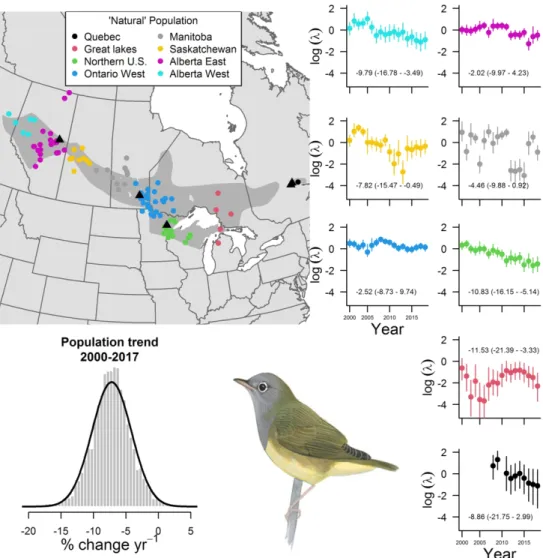
216 Across their range, the Connecticut warbler population declined by 8.99% (95% CI = -217 15.53 : -2.7) per year between 2000-2017 and is composed of eight ‘natural’ populations (Fig. 218 1.). Trend estimates indicate that all ‘natural’ populations are declining with mean trend
219 estimates ranging from -12.48% to -5.02% per year. The 95% credible interval for nearly half of 220 the ‘natural’ populations (n = 3 of 8) did not include zero indicating a statistically significant 221 decline (see Fig. 1.). Although the 95% credible interval overlapped zero for 5 of the 8 ‘natural’ 222 populations, between 88.42 and 99.97 percent of all samples drawn from the posterior
223 distribution (n = 9999) were negative trend estimates. 224 Migratory Connectivity
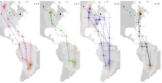
225 Connecticut warblers from the four tracked populations initiated fall migration in August 226 (Aug. 19 ± 5.28 days) and arrived on the east coast of North America in early September 227 (Sept. 10 ± 6.63 days). All but one Connecticut warbler made long-distance over water flights 228 from the east coast of North America on their way to South America. Individuals spent 10.5 ± 229 2.31 days on stopover prior to departing over the Atlantic in early October (Oct. 10 ± 5.82 days). 230 Mean flight time over the Atlantic Ocean was approximately 3 ± 0.65 days. Upon arrival to the 231 stopover in the Caribbean or South America, Connecticut warblers stayed on average 10.71 ± 232 2.43 days. They arrived on their stationary non-breeding grounds in early November (Nov. 09 ± 233 3.52 days), 81.5 ± 5.23 days after departing their breeding locations.
234 Connecticut warblers tended to have population specific stopover areas prior to and 235 immediately following their long-distance flights over the Atlantic. The strength of migratory 236 connectivity was stronger between breeding and fall stopover sites (stopover pre-Atlantic: MC = 237 0.24 ± 0.23, stopover post-Atlantic: MC = 0.31 ± 0.23) than it was between breeding and non-238 breeding grounds (MC = -0.2 ± 0.14). Most individuals spent the stationary non-breeding season 239 in an overlapping region of South America which includes southwestern Brazil, eastern Bolivia 240 and northern Paraguay (Fig. 2).
241 Habitat loss & fragmentation
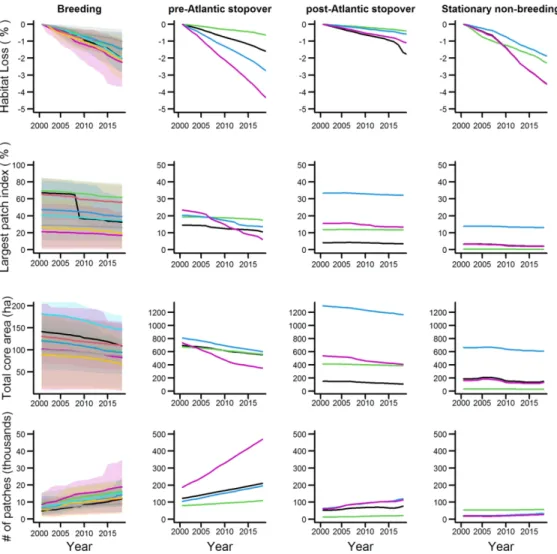
242 Habitat loss occurred within breeding, migratory stopover and stationary non-breeding areas 243 used by Connecticut warblers. The annual rate of habitat loss was greatest within the
non-244 breeding regions in South America (mean = -0.16; range = -0.21 to -0.11 % -yr) followed by
246 season (mean = -0.1; range = -0.13 to -0.06 % -yr), and finally stopover regions post Atlantic
247 crossing (mean = -0.05; range = -0.08 to -0.02 % -yr; Fig. 3).
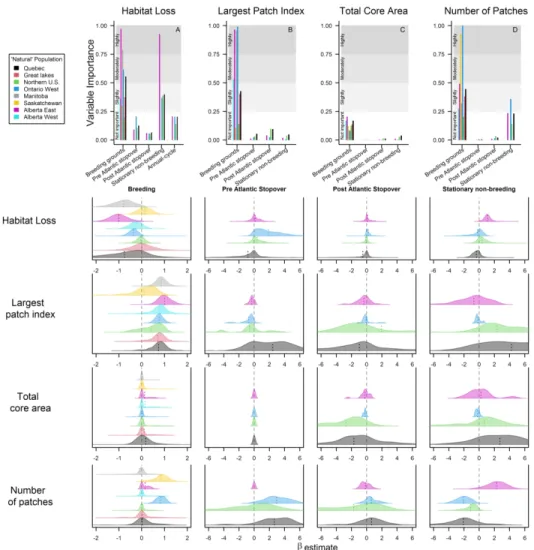
248 Connecticut warbler breeding abundance in 3 of 8 ‘natural’-populations was negatively 249 correlated with cumulative habitat loss within 50km of breeding locations (Fig. 4A) and was the 250 most important variable in the habitat loss model for 7 of the 8 populations. The effect of habitat 251 loss at stopover locations prior to and following crossing the Atlantic were not identified as 252 important contributors to Connecticut warbler abundance for any of the ‘natural’ populations 253 within our modeling framework ( < 0.25). Cumulative habitat loss during the stationary non-𝛾 254 breeding season in South America was identified as a highly important variable affecting 255 abundance in the Alberta East breeding population ( = 0.97) and slightly important (0.5 > > 𝛾 𝛾 256 0.25) for the remaining tracked populations (Ontario West: = 0.37; Northern U.S.: = 0.39; 𝛾 𝛾 257 and Québec: = 0.4). Habitat loss during the stationary non-breeding season was more important 𝛾 258 than breeding habitat loss for the Northern U.S. population but was not statistically significant ( 𝛽 259 = 0.15; 95% CI = -0.45 : 1.42, Fig. 4).
260 Habitat loss increased habitat fragmentation within the landscapes used by Connecticut 261 warblers throughout their annual cycle. Largest patch index (LPI) on the breeding grounds was 262 identified as an important variable in our fragmentation modeling framework, was positively 263 correlated with Connecticut warbler abundance and was statistically significant in nearly all 264 populations (Fig. 4). LPI was generally higher on the breeding grounds than within either 265 stopover region or on the stationary non-breeding grounds (Fig. 3). Despite the declines in total 266 core area (TCA) throughout the annual cycle, TCA was not identified as an important feature of 267 the landscape contributing to abundance on the breeding grounds (Fig. 4C). The number of
269 slightly ( > 0.25, n = 4 of 8 ‘natural’ populations) to highly important ( > 0.75, n = 2 of 8 𝛾 𝛾 270 ‘natural’ populations) for many of the sub-populations. Our modeling framework suggests that 271 the number of habitat patches (NP) during the stationary non-breeding period was more
272 important for abundance on the breeding grounds than the number of habitat patches within 273 landscapes that Connecticut warblers used during migratory stopover (Fig. 4D). The effect that 274 NP had on breeding abundance differed between the phases of the annual cycle. For example, the 275 number of habitat patches on the breeding grounds was positively correlated with breeding 276 abundance in the Saskatchewan ( = 0.83; 95% CI = 0 : 1.54) and Ontario West ( = 0.85; 95% 𝛽 𝛽 277 CI = 0.46 : 1.22) populations while the number of patches on the stationary non-breeding
278 grounds was negatively correlated with observed breeding abundance for the Québec ( = -0.49; 𝛽 279 95% CI = -4.72 : 0.4) and Ontario West ( = -0.75; 95% CI = -3.52 : 0) populations. The number 𝛽 280 of habitat patches during the stationary non-breeding period was positively correlated with 281 breeding ground abundance within the Alberta East population ( = 0.54; 95% CI = 0 : 3.79).𝛽 282 Discussion
283 Identifying the causes of population declines for migratory animals is an urgent yet 284 challenging objective for multiple reasons, not the least of which is we still lack essential 285 information on migratory connectivity for most species [2]. Here, we provide a framework that 286 integrates multiple data sources to identify where within the annual cycle environmental
287 perturbations impact migratory populations. Through the combined use of long-term community 288 science data (breeding bird surveys), tracking technology and remote sensing we found that 289 habitat loss and the resulting habitat fragmentation on the breeding grounds was most strongly 290 correlated with population declines for a steeply declining long-distance migratory songbird, the 291 Connecticut warbler.
292 The strength of migratory connectivity between breeding locations and key migratory 293 stopover regions was stronger than it was between breeding and non-breeding locations. Our 294 results suggest that during autumn, breeding populations use migratory routes unique to each 295 ‘natural’ population but winter in the same general region of South America. However, our 296 migratory connectivity inferences are based on tracking information from relatively few
297 individuals. The factors contributing to stronger migratory connectivity during fall migration are 298 unknown but profitable wind patterns may be responsible [43]. The synchronous timing of 299 departure (Oct. 10 ± 5.82 days) from eastern North America despite individuals breeding across 300 their range suggests that favorable wind patterns during long-distance over-water flights may 301 govern migration timing [44]. Prior to departing the east coast of North America individuals 302 spent on average 10.5 days on stopover. Although the need to maximize re-fueling rates is 303 important, the long duration on stopover may also indicate selection for favorable wind patterns 304 prior to making long-distance over-water flights [44].
305 Interestingly, several other steeply declining songbird species that breed in North America, 306 the Prothonotary warbler (Protonotaria citrea; [45]) and Purple Martin (Progne subis; [46]) 307 exhibit similar patterns of migratory connectivity where populations migrate along different 308 routes but winter in the same general location. Such a pattern could arise if survival varies
309 geographically within the non-breeding distribution [4,47]. If survival varies markedly across the 310 distribution, more individuals wintering in high survival locations will return to the breeding 311 grounds resulting in weak migratory connectivity, i.e., the appearance that individuals from 312 across the breeding distribution winter in a similar geographic region. Further research is needed 313 to determine how spatial variation in survival across the annual cycle could influence observed 314 migratory connectivity patterns [4]. However, the analytical framework employed here could be
315 used to help identify where within the annual cycle migratory populations are limited and could 316 be used for any migratory species where adequate tracking data and survey data exist.
317 Combining tracking technology and remote sensing allowed us to identify how habitat loss 318 and fragmentation at different times and places in the annual cycle correlates with population 319 declines observed during the breeding season. Our findings, although based on relatively few 320 tracked individuals suggest that habitat loss and fragmentation on the breeding grounds is 321 strongly correlated with population declines. Connecticut warblers exhibit weak migratory 322 connectivity between breeding and stationary non-breeding seasons, as such our ability to detect 323 a habitat loss or fragmentation signal from the non-breeding grounds is likely diminished. 324 Furthermore, more data were available from the breeding grounds and at a finer spatial
325 resolution (Breeding Bird Survey) than from the non-breeding phases of the annual cycle. The 326 combination of archival tracking technology with inherent location uncertainty and relatively 327 few tracked individuals may have decreased our ability to detect the full extent of how non-328 breeding season habitat loss and fragmentation impact Connecticut warbler abundance.
329 However, this study illustrates that tracking data combined with other data sources can improve 330 our understanding of the biology and threats to little-known species.
331 Tracking data were only available during autumn migration and the stationary non-332 breeding season, as such our findings do not consider the role of habitat loss in regions used 333 during spring migration on population dynamics. Connecticut warblers undertake large over-334 water flights during southward migration in autumn [27], and it is possible they use alternate 335 routes during their journey north in spring and are impacted by habitat loss in regions not 336 included in our analyses. However, community science (also referred to as citizen science) 337 observations submitted to eBird suggest that Connecticut warblers migrate primarily through the
338 Caribbean Basin and into eastern North America as they migrate north in the spring - the same 339 general regions used during fall we identified with light-level geolocators (Fig. S5). That said, 340 the evidence that habitat loss and resulting fragmentation on the breeding grounds is most
341 strongly correlated with on-going declines suggests it is likely an important contributing factor in 342 population declines.
343 Little is known about the basic biology of Connecticut warblers despite on-going population 344 declines (∼ 70% decline since 1966). For example, information as fundamental as the non-345 breeding distribution and patterns of habitat use are essentially undescribed in the scientific 346 literature [25,27]. The primary wintering locations identified here encompassed the northern 347 Gran Chaco ecoregion, a region including southern Brazil, eastern Bolivia, and northern 348 Paraguay, further south than previously thought although few observations and captures from 349 that region exist [25]. The Gran Chaco ecoregion is a global deforestation hotspot [35,48] and 350 lost >20% of it’s forest between 1985 and 2013 (142,000km2; [48]). Deforestation rate in the 351 region has increased substantially since 2000 [48]. Remotely sensed land cover data indicate the 352 region is dominated by savanna (37.28%), and grassland (23.65%) ecosystems. However, the 353 forested areas within the region where Connecticut warblers winter are comprised of deciduous 354 broadleaf (12.79%) and evergreen broadleaf (7.77%) forest types. Agriculture is common in the 355 region with croplands encompassing about 5% (4.39%) of the landscape. Commodity driven 356 deforestation and shifting agricultural practices are the dominant causes of permanent forest loss 357 in the region [49]. Continued expansion and further encroachment of agriculture could pose a 358 threat to these forested areas in future [48,50]. Inherent location uncertainty associated light-level 359 geolocation [34] precluded us from inferring habitat associations during the winter period.
361 support Connecticut warblers from across their breeding range. Therefore, continued forest loss 362 in the region will likely impact Connecticut warbler populations across their breeding
363 distribution. Currently, over 4,300 square kilometers of protected areas exist in the region where 364 they wintered including portions of the forested regions.
365 The breeding range of Connecticut warblers falls primarily within warm continental and 366 subarctic ecoregions, but specific habitat requirements differ across their breeding range [51]. In 367 the northwestern portion of their breeding distribution, they breed in upland aspen (Poplar sp.) 368 stands [52,53] while across most of their distribution they breed in wet, tamarack (Larix laricina) 369 / black spruce (Picea mariana) [54], and jack pine (Pinus banksiana) stands [55]. Cumulative 370 habitat loss within 50km of breeding bird survey routes had stronger effects on population 371 declines in areas where they breed in wet, tamarack / black spruce and jack pine stands. While 372 the underlying mechanism contributing to the observed differences between forest types are not 373 well understood, the potential regeneration time of the forest structure to a state needed for 374 successful reproduction may differ depending whether they breed in wet, tamarack stands or 375 upland aspen woodlands and may contribute to on-going population declines.
376 Habitat loss and the resulting fragmentation on the breeding grounds is strongly correlated 377 with observed population declines for the Connecticut warbler. Our findings suggest that large 378 intact forest patches within the landscape are positively correlated with Connecticut warbler 379 abundance. Therefore, Connecticut warbler populations would likely benefit from land
380 management practices that retain large, intact forest patches within the landscape. Although the 381 specific causes of habitat loss were not identified here, conversion of forest to agriculture 382 [56,57], peat mining [58] and forestry practices are common in the region and have impacts on 383 breeding bird species. Curtis et al. [49] found that forestry and wildfire are the primary sources
384 of forest cover loss within the warm continental and subarctic ecoregions in North America, but 385 most of these losses will recover with subsequent tree regrowth. However, these disturbances 386 affect forest age structure and composition that may result in habitat loss for the Connecticut 387 warbler. Forestry within the northern temperate / boreal forest is an important industry. In 388 Canada, where the vast majority of Connecticut warblers breed, the forestry industry employs 389 over 200,000 people and accounts for over 7% of all Canadian exports totaling over $25 billion 390 for the Canadian economy [59]. As such, without some immediate policy action for habitat 391 protection, the continued harvesting of forest products and resultant change in forest age
392 structure and composition will continue and may further influence declines of this poorly known 393 species.
394 Acknowledgements – This research is part of the Migratory Connectivity Project, funded by the
395 ConocoPhillips Charitable Investment Global Signature Program and the Natural Sciences and 396 Engineering Research Council of Canada (NSERC). We thank F. Hallworth, A. Hunt, J. 397 Kennedy, S. Stensaas, and D. Narango for assisting in the field. We thank K. Devarajan, A. 398 Sirén, M. Zimova, and four anonymous reviewers who provided valuable comments that 399 improved the manuscript.
400 Author Contributions – M.T.H. & P.P.M. conceived the idea for the manuscript. M.T.H., E.B.,
401 E.M., J.T., B.D., J.I., & P.P.M. conducted field work. M.T.H. conducted the analyses and wrote 402 the initial manuscript. All authors edited and approved of the final version of the manuscript. 403 Competing Interests – The authors declare no competing interests.
404 Data Availability – Movement data associated with the manuscript can be found in
405 movebank.org. Movebank ID = 613824346. Breeding bird survey data are available at 406 https://www.pwrc.usgs.gov/BBS/RawData/
407 Ethics – Animal handling protocols were approved by the Smithsonian’s National Zoological
408 Park International Animal Care and Use Committee (NZP-IACUC #17-05). 409 References
410 1. North American Bird Conservation Initiative. 2016 The State of North America’s Birds
411 2016.
412 2. Marra PP, Hunter D, Perrault AM. 2011 Migratory connectivity and the conservation of 413 migratory animals. Envtl. L. 41, 317.
414 3. Martin TG, Chadès I, Arcese P, Marra PP, Possingham HP, Norris DR. 2007 Optimal
415 Conservation of Migratory Species. PLOS ONE 2, e751. (doi:10.1371/journal.pone.0000751) 416 4. Rushing CS, Van Tatenhove AM, Sharp A, Ruiz-Gutierrez V, Freeman MC, Sykes PW, 417 Given AM, Sillett TS. 2020 Integrating tracking and resight data from breeding Painted 418 Bunting populations enables unbiased inferences about migratory connectivity and winter 419 range survival. (doi:10.1101/2020.07.23.217554)
420 5. Sorte FAL, Fink D, Blancher PJ, Rodewald AD, Ruiz‐Gutierrez V, Rosenberg KV, 421 Hochachka WM, Verburg PH, Kelling S. 2017 Global change and the distributional 422 dynamics of migratory bird populations wintering in Central America. Global Change 423 Biology 23, 5284–5296. (doi:10.1111/gcb.13794)
424 6. Rushing CS, Ryder TB, Marra PP. 2016 Quantifying drivers of population dynamics for a 425 migratory bird throughout the annual cycle. Proc. R. Soc. B 283, 20152846.
426 (doi:10.1098/rspb.2015.2846)
427 7. Kramer GR et al. 2018 Population trends in Vermivora warblers are linked to strong 428 migratory connectivity. PNAS 115, E3192–E3200. (doi:10.1073/pnas.1718985115) 429 8. Lambert JD, Hannon SJ. 2000 Short-Term Effects of Timber Harvest on Abundance, 430 Territory Characteristics, and Pairing Success of Ovenbirds in Riparian Buffer Strips. The 431 Auk 117, 687–698. (doi:10.2307/4089593)
432 9. Taylor CM, Stutchbury BJM. 2016 Effects of breeding versus winter habitat loss and 433 fragmentation on the population dynamics of a migratory songbird. Ecological Applications 434 26, 424–437. (doi:10.1890/14-1410)
435 10. Norris DR, Marra PP. 2007 Seasonal Interactions, Habitat Quality, and Population Dynamics 436 in Migratory Birds. The Condor 109, 535–547.
437 11. Dossman BC, Matthews SN, Rodewald PG. 2017 An experimental examination of the 438 influence of energetic condition on the stopover behavior of a Nearctic–Neotropical 439 migratory songbird, the American Redstart (Setophaga ruticilla). The Auk 135, 91–100. 440 (doi:10.1642/AUK-17-67.1)
441 12. Studds CE et al. 2017 Rapid population decline in migratory shorebirds relying on Yellow 442 Sea tidal mudflats as stopover sites. Nature Communications 8, 14895.
444 13. Rakhimberdiev E et al. 2018 Fuelling conditions at staging sites can mitigate Arctic warming 445 effects in a migratory bird. Nature Communications 9, 4263.
(doi:10.1038/s41467-018-446 06673-5)
447 14. Bridge ES et al. 2011 Technology on the Move: Recent and Forthcoming Innovations for 448 Tracking Migratory Birds. BioScience 61, 689–698.
449 15. Stutchbury BJM, Tarof SA, Done T, Gow E, Kramer PM, Tautin J, Fox JW, Afanasyev V. 450 2009 Tracking long-distance songbird migration by using geolocators. Science 323, 896. 451 16. McKinnon EA, Love OP. 2018 Ten years tracking the migrations of small landbirds: 452 Lessons learned in the golden age of bio-logging. The Auk 135, 834–856.
453 (doi:10.1642/AUK-17-202.1)
454 17. Bridge ES, Kelly JF, Contina A, Gabrielson RM, MacCurdy RB, Winkler DW. 2013 455 Advances in tracking small migratory birds: a technical review of light-level geolocation. 456 Journal of Field Ornithology 84, 121–137. (doi:10.1111/jofo.12011)
457 18. Heckscher CM, Taylor SM, Fox JW, Afanasyev V. 2011 Veery (Catharus fuscescens) 458 Wintering Locations, Migratory Connectivity, and a Revision of its Winter Range Using 459 Geolocator Technology. The Auk 128, 531–542. (doi:10.1525/auk.2011.10280)
460 19. Hallworth MT, Marra PP. 2015 Miniaturized GPS Tags Identify Non-breeding Territories of 461 a Small Breeding Migratory Songbird. Scientific Reports 5, 11069. (doi:10.1038/srep11069)
462 20. Cooper NW, Hallworth MT, Marra PP. 2017 Light-level geolocation reveals wintering 463 distribution, migration routes, and primary stopover locations of an endangered long-distance 464 migratory songbird. J Avian Biol 48, 209–219. (doi:10.1111/jav.01096)
465 21. Hallworth MT, Sillett TS, Van Wilgenburg SL, Hobson KA, Marra PP. 2015 Migratory 466 connectivity of a Neotropical migratory songbird revealed by archival light-level 467 geolocators. Ecological Applications 25, 336–347. (doi:10.1890/14-0195.1) 468 22. Cohen EB, Hostetler JA, Hallworth MT, Rushing CS, Sillett TS, Marra PP. 2018
469 Quantifying the strength of migratory connectivity. Methods in Ecology and Evolution 9, 470 513–524. (doi:10.1111/2041-210X.12916)
471 23. Fraser KC et al. 2012 Continent-wide tracking to determine migratory connectivity and 472 tropical habitat associations of a declining aerial insectivore. Proc. R. Soc. B 279, 4901– 473 4906. (doi:10.1098/rspb.2012.2207)
474 24. Sheehy J, Taylor CM, Norris DR. 2011 The importance of stopover habitat for developing 475 effective conservation strategies for migratory animals. J Ornithol 152, 161–168.
476 (doi:10.1007/s10336-011-0682-5)
477 25. Pitocchelli J, Jones J, Jones D, Bouchie J. 2020 Connecticut Warbler (Oporornis agilis). 478 Birds of the World
479 26. Sauer JR, Link WA, Hines JE. 2020 The North American Breeding Bird Survey, Analysis 480 Results 1966 - 2019. (doi:10.5066/P96A7675)
481 27. McKinnon EA, Artuso C, Love OP. 2017 The mystery of the missing warbler. Ecology 98, 482 1970–1972. (doi:10.1002/ecy.1844)
483 28. Rushing CS, Ryder TB, Scarpignato AL, Saracco JF, Marra PP. 2016 Using demographic 484 attributes from long-term monitoring data to delineate natural population structure. Journal 485 of Applied Ecology 53, 491–500. (doi:10.1111/1365-2664.12579)
486 29. Brlík V et al. 2020 Weak effects of geolocators on small birds: A meta-analysis controlled 487 for phylogeny and publication bias. Journal of Animal Ecology 89, 207–220.
488 (doi:10.1111/1365-2656.12962)
489 30. Wotherspoon S. 2017 SGAT: Solar/Satellite Geolocation for Animal Tracking. See 490 https://github.com/SWotherspoon/SGAT.
491 31. Sumner MD, Wotherspoon SJ, Hindell MA. 2009 Bayesian Estimation of Animal Movement 492 from Archival and Satellite Tags. PLOS ONE 4, e7324. (doi:10.1371/journal.pone.0007324) 493 32. R Core Team. 2017 R: A language and environment for statistical computing. R Foundation 494 for Statistical Computing. Vienna, Austria. See https://www.R-project.org/.
495 33. Hostetler J, Hallworth MT. 2018 MigConnectivity: v0.3.0. Zenodo. 496 (doi:10.5281/zenodo.1306198)
497 34. Lisovski S et al. 2018 Inherent limits of light-level geolocation may lead to over-498 interpretation. Current Biology 28, R99–R100. (doi:10.1016/j.cub.2017.11.072)
499 35. Hansen MC et al. 2013 High-Resolution Global Maps of 21st-Century Forest Cover Change. 500 Science 342, 850–853. (doi:10.1126/science.1244693)
501 36. Gorelick N, Hancher M, Dixon M, Ilyushchenko S, Thau D, Moore R. 2017 Google Earth 502 Engine: Planetary-scale geospatial analysis for everyone. Remote Sensing of Environment 503 202, 18–27. (doi:10.1016/j.rse.2017.06.031)
504 37. Wang X, Blanchet FG, Koper N. 2014 Measuring habitat fragmentation: An evaluation of 505 landscape pattern metrics. Methods in Ecology and Evolution 5, 634–646.
506 (doi:10.1111/2041-210X.12198)
507 38. Hesselbarth MHK, Sciaini M, With KA, Wiegand K, Nowosad J. 2019 landscapemetrics: an 508 open-source R tool to calculate landscape metrics. Ecography 42, 1648–1657.
509 (doi:10.1111/ecog.04617)
510 39. Hooten MB, Hobbs NT. 2015 A guide to Bayesian model selection for ecologists. Ecological 511 Monographs 85, 3–28. (doi:10.1890/14-0661.1)
512 40. Plummer M. 2003 JAGS: A program for analysis of Bayesian graphical models using Gibbs 513 sampling. In Proceedings of the 3rd international workshop on distributed statistical
514 computing, p. 125. Vienna, Austria.
515 41. Kellner K. 2016 jagsUI: a wrapper around rjags to streamline JAGS analyses. R package 516 version 1.
517 42. Kéry M, Royle JA. 2016 Applied Hierarchical Modeling in Ecology: Analysis of
518 distribution, abundance and species richness in R and BUGS - 1st Edition. Academic Press. 519 43. Kranstauber B, Weinzierl R, Wikelski M, Safi K. 2015 Global aerial flyways allow efficient 520 travelling. Ecol Lett 18, 1338–1345. (doi:10.1111/ele.12528)
521 44. McLaren JD, Shamoun-Baranes J, Bouten W. 2012 Wind selectivity and partial
522 compensation for wind drift among nocturnally migrating passerines. Behav Ecol 23, 1089– 523 1101. (doi:10.1093/beheco/ars078)
524 45. Tonra CM et al. 2019 Concentration of a widespread breeding population in a few critically 525 important nonbreeding areas: Migratory connectivity in the Prothonotary Warbler. Condor 526 121. (doi:10.1093/condor/duz019)
527 46. Fraser KC et al. 2013 Consistent range-wide pattern in fall migration strategy of Purple 528 Martin (Progne subis), despite different migration routes at the Gulf of Mexico. The Auk 529 130, 291–296. (doi:10.1525/auk.2013.12225)
530 47. Ruiz-Gutiérrez V, Doherty PF, Eduardo Santana C, Martínez SC, Schondube J, Munguía 531 HV, Iñigo-Elias E. 2012 Survival of Resident Neotropical Birds: Considerations for 532 Sampling and Analysis Based on 20 Years of Bird-Banding Efforts in Mexico. Auk 129, 533 500–509. (doi:10.1525/auk.2012.11171)
534 48. Baumann M, Gasparri I, Piquer‐Rodríguez M, Pizarro GG, Griffiths P, Hostert P,
535 Kuemmerle T. 2017 Carbon emissions from agricultural expansion and intensification in the 536 Chaco. Global Change Biology 23, 1902–1916. (doi:https://doi.org/10.1111/gcb.13521) 537 49. Curtis PG, Slay CM, Harris NL, Tyukavina A, Hansen MC. 2018 Classifying drivers of 538 global forest loss. Science 361, 1108–1111. (doi:10.1126/science.aau3445)
539 50. Romero-Muñoz A et al. 2019 Habitat loss and overhunting synergistically drive the 540 extirpation of jaguars from the Gran Chaco. Divers Distrib 25, 176–190.
542 51. Solymos P, Stralberg D. 2020 BAM Generalized National Models Documentation, Version 543 4.0. (doi:10.5281/zenodo.4042821)
544 52. Schieck J, Song SJ. 2006 Changes in bird communities throughout succession following fire 545 and harvest in boreal forests of western North America: literature review and meta-analyses. 546 Can. J. For. Res. 36, 1299–1318. (doi:10.1139/x06-017)
547 53. Kirk DA, Diamond AW, Hobson KA, Smith AR. 1996 Breeding bird communities of the 548 western and northern Canadian boreal forest: relationship to forest type. Can. J. Zool. 74, 549 1749–1770. (doi:10.1139/z96-193)
550 54. Lapin CN, Etterson MA, Niemi GJ. 2013 Occurrence of the Connecticut Warbler increases 551 with size of patches of coniferous forest. The Condor 115, 168–117.
552 (doi:10.1525/cond.2013.110202)
553 55. Blais V. 2014 Caractérisation et utilisation de l’habitat par la Paruline à gorge grise 554 (Oporornis agilis) dans les pinèdes grises du Lac-Saint-Jean, Québec. M.Sc. Thesis 555 Université du Québec à Chicoutimi.
556 56. Hobson KA, Bayne EM, Van Wilgenburg SL. 2002 Large-scale conversion of forest to 557 agriculture in the boreal plains of Saskatchewan. Conservation Biology 16, 1530–1541. 558 (doi:10.1046/j.1523-1739.2002.01199.x)
559 57. Young JE, Sánchez-Azofeifa GA, Hannon SJ, Chapman R. 2006 Trends in land cover 560 change and isolation of protected areas at the interface of the southern boreal mixedwood 561 and aspen parkland in Alberta, Canada. Forest Ecology and Management 230, 151–161.
563 58. Desrochers A, Rochefort L, Savard J-PL. 1998 Avian recolonization of eastern Canadian 564 bogs after peat mining. Can. J. Zool. 76, 989–997. (doi:10.1139/z98-028)
565 59. Canada NR. 2014 How does the forest industry contribute to Canada’s economy? See 566 https://www.nrcan.gc.ca/forests/report/economy/16517 (accessed on 15 November 2018). 567
568 Tables
569 Table 1. coefficients between forest loss during different phases of the annual cycle and Connecticut warbler abundance on the 𝛽 570 breeding grounds. Connecticut warbler ‘natural’ populations were identified following [30]. Mean correlations are shown along with 𝛽 571 the 95% credible interval in parenthesis. Zero values are reported outside of the breeding season for ‘natural’ populations with no 572 tracking data. The number of Breeding Bird Survey routes the comprise the ‘natural’ population are reported in parentheses.
‘Natural’ Population Breeding Pre-Atlantic Post-Atlantic
Stationary non-breeding Cumulative Québec (n = 1) -0.76 (-3.49 : 0.86) -0.83 (-6.44 : 2.67) -0.5 (-4.12 : 0.83) -0.36 (-1.49 : 0.73) -0.16 (-0.86 : 0.24) Great Lakes (n = 5) 0.01 (-1.00 : 1.04) Ontario West (n = 26) -0.04 (-0.43 : 0.30) 0.37 (-1.18 : 2.32) -0.13 (-1.21 : 0.42) 0.39 (-0.73 : 1.87) -0.01 (-0.31 : 0.25) Northern U.S. (n = 13) -0.36 (-0.80 : 0.04) 1.86 (-0.07 : 5.61) 0.19 (-0.27 : 1.20) -0.22 (-2.43 : 0.88) -0.05 (-0.76 : 0.48) Alberta W. (n = 6) -0.26 (-0.81 : 0.27) Alberta E. (n = 20) -1.01 (-1.74 : -0.20) 0.11 (-1.09 : 1.32) 0.12 (-0.73 : 1.20) 1.09 (0.15 : 2.11) -0.01 (-0.72 : 0.51) Saskatchewan (n = 9) 0.14 (-0.40 : 0.70) Manitoba (n = 10) -0.80 (-1.79 : 0.01) 573
574 Table 2. coefficients for three habitat fragmentation parameters, total core area (TCA), number of patches (NP) and largest patch 𝛽 575 index (LPI) throughout the annual cycle on Connecticut warbler abundance on the breeding grounds. The mean effect size along with 576 the 95% credible interval are reported. coefficients where the 95% credible interval does not include zero are indicated with bold 𝛽 577 font. The effect sizes outside the breeding season are reported as zero for ‘natural’ populations without tracking data.
Fragmentation
Metric Québec Great Lakes Ontario West Northern U.S. Alberta W. Alberta E. Saskatchewan Manitoba
Total Core Area
Breeding 1.03 (-0.5:7.28) 0.34 (-0.54:1.15) 0.33 (-0.5:1.09) 0.08 (-0.63:0.63) 0.40 (-0.08:0.93) 0.41 (0.06:0.78) 0.37 (-0.25:1.34) 0.19 (-0.43:0.69) Pre-Atlantic 0 0 0 0 Post-Atlantic -1.68 (-10.48:4.62) -2.72 (-9.44:0.36) -0.24 (-0.49:-0.01) -0.24 (-1.74:0.54) Stationary Non-breeding 2.72 (-3.8:9.99) 0.65 (-5.76:5.3) -0.22 (-0.5:0.14) 0.22 (-2.21:4.48) Number of Patches
Breeding -0.47 (-4.53:1.31) 0.3 (-2.91:1.19) 0.03 (-0.84:0.8) 0.85 (0.46:1.22) 0.08 (-1.15:1.06) 0.29 (0.05:0.55) 0.89 (0.29:1.56) 0.39 (-1.74:0.81) Pre-Atlantic 0.01 (0:0) 0 (0:0) 0.02 (0:0) 0 (0:0) Post-Atlantic 0.64 (-3.73:3.91) -1.72 (-9.16:3.37) 0.63 (-0.73:2.26) -0.16 (-1.02:0.86) Stationary Non-breeding -2.11 (-7.29:2.69) -1.13 (-3.41:0.02) -2.09 (-3.98:-0.51) 2.29 (-0.23:4.53) Largest Patch Index Breeding 0.74 (-0.23:1.41) 0.71 (-0.19:1.29) 0.43 (-0.61:1.12) 0.76 (0.42:1.13) 0.79 (-0.02:1.5) 1 (0.46:1.59) 0.11 (-1.68:0.92) 0.85 (0.38:1.33) Pre-Atlantic 0.13 (0:2.54) -0.02 (0:0) -0.02 (0:0) 0 (0:0) Post-Atlantic -0.96 (-9.12:8.13) 1.95 (-5.39:21.17) -0.07 (-1.02:2.05) -0.37 (-2.61:1.35) Stationary 4.22 2.33 -0.14 -0.71
579 Fig. 1 The breeding distribution of the Connecticut warbler (gray polygon) is comprised of eight
580 ‘natural’ populations. The breeding bird survey locations within each ‘natural’ population are 581 represented by different colors. The population trend and 95% credible interval are provided 582 alongside the abundance estimates for each ‘natural’ population. The population wide trend 583 estimate is also shown. The locations of light-level geolocator deployment are illustrated with a 584 black triangle. Image of Connecticut warbler drawn by David Sibley.
585 Fig. 2 Breeding, autumn migratory stopover regions and non-breeding locations of Connecticut
586 warblers captured throughout their breeding distribution. The four ‘natural’ populations, the 587 median (colored circles) and 95% credible intervals for each location during autumn migration 588 are shown. The stationary non-breeding location of individuals is indicated with a grey filled 589 point. Sample sizes are shown in each panel. Each individual track is connected with a dotted 590 line to distinguish between individuals but does not represent the actual path traveled between 591 stopover locations. The underlying color ramp represents the uncertainty for the tracking 592 duration.
593 Fig. 3 Habitat loss and fragmentation metrics across phases of the annual cycle of Connecticut
594 warblers. Cumulative forest loss (% change per year) is shown in the top row. The shaded area 595 around breeding season estimates represents the 95% CI for each ‘natural’ population. The colors 596 of the lines correspond to the ‘natural’ populations illustrated in Fig. 1. Although it appears in 597 some figures that fewer than four lines are present, three of the four populations wintered in the 598 same area and therefore have similar forest loss values. The three landscape fragmentation 599 metrics used in our analyses, largest patch index (LPI), total core area (TCA) and number of 600 forest patches (NP) are also shown. Landscape metrics were derived from the Global Forest
601 Change data set (version 1.6; [35]) using the LandscapeMetrics R package [38]. Note the 602 different scale of the y-axis in the breeding ground figures.
603 Fig. 4 The relative importance of forest loss and forest fragmentation metrics on population
604 declines of Connecticut warblers (A) and the posterior distribution of the coefficients (B). 𝛽 605 Indicator values approximating 1 indicate the variable is highly important while values
606 approximating 0 indicate the variable is not important. The colors of the posterior distributions 607 correspond to the ‘natural’ populations illustrated in Fig. 1. Indicator variable and estimates for 𝛽 608 the effect of forest loss outside of the breeding grounds are shown for only the populations 609 tracked via light-level geolocators.
Fig. 1 The breeding distribution of the Connecticut warbler (gray polygon) is comprised of eight ‘natural’ populations. The breeding bird survey locations within each ‘natural’ population are represented by different
colors. The population trend and 95% credible interval are provided alongside the abundance estimates for each ‘natural’ population. The population wide trend estimate is also shown. The locations of light-level geolocator deployment are illustrated with a black triangle. Image of Connecticut warbler drawn by David
Sibley.
Fig. 2 Breeding, autumn migratory stopover regions and non-breeding locations of Connecticut warblers captured throughout their breeding distribution. The four ‘natural’ populations, the median (colored circles)
and 95% credible intervals for each location during autumn migration are shown. The stationary non-breeding location of individuals is indicated with a grey filled point. Sample sizes are shown in each panel.
Each individual track is connected with a dotted line to distinguish between individuals but does not represent the actual path traveled between stopover locations. The underlying color ramp represents the
uncertainty for the tracking duration. 203x101mm (300 x 300 DPI)
Fig. 3 Habitat loss and fragmentation metrics across phases of the annual cycle of Connecticut warblers. Cumulative forest loss (% change per year) is shown in the top row. The shaded area around breeding season estimates represents the 95% CI for each ‘natural’ population. The colors of the lines correspond to
the ‘natural’ populations illustrated in Fig. 1. Although it appears in some figures that fewer than four lines are present, three of the four populations wintered in the same area and therefore have similar forest loss values. The three landscape fragmentation metrics used in our analyses, largest patch index (LPI), total core
area (TCA) and number of forest patches (NP) are also shown. Landscape metrics were derived from the Global Forest Change data set (version 1.6; [35]) using the LandscapeMetrics R package [38]. Note the
different scale of the y-axis in the breeding ground figures. 101x101mm (300 x 300 DPI)
Fig. 4 The relative importance of forest loss and forest fragmentation metrics on population declines of Connecticut warblers (A) and the posterior distribution of the \beta coefficients (B). Indicator values approximating 1 indicate the variable is highly important while values approximating 0 indicate the variable
is not important. The colors of the posterior distributions correspond to the ‘natural’ populations illustrated in Fig. 1. Indicator variable and β estimates for the effect of forest loss outside of the breeding grounds are
shown for only the populations tracked via light-level geolocators. 203x203mm (300 x 300 DPI)