Publisher’s version / Version de l'éditeur:
Vous avez des questions? Nous pouvons vous aider. Pour communiquer directement avec un auteur, consultez
la première page de la revue dans laquelle son article a été publié afin de trouver ses coordonnées. Si vous n’arrivez pas à les repérer, communiquez avec nous à [email protected].
Questions? Contact the NRC Publications Archive team at
[email protected]. If you wish to email the authors directly, please see the first page of the publication for their contact information.
https://publications-cnrc.canada.ca/fra/droits
L’accès à ce site Web et l’utilisation de son contenu sont assujettis aux conditions présentées dans le site LISEZ CES CONDITIONS ATTENTIVEMENT AVANT D’UTILISER CE SITE WEB.
Proceedings of the Canadian AI-2006 Conference, 2006
READ THESE TERMS AND CONDITIONS CAREFULLY BEFORE USING THIS WEBSITE. https://nrc-publications.canada.ca/eng/copyright
NRC Publications Archive Record / Notice des Archives des publications du CNRC :
https://nrc-publications.canada.ca/eng/view/object/?id=5a784356-33bb-4f49-9ddc-79ca68bde2d8
https://publications-cnrc.canada.ca/fra/voir/objet/?id=5a784356-33bb-4f49-9ddc-79ca68bde2d8
NRC Publications Archive
Archives des publications du CNRC
This publication could be one of several versions: author’s original, accepted manuscript or the publisher’s version. / La version de cette publication peut être l’une des suivantes : la version prépublication de l’auteur, la version acceptée du manuscrit ou la version de l’éditeur.
Access and use of this website and the material on it are subject to the Terms and Conditions set forth at
Learning Naive Bayes Tree for Conditional Probability Estimation
National Research Council Canada Institute for Information Technology Conseil national de recherches Canada Institut de technologie de l'information
Learning Naive Bayes Tree for Conditional
Probability Estimation *
Liang, H., and Yan, Y.
June 2006
* published in the Proceedings of the Canadian AI-2006 Conference. Québec, Québec, Canada. June 7-9, 2006. Springer LNCS4013, pp. 456-466. Editors: L. Lamontagne, M. Marchand. NRC 48488.
Copyright 2006 by
National Research Council of Canada
Permission is granted to quote short excerpts and to reproduce figures and tables from this report, provided that the source of such material is fully acknowledged.
Learning Na¨ıve Bayes Tree for Conditional
Probability Estimation
Han Liang1⋆, Yuhong Yan2⋆⋆
1Faculty of Computer Science, University of New Brunswick
Fredericton, NB, Canada E3B 5A3
2 National Research Council of Canada
Fredericton, NB, Canada E3B 5X9 [email protected]
Abstract. Na¨ıve Bayes Tree uses decision tree as the general struc-ture and deploys na¨ıve Bayesian classifiers at leaves. The intuition is that na¨ıve Bayesian classifiers work better than decision trees when the sample data set is small. Therefore, after several attribute splits when constructing a decision tree, it is better to use na¨ıve Bayesian classifiers at the leaves than to continue splitting the attributes. In this paper, we propose a learning algorithm to improve the conditional probability es-timation in the diagram of Na¨ıve Bayes Tree. The motivation for this work is that, for cost-sensitive learning where costs are associated with conditional probabilities, the score function is optimized when the esti-mates of conditional probabilities are accurate. The additional benefit is that both the classification accuracy and Area Under the Curve (AUC) could be improved. On a large suite of benchmark sample sets, our ex-periments show that the CLL tree outperforms the state-of-art learning algorithms, such as Na¨ıve Bayes Tree and na¨ıve Bayes significantly in yielding accurate conditional probability estimation and improving clas-sification accuracy and AUC.
1
Introduction
Classification is a fundamental issue of machine learning in which a classifier is induced from a set of labeled training samples represented by a vector of attribute values and a class label. We denote attribute set A = {A1, A2, . . . , An}, and an assignment of value to each attribute in A by a corresponding bold-face lower-case letter a. We use C to denote the class variable and c to denote its value. Thus, a training sample is represented as E = (a, c), where a = (a1, a2, . . . , an), and ai is the value of attribute Ai. A classifier is a function f that maps a sample E to a class label c, i.e. f (a) = c. The inductive learning algorithm returns a function h that approximates f . The function h is called a hypothesis.
⋆The author is a visiting worker at NRC-IIT
⋆⋆ The authors thank Dr. Harry Zhang and Jiang Su from University of New Brunswick
The classifier can predict the assignment of C for an unlabeled testing sample Et= (b), i.e. h(b) = ct.
Various inductive learning algorithms, such as decision trees, Bayesian net-works, and neural netnet-works, can be categorized into two major approaches: probability-based approach and decision boundary-based approach. In a genera-tive probability learning algorithm, a probability distribution p(A, C) is learned from the training samples as a hypothesis. Then we can theoretically compute the probability of any E in the probability space. A testing sample Et= (b) is classified into the class c with the maximum posterior class probability p(c|b) (or simply class probability), as shown below.
h(b) = arg max
c∈C p(c|b) = arg maxc∈C p(c, b)/p(b) (1) Decision tree learning algorithms are well known as decision boundary-based. Though their probability estimates are poor, the algorithms can make good de-cisions on which side of the boundary a sample data falls. Decision trees work better when the sample data set is large. It is because, after several splits of at-tributes, the number of samples at the subspaces is too few on which to base the decision, while na¨ıve Bayesian classifier works better in this case. Therefore, in-stead of continuing to split the attributes, na¨ıve Bayesian classifiers are deployed at the leaves. [5] proposed this hybrid model called Na¨ıve Bayes Tree (NBTree). It is reported that NBTree outperforms C4.5 and na¨ıve Bayes in classification accuracy and AUC.
In this paper, we propose to use NBTree to improve the conditional proba-bility estimation given the support attributes, i.e. p(C|A). Accurate conditional probability is important in many aspects. First, in cost-sensitive classification, knowing the accurate conditional probability is crucial in making a decision. Determining only the decision boundary is not enough. Second, improving con-ditional probability can possibly improve classification accuracy, though it is not a necessary condition. Third, improving conditional probability can improve AUC which is a metric used for ranking.
Our proposed learning algorithm is a greedy and recursive procedure similar to NBTree. In each step of expanding the decision tree, the Conditional Log Likelihood (CLL) is used as the score function to select the best attribute to split, where let the CLL of a classifier B, given a (sub) sample set S be
CLL(B|S) = n X s=1
log PB(C|A) (2)
The splitting process ends when some conditions are met. Then for the sam-ples at leaves, na¨ıve Bayesian classifiers are generated. We call the generated tree CLL Tree (CLLTree). We present that on a large suite of benchmark sam-ple sets, our empirical results show that CLLTree significantly outperforms the state-of-art learning algorithms, such as NBTree and na¨ıve Bayes in yielding accurate probability estimation, classification accuracy and AUC.
2
Related Work in Decision Tree Probability Estimation
The probability generated from decision tree is calculated from the sub sample sets at leaves corresponding to the conjunction of the conditions along the paths back to the root [8]. Assume a leaf node defines a subset of 100 samples, 90 of which are in the positive class and others are in the negative class, then each sample is assigned the same probability of 0.9 (90/100) that it belongs to the positive class, i.e. ˆp(+|Ap = ap) = 90%, where Ap is the set of attributes on the path. Viewed as probability estimators, decision trees consist of piecewise uniform approximations within regions defined by axis-paralleled boundaries. Aiming at this fact, [8] presented two methods to improve the probability esti-mation of decision tree. First, by using Laplace estiesti-mation, probability estimates can be smoothed from small sample data at the tree leaves. Second, by turning off pruning and “collapsing” in C4.5, decision trees can generate finer trees to give more precise probability estimation. The final version is called C4.4.
Another improvement to tackle the “uniform probability distribution” lem of decision trees is to stop splitting at a certain level and put another prob-ability density estimator at each leaf. [5] proposed an NBTree that uses decision tree as the general structure and deploys na¨ıve Bayes classifiers at the leaves. This learning algorithm first uses classification accuracy as the score function to do univariate splits and when splitting does not increase the score function, a na¨ıve Bayesian classifier is created at the leaf. Thus, sample attributes are divided into two sets: A = Ap∪ Al, where Apis the set of path attributes and Alis the set of leaf attributes. [10] proposed one encode of p(C, A) for NBTree. The proposed Conditional Independent Tree (CITree) denotes p(A, C) as below: p(A, C) = αp(C|Ap(L))p(Al(L)|Ap(L), C) (3) where α is a normalization factor. The term p(C|Ap(L)) is the joint condi-tional distribution of path attributes and the term p(Al(L)|Ap(L), C) is the leaf attributes presented by na¨ıve Bayes p(Al|Ap(L), C) = Qni=1p(Ali|Ap(L), C). CITree explicitly defines conditional dependence among the path attributes and independence among the leaf attributes. The local conditional independence sumption of CITree is a relaxation of the (global) conditional independence as-sumption of na¨ıve Bayes.
Building decision trees with accurate probability estimation, called Probabil-ity Estimation Trees (PETs), has received a great deal of attention recently [8]. The difference of PET and CITree is that PET represents the conditional prob-ability distribution of the path attributes, while a CITree represents a joint distribution over all attributes.
Another related work involves Bayesian networks [7] which are directed acyclic graphs that encode conditional independence among a set of random variables. Each variable is independent of its non-descendants in the graph given the state of its parents. Tree Augmented Na¨ıve Bayes (TAN) [3] approximates the interaction between attributes by using a tree structure imposed on the na¨ıve Bayesian framework. We point out that, although TAN takes advantage
of tree structure, it is not a decision tree. Indeed, decision trees divide a sample space into multiple subspaces and local conditional probabilities are independent among those subspaces. Therefore, attributes in decision trees can repeatedly appear, while TAN describes the joint probabilities among attributes, so each attribute appears only once. In decision trees, p(C|A) is decomposable when a (sub) sample set is split into subspaces, but it is non-decomposable in TAN.
3
Learning Na¨ıve Bayes Tree for Conditional Probability
Estimation
In this section, we present our work on improving conditional probability esti-mation of na¨ıve Bayes Tree. First, we select the evaluation metrics. Second, we present the principles of representing CLL in CLL Tree. Last, we present a new algorithm for learning the na¨ıve Bayes tree.
3.1 The performance evaluation metrics
Accurate conditional probability p(C|A) is important for many applications. Since it is justified that log p is a monotonic function of p and we use conditional log likelihood (CLL) for calculation, we mix the usage of CLL and conditional probability hereafter. In cost-sensitive classification, the optimal prediction for a sample b is the class ci that minimize [2]
h(b) = arg min ci∈C
X cj∈C−ci
p(cj|b)C(ci, cj) (4) One can see that the score function in cost-sensitive learning directly relies on the conditional probability. It is not like the classification problem where only the decision boundary is important. Accurate estimation of conditional probability is necessary for cost-sensitive learning.
Better conditional probability estimation means better classification accuracy (ACC) (c.f. Equation 1). ACC is calculated as the percentage of the correctly classified samples over all the samples: ACC = 1
N P
I(h(a) = c), here N is the number of samples. However, improving conditional probability estimation is not a necessary condition for improving ACC. ACC can be scaled up through other ways, e.g. boundary-based approaches. On the other side, even if conditional probability is greatly improved, it may still lead to wrong classification.
Ranking is different from both classification and probability estimation. For example, assume that E+ and E− are a positive and a negative sample respec-tively, and that the actual class probabilities are p(+|E+) = 0.9 and p(−|E−) = 0.1. An algorithm that gives class probability estimates ˆp(+|E+) = 0.55 and ˆ
p(+|E−) = 0.54, gives a correct order of E+ and E− in the ranking. Notice that the probability estimates are poor and the classification for E− is incorrect. However, if a learning algorithm produces accurate class probability estimates, it certainly produces a precise ranking. Thus, aiming at learning a model to yield
accurate conditional probability estimation will usually lead to a model yielding precise probability-based ranking.
In this paper, we use three different metrics CLL, ACC and AUC to evaluate learning algorithms.
3.2 The representation of CLL in CLLTree
The representation of conditional probability in the diagram of CLLTree is as follows:
log(p(C|A)) = log(p(C|Al, Ap) = log(p(C|Ap))+log(p(Al|C, Ap))−log(p(Al|Ap)) (5) Ap divides a (sub) sample set into several subsets. All decomposed terms are the conditional probability of Ap. p(C|Ap) is the conditional probability on the path attributes; p(Al|C, Ap) is the na¨ıve Bayesian classifier at a leaf; and p(Al|Ap) is the joint probability of Al under condition of Ap.
In each step of generating the decision tree, CLL is calculated based on Equation 5. Assuming Ali denotes a leaf attribute, here, p(C|Ap) is calculated by the ratio of the number of samples that have the same class value to all the samples at a leaf; p(Al|C, Ap) can be represented by
Qm
i=1p(Ali|C, Ap) (m is the number of attributes at a leaf node), and each p(Ali|C, Ap) can be calculated by the ratio of the number of samples that have the same attribute value of Ali and the same class value to the number of samples that have the same class value; likewise, p(Al|Ap) can also be represented by
Qm
i=1p(Ali|Ap), and each p(Ali|Ap) can be calculated by the ratio of the number of samples that have the same attribute value of Ali to the number of samples at that leaf. The attribute to optimize CLL is selected as the next level node to extend the tree. We exhaustively build all possible trees in each step and keep only the best on for the next level expansion. Supposing finite k attributes are available. When expanding the tree at level q, there are k − q + 1 attributes to be chosen. This is a greedy way. CLLTree makes an assumption on probability, i.e. the probability dependency on the path attributes and the probability independency on the leaf attributes. Besides, it also has another assumption on the structure that each node has only one parent.
3.3 A New Algorithm for Learning CLLTree
From the discussion in the previous sections, CLLTree can represent any joint distribution. Therefore, the probability estimation based on CLLTree is accurate. But the structure learning of a CLLTree could theoretically be as time-consuming as learning an optimal decision tree. A good approximation of a CLLTree, which gives relatively accurate estimates of class probabilities, is desirable in many applications. Similar to a decision tree, building a CLLTree could be a greedy and recursive process. On each iteration, choose the “best” attribute as the root of the (sub) tree, split the associated data into disjoint subsets corresponding to the values of that attribute, and recur this process for each subset until certain
criteria are satisfied. If the structure of a CLLTree is determined, a leaf na¨ıve Bayes is a perfect model to represent the local conditional distribution at leaves. The algorithm is described below.
Algorithm 1Learning Algorithm CLLT ree(T, S, A) T : CLLTree
S: a set of labeled samples A: a set of attributes
foreach attribute a ∈ A do
Partition S into S1, S2, ..., Sk, where k is the number of possible values of attribute a. Each sub set is corresponding to a value of a. For continuous attributes, a threshold is set up in this step.
Create a na¨ıve Bayes for each Si.
Evaluate the split on the attribute a in terms of CLL. Choose the attribute Atwith the highest split CLL.
if the split CLL is not improved greatly than the CLL of attribute Atthen create a leaf na¨ıve Bayes for this attribute.
else
forall values Sa of Atdo CLLT ree(Ta, Sa, A − At). add Ta as a child of T Return T
In our algorithm, we adopt a heuristic search process in which we choose an attribute with the greatest improvement on the performance of the resulting tree. Precisely speaking, on each iteration, each candidate attribute is chosen as the root of the (sub) tree, the resulting tree is evaluated, and we choose the attribute that achieves the highest CLL value. We consider two criteria for halting the search process. For one, we could stop splitting when none of the alternative attributes significantly improve probability estimation, in the form of CLL. Or, to make a leaf na¨ıve Bayes work accurately, there are at least 30 samples at the current leaf. We define a split to be significant if the relative increase in CLL is greater than 5%. Note that we train a leaf na¨ıve Bayes by adopting an inner 5-fold cross-validation on the sub sample set S which fall into the current leaf. For example, if an attribute has 3 attribute values which will result in three leaf na¨ıve Bayes, the inner 5-fold cross-validations will be run in three leaves. Furthermore, we compute CLL by putting the samples from all the leaves together rather than computing the CLL for each leaf separately.
It is also worth noting, however, the different biases between learning a CLL-Tree and learning a traditional decision tree. In decision tree, the building process is directed by the purity of the (sub) sample set measured by information gain, and the crucial point in selecting an attribute is whether the resulting split of the samples is“pure”or not. However, such a selection strategy does not necessarily lead to the truth of improving the probability estimation of a new sample. In building a CLLTree, we intend to choose the attributes that maximize the
pos-terior class probabilities p(C|A) among the samples at the current leaf as much as possible. That means, even though there possibly exists the high impurity of its leaves, it could still be a good CLLTree.
4
Experimental Methodology and Results
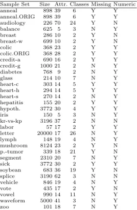
For the purpose of our study, we used 33 well-recognized sample sets from many domains recommended by Weka [9]. There is a brief description of these sample sets in Table 1. All sample sets came from the UCI repository[1]. The prepro-cessing stages of sample sets were carried out within the Weka platform, mainly including the following three steps:
1. Applying the filter of ReplaceMissingValues in Weka to replace the missing values of attributes.
2. Applying the filter of Discretize in Weka to discretize numeric attributes. Therefore, all the attributes are treated as nominal.
3. It is well known that, if the number of values of an attribute is almost equal to the number of samples in a sample set, this attribute does not contribute any information to classification. So we used the filter of Remove in Weka to delete these attributes. Three occurred within the 33 sample sets, namely Hospital Number in sample set horse-colic.ORIG, Instance Name in sample set Splice and Animal in sample set zoo.
To avoid the zero-frequency problem, we used the Laplace estimation. More precisely, assuming that there are nc samples that have the class label as c, t total samples, and k class values in a sample set. The frequency-based probabil-ity estimation calculates the estimated probabilprobabil-ity by p(c) = nc
t. The Laplace estimation calculates it as p(c) = nc+1
t+k . In the Laplace estimation, p(ai|c) is calculated by p(ai|c) = nnic+1
c+vi, where vi is the number of values of attribute Ai
and nicis the number of samples in class c with Ai= ai.
In our experiments, two groups of comparisons have been performed. We compared CLLTree with na¨ıve Bayesian related algorithms, such as NBTree, NB, TAN; and with PETs variant algorithms, such as C4.4 ,C4.4-B(C4.4 with bag-ging), C4.5-L(C4.5 with Laplace estimation) and C4.5-B(C4.5 with bagging). We implemented CLLTree within the Weka framework [9], and used the implemen-tation of other learning algorithms in Weka. In all experiments, the experimental result for each algorithm was measured via a ten-fold cross validation. Runs with various algorithms were carried out on the same training sets and evaluated on the same test sets. In particular, the cross-validation folds were the same for all the experiments on each sample set. Finally, we conducted two-tailed t-test with a significantly different probability of 0.95 to compare our algorithm with others. That is, we speak of two results for a sample set as being “significantly different” only if the difference is statistically significant at the 0.05 level according to the corrected two-tailed t-test [6].
Table 2 and 4 show the experimental results in terms of CLL and AUC. The corresponding summaries of t-test results are demonstrated in Table 3 and
Table 1. Description of sample sets used by the experiments.
Sample Set Size Attr. Classes Missing Numeric anneal 898 39 6 Y Y anneal.ORIG 898 39 6 Y Y audiology 226 70 24 Y N balance 625 5 3 N Y breast 286 10 2 Y N breast-w 699 10 2 Y N colic 368 23 2 Y Y colic.ORIG 368 28 2 Y Y credit-a 690 16 2 Y Y credit-g 1000 21 2 N Y diabetes 768 9 2 N Y glass 214 10 7 N Y heart-c 303 14 5 Y Y heart-h 294 14 5 Y Y heart-s 270 14 2 N Y hepatitis 155 20 2 Y Y hypoth. 3772 30 4 Y Y iris 150 5 3 N Y kr-vs-kp 3196 37 2 N N labor 57 17 2 Y Y letter 20000 17 26 N Y lymph 148 19 4 N Y mushroom 8124 23 2 Y N p.-tumor 339 18 21 Y N segment 2310 20 7 N Y sick 3772 30 2 Y Y soybean 683 36 19 Y N splice 3190 62 3 N N vehicle 846 19 4 N Y vote 435 17 2 Y N vowel 990 14 11 N Y waveform 5000 41 3 N Y zoo 101 18 7 N Y
5. Multi-class AUC has been calculated by M-measure[4] in our experiments. Table 6 and 7 display the ACC comparison and t-test results respectively. In all t-test tables, entry w/t/l means that the algorithm in the corresponding row wins in w sample sets, ties in t sample sets, and loses in l sample sets. Our observations are summarized as follows.
1. CLLTree outperforms NBTree in terms of CLL and AUC significantly, and slightly better in ACC. The results in CLL (Table 3) show that CLLTree wins in 10 sample sets, ties in 23 sample sets and loses in 0 sample sets. In AUC (Table 5), CLLTree wins in 5 sample sets, ties in 27 sample sets and loses only in one. Additionally, CLLTree surpasses NBTree in the ACC performance as well. It wins in 3 sample sets and loses in 1 sample set. 2. CLLTree is the best among the rest of learning algorithms in AUC.
Com-pared with C4.4, it wins in 19 sample sets, ties in 14 sample sets and loses in 0 sample sets. Since C4.4 is the state-of-art decision tree algorithm designed specifically for yielding accurate ranking, this comparison also provides evi-dence to support CLLTree. Compared with na¨ıve Bayes, our algorithm also wins in 9 sample sets, ties in 21 sample sets and loses in 3 sample sets.
3. In terms of the average classification accuracy (Table 6), CLLTree achieves the highest ACC among all algorithms. Compared with na¨ıve Bayes, it wins in 11 sample sets, ties in 21 sample sets and loses in 1 sample set. The average ACC for na¨ıve Bayes is 82.82%, lower than that of CLLTree. Furthermore, CLLTree also outperforms TAN significantly. It wins 6 sample sets, ties in 24 sample sets and loses in 3 sample sets. The average ACC for TAN is 84.64%, which is lower than our algorithm as well. And last, CLLTree is also better than C4.5, the implementation of traditional decision trees, in 8 sample sets. 4. Although C4.4 outperforms CLLTree in CLL, our algorithm is definitely better than C4.4 in the overall performance. C4.4 sacrifices its tree size to improve probability estimation, which could produce the “overfitting” problem and will be noise sensitive. Therefore, in a practical perspective, CLLTree is more suitable for many real applications.
5
Conclusion
In this paper, we have proposed a novel algorithm CLLTree to improve prob-ability estimation in NBTree. The empirical results prove our expectation that CLL and AUC are significantly improved and ACC is slightly better compared to other classic learning algorithms. There is still room to improve probability estimation. For example, after the structure is learned, we can use parameter learning algorithms to tune the conditional probability estimates on the path attributes. And we can find the right tree size for our model, i.e. possibly using model-selection criteria to decide when to stop the splitting.
References
1. C. Blake and C.J. Merz. Uci repository of machine learning database.
2. Charles Elkan. The foundations of cost-sensitive learning. In Proceedings of the Seventeenth International Joint Conference on Artificial Intelligence, 1991. 3. N. Friedman, D. Geiger, and M. Goldszmidt. Bayesian network classifiers. Machine
Learning, 29, 1997.
4. D. J. Hand and R. J. Till. A simple generalisation of the area under the roc curve for multiple class classification problems. Machine Learning, 45, 2001.
5. Ron Kohavi. Scaling up the accuracy of naive-bayes classifiers: a decision-tree hybrid. In Proceedings of the Second International Conference on Knowledge Dis-covery and Data Mining, 1996.
6. C. Nadeau and Y. Bengio. Inference for the generalization error. Machine Learning, 52(40), 2003.
7. J. Pearl. Probabilistic Reasoning in Intelligent Systems. Morgan Kaufmann, 1988. 8. F. J. Provost and P. Domingos. Tree induction for probability-based ranking.
Machine Learning, 52(30), 2003.
9. I. H. Witten and E. Frank. Data Mining –Practical Machine Learning Tools and Techniques with Java Implementation. Morgan Kaufmann, 2000.
10. H. Zhang and J. Su. Conditional independence trees. In Proceedings of the 15th European Conference on Machine Learning (ECML2004). Springer, 2004.
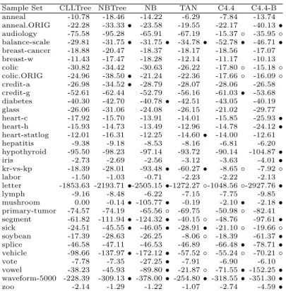
Table 2.Experimental results for CLLTree versus Na¨ıve Bayes Tree (NBTree), na¨ıve Bayes (NB) and Tree Augmented Na¨ıve Bayes (TAN); C4.4, C4.4 with bagging (C4.4-B) and C4.5 with Laplace estimation (C4.5-L): Conditional Log Likelihood (CLL) & standard deviation.
Sample Set CLLTree NBTree NB TAN C4.4 C4.4-B anneal -10.78 -18.46 -14.22 -6.29 -7.84 -13.74 anneal.ORIG -22.28 -33.33 • -23.58 -19.55 -22.17 -40.13 • audiology -75.58 -95.28 -65.91 -67.19 -15.37 ◦ -35.95 ◦ balance-scale -29.81 -31.75 • -31.75 • -34.78 • -52.78 • -46.71 • breast-cancer -18.88 -20.47 -18.37 -18.17 -18.56 -17.07 breast-w -11.43 -17.47 -18.28 -12.14 -11.17 -10.13 colic -30.82 -34.42 -30.63 -26.22 -17.80 ◦ -15.18 ◦ colic.ORIG -24.96 -38.50 • -21.24 -22.36 -17.66 ◦ -16.09 ◦ credit-a -26.98 -34.52 • -28.79 -28.07 -28.06 -26.58 credit-g -52.61 -62.44 -52.79 -56.16 -61.03 • -53.68 diabetes -40.30 -42.70 -40.78 • -42.51 -43.05 -40.19 glass -26.06 -31.06 -24.08 -26.15 -21.02 -29.77 heart-c -17.92 -15.70 -13.91 -14.01 -15.85 -25.93 • heart-h -15.93 -14.73 -13.49 -12.96 -14.78 -24.12 • heart-statlog -12.01 -16.31 -12.25 -14.60 • -14.00 -12.61 hepatitis -9.38 -9.18 -8.53 -8.16 -6.81 -6.20 hypothyroid -95.50 -98.23 -97.14 -93.72 -90.14 -104.87 • iris -2.73 -2.69 -2.56 -3.12 -3.63 -4.01 • kr-vs-kp -18.39 -28.01 -93.48 • -60.27 • -8.65 ◦ -7.92 ◦ labor -1.50 -1.03 -0.71 -2.23 -2.22 -2.13 letter -1853.63 -2193.71 •-2505.15 •-1272.27 ◦-1048.56 ◦-2927.76 • lymph -9.16 -8.48 -6.22 -7.15 -7.75 -9.85 mushroom 0.00 -0.14 • -105.77 • -0.19 -2.10 • -2.18 • primary-tumor -74.57 -74.19 -65.56 ◦ -69.75 -50.98 ◦ -82.41 segment -61.82 -111.94 • -124.32 • -40.15 ◦ -48.76 -97.61 • sick -24.51 -45.55 • -46.05 • -28.91 • -21.10 ◦ -19.66 ◦ soybean -17.39 -28.63 -26.25 -8.06 ◦ -18.39 -61.37 • splice -46.58 -47.11 -46.53 -46.89 -66.48 • -78.71 • vehicle -98.66 -137.97 • -172.12 • -57.52 ◦ -55.24 ◦ -70.21 ◦ vote -7.78 -7.35 -27.25 • -7.91 -6.90 -6.10 vowel -38.23 -45.93 -89.80 • -21.87 ◦ -71.55 • -152.25 • waveform-5000 -228.39 -309.13 • -378.00 • -254.80 • -318.55 • -351.30 • zoo -2.14 -1.29 -1.22 -1.07 -2.74 -4.59 • •, ◦ statistically significant degradation or improvement compared with CLLTree
Table 3.Summary on t-test of experimental results: CLL comparisons on CLL-Tree, NBCLL-Tree, NB, TAN, C4.4 and C4.4-B. An entry w/t/l means that the algo-rithm at the corresponding row wins in w sample sets, ties in t sample sets, and loses in l sample sets, compared to the algorithm at the corresponding column.
C4.4-B C4.4 TAN NB NBTree C4.4 19/7/7 TAN 16/12/5 8/17/8 NB 14/9/10 5/14/14 3/18/12 NBTree 10/15/8 5/16/12 2/20/11 7/22/4 CLLTree 14/13/6 6/19/8 5/23/5 11/21/1 10/23/0
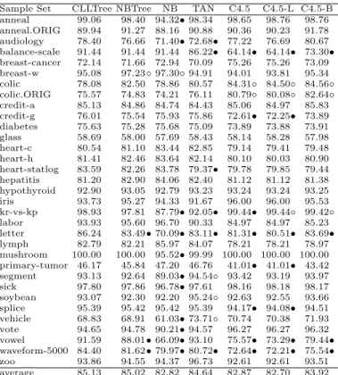
Table 4.Experimental results for CLLTree versus Na¨ıve Bayes Tree (NBTree), na¨ıve Bayes (NB) and Tree Augmented Na¨ıve Bayes (TAN); C4.4 and C4.4 with bagging (C4.4-B): Area Under the Curve (AUC) & standard deviation.
Sample Set CLLTree NBTree NB TAN C4.4 C4.4-B anneal 95.97 96.31 96.18 96.59 93.67 94.48 anneal.ORIG 93.73 93.55 94.50 95.26 91.01 • 93.21 audiology 70.36 70.17 70.02 70.25 64.04 • 69.05 • balance-scale 84.69 84.64 84.64 78.34 • 61.40 • 66.55 • breast-cancer 68.00 67.98 70.18 66.18 60.53 • 64.55 breast-w 98.64 99.25◦ 99.25 ◦ 98.72 98.22 98.83 colic 82.08 86.78 84.36 85.04 83.96 88.20 ◦ colic.ORIG 81.95 79.83 81.18 81.93 83.00 85.98 credit-a 92.06 91.34 91.86 91.35 89.59 • 90.53 • credit-g 79.14 77.53 79.10 77.92 70.07 • 74.21 • diabetes 82.57 82.11 82.61 81.33 76.20 • 79.10 • glass 82.17 79.13 78.42 • 78.32 • 80.11 80.30 heart-c 83.89 84.00 84.11 84.03 83.27 • 83.65 heart-h 83.87 83.90 84.00 83.88 83.30 • 83.64 heart-statlog 91.34 89.83 91.34 88.19 • 82.81 • 86.51 • hepatitis 83.48 85.69 89.36 86.06 79.50 82.43 hypothyroid 88.23 87.66 88.10 87.84 80.62 • 81.44 • iris 98.72 98.85 98.99 98.49 98.67 98.77 kr-vs-kp 99.82 99.44 95.19 • 98.06 • 99.93 99.97 ◦ labor 95.29 96.63 98.67 93.75 87.17 90.79 letter 99.36 98.51• 96.91 • 99.12 • 95.52 • 98.41 • lymph 89.12 88.94 90.25 89.16 86.30 88.17 mushroom 100.00 100.00 99.80 •100.00 100.00 100.00 primary-tumor 75.33 74.71 75.58 75.43 68.53 • 73.05 • segment 99.40 99.11• 98.35 • 99.63 ◦ 99.08 • 99.49 sick 98.44 94.46• 95.87 • 98.31 99.03 99.23 soybean 99.81 99.72 99.79 99.87 98.02 • 98.95 • splice 99.45 99.44 99.46 ◦ 99.40 98.06 • 98.74 • vehicle 86.68 85.86 80.58 • 91.14 ◦ 85.96 89.02 ◦ vote 98.50 98.61 97.15 • 98.78 97.43 98.31 vowel 99.35 98.59• 95.98 • 99.64 91.574 • 96.44 • waveform-5000 94.74 93.71• 95.32 ◦ 93.87 • 81.36 • 90.04 • zoo 88.64 89.02 88.88 88.93 80.26 • 80.88 • average 89.83 89.55 89.58 89.54 85.70 87.97
•, ◦ statistically significant degradation or improvement compared with CLLTree
Table 5.Summary on t-test of experimental results: AUC comparisons on CLL-Tree, NBCLL-Tree, NB, TAN, C4.4 and C4.4-B.
C4.4-B C4.4 TAN NB NBTree C4.4 0/15/18 TAN 12/19/2 18/13/2 NB 14/12/7 21/7/5 4/20/9 NBTree 8/20/5 19/12/2 3/25/5 7/25/1 CLLTree 14/16/3 19/14/0 6/25/2 9/21/3 5/27/1
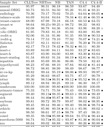
Table 6.Experimental results for CLLTree versus Na¨ıve Bayes Tree (NBTree), na¨ıve Bayes (NB) and Tree Augmented Na¨ıve Bayes (TAN); C4.5, C4.5 with Laplace estimation (C4.5-L), and C4.5 with bagging (C4.5-B): Classification Accuracy (ACC) & standard deviation.
Sample Set CLLTree NBTree NB TAN C4.5 C4.5-L C4.5-B anneal 99.06 98.40 94.32• 98.34 98.65 98.76 98.76 anneal.ORIG 89.94 91.27 88.16 90.88 90.36 90.23 91.78 audiology 78.40 76.66 71.40• 72.68• 77.22 76.69 80.67 balance-scale 91.44 91.44 91.44 86.22• 64.14• 64.14• 73.30• breast-cancer 72.14 71.66 72.94 70.09 75.26 75.26 73.09 breast-w 95.08 97.23◦ 97.30◦ 94.91 94.01 93.81 95.34 colic 78.08 82.50 78.86 80.57 84.31◦ 84.50◦ 84.56◦ colic.ORIG 75.57 74.83 74.21 76.11 80.79◦ 80.08◦ 82.64◦ credit-a 85.13 84.86 84.74 84.43 85.06 84.97 85.83 credit-g 76.01 75.54 75.93 75.86 72.61• 72.25• 73.89 diabetes 75.63 75.28 75.68 75.09 73.89 73.88 73.91 glass 58.69 58.00 57.69 58.43 58.14 58.28 57.98 heart-c 80.54 81.10 83.44 82.85 79.14 79.41 79.48 heart-h 81.41 82.46 83.64 82.14 80.10 80.03 80.90 heart-statlog 83.59 82.26 83.78 79.37• 79.78 79.85 79.44 hepatitis 81.20 82.90 84.06 82.40 81.12 81.12 81.38 hypothyroid 92.90 93.05 92.79 93.23 93.24 93.24 93.25 iris 93.73 95.27 94.33 91.67 96.00 96.00 95.53 kr-vs-kp 98.93 97.81 87.79• 92.05• 99.44• 99.44◦ 99.42◦ labor 93.93 95.60 96.70 90.33 84.97 84.97 85.23 letter 86.24 83.49• 70.09• 83.11• 81.31• 80.51• 83.69• lymph 82.79 82.21 85.97 84.07 78.21 78.21 78.97 mushroom 100.00 100.00 95.52• 99.99 100.00 100.00 100.00 primary-tumor 46.17 45.84 47.20 46.76 41.01• 41.01• 43.42 segment 93.13 92.64 89.03• 94.54◦ 93.42 93.19 93.97 sick 97.80 97.86 96.78• 97.61 98.16 98.18 98.17 soybean 93.07 92.30 92.20 95.24◦ 92.63 92.55 93.66 splice 95.39 95.42 95.42 95.39 94.17• 94.08• 94.51 vehicle 68.83 68.91 61.03• 73.71◦ 70.74 70.38 71.93 vote 94.65 94.78 90.21• 94.57 96.27 96.27 96.32 vowel 91.59 88.01• 66.09• 93.10 75.57• 73.29• 79.44• waveform-5000 84.40 81.62• 79.97• 80.72• 72.64• 72.21• 75.54• zoo 93.86 94.55 94.37 96.73 92.61 92.61 93.51 average 85.13 85.02 82.82 84.64 82.87 82.70 83.92 •, ◦ statistically significant degradation or improvement compared with CLLTree
Table 7.Summary on t-test of experimental results: ACC comparisons on CLL-Tree, NBCLL-Tree,NB, TAN, C4.5, C4.5-L and C4.5-B.
C4.5 C4.5-L C4.5-B TAN NB NBTree C4.5-L 3/30/0 C4.5-B 6/27/0 7/26/0 TAN 8/22/3 10/19/4 3/25/5 NB 8/13/12 8/14/11 5/15/13 3/19/11 NBTree 7/24/2 8/24/1 5/25/3 3/26/4 11/22/0 CLLTree 8/23/2 7/23/3 4/26/3 6/24/3 11/21/1 3/29/1