CERN-EP-2018-337 17 December 2018
c
2018 CERN for the benefit of the ALICE Collaboration.
Reproduction of this article or parts of it is allowed as specified in the CC-BY-4.0 license.
Real-time data processing in the ALICE High Level Trigger at the LHC
ALICE Collaboration∗
Abstract
At the Large Hadron Collider at CERN in Geneva, Switzerland, atomic nuclei are collided at ultra-relativistic energies. Many final-state particles are produced in each collision and their properties are measured by the ALICE detector. The detector signals induced by the produced particles are digitized leading to data rates that are in excess of 48 GB/s. The ALICE High Level Trigger (HLT) system pioneered the use of FPGA- and GPU-based algorithms to reconstruct charged-particle trajectories and reduce the data size in real time. The results of the reconstruction of the collision events, available online, are used for high level data quality and detector-performance monitoring and real-time time-dependent detector calibration. The online data compression techniques developed and used in the ALICE HLT have more than quadrupled the amount of data that can be stored for offline event processing.
∗See Appendix A for the list of collaboration members
Outline of this article
In the following, after introducing the ALICE (A Large Ion Collider Experiment) apparatus and high-lighting specific detector subsystems relevant to this article, the ALICE High Level Trigger (HLT) archi-tecture and the system software that operates the compute cluster are presented. Thereafter, the custom Field Programmable Gate Array (FPGA) based readout card, which is employed to receive data from the detectors, is described. An overview of the most important processing components employed in the HLT follows. The updates made to the HLT for LHC Run 2, that provided the capability to operate at twice the event rate compared to LHC Run 1, are discussed. The track and event reconstruction methods used, along with the quality of their performance are highlighted. The presentation of the ALICE HLT is concluded with an analysis of the maximum feasible data and event rates, along with an outlook in particular to LHC Run 3.
1 The ALICE detector
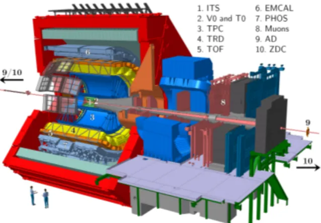
Figure 1: The ALICE detector system at the LHC.
The ALICE apparatus [1] comprises various detector systems (Fig. 1), each with its own specific technol-ogy choice and design, driven by the physics requirements and the experimental conditions at the LHC [2]. The most stringent design constraint is the extreme charged particle multiplicity density (dNch/dη) in heavy-ion collisions, which was measured at midrapidity to be 1943 ± 54 in the 5% most central (head-on) Pb–Pb events at√sNN = 5.02 TeV [3]. The main part of the apparatus is housed in a solenoidal magnet, which generates a field of 0.5 T within a volume of 1600 m3. The central barrel of ALICE is composed of various detectors for tracking and particle identification at midrapidity. The main tracking device is the Time Projection Chamber (TPC) [4]. In addition to tracking, it provides particle identifi-cation information via the measurement of the specific ionization energy loss (dE/dx). The momentum and angular resolution provided by the TPC is further enhanced by using the information from the six layer high-precision silicon Inner Tracking System (ITS) [5], which surrounds the beam pipe. Outside the TPC there are two large particle identification detectors: the Transition Radiation Detector (TRD) [6] and the Time-Of-Flight (TOF) [7]. The central barrel of ALICE is augmented by dedicated detectors that are used to measure the energy of photons and electrons, the Photon Spectrometer (PHOS) [8] and ElectroMagnetic Calorimeter (EMCal) [9]. In the forward direction of one of the particle beams is the muon spectrometer [10], with its own large dipole magnet. In addition, there are other fast-interaction detectors including the V0, T0 [11], and Zero Degree Calorimeter (ZDC) [12]. As the TPC is the most relevant for the performance of the HLT a more detailed description of it follows.
The TPC is a large cylindrical, gas-filled drift detector with two readout planes at its end-caps. A central high voltage membrane provides the electric drift field and divides the total active volume of 85 m3into two halves. Each charged particle traversing the gas in the detector volume produces a trace of ionization
along its own trajectory. The ionization electrons drift towards the readout planes, which are subdivided into 18 trapezoidal readout sectors. The readout sectors are segmented into 15488 readout pads each, arranged in 159 consecutive rows in radial direction. Upon their arrival at the readout planes, ionization electrons induce electric signals on the readout pads. For an issued readout trigger, the signals are digitized by a 10 bit ADC at a frequency of 10 MHz, sampling the maximum drift time of about 100 µs into 1000 time bins. This results in a total of 5.5 · 108ADC samples containing the full digitized TPC pulse height information. The size of data corresponding to a single collision event is about 700 MB. A zero-suppression algorithm implemented in an ASIC reduces the proton-proton TPC event size to typically 100 kB. The exact event size depends on the background, trigger setting, and interaction rate. Central Pb–Pb collisions produce up to 100 MB of TPC data, which can grow up to around 200 MB with pile-up. The TPC is responsible for the bulk of the data rate in ALICE. In Run 2, when operated at event rates of up to 2 kHz (pp and p–Pb) and 1 kHz (Pb–Pb), it reads out up to 40 GB/s. In addition, the total readout rate has a contributixon of a few GB/s from other ALICE detectors, some of them operating at trigger rates up to 3.5 kHz. The volume of data taken at these rates exceeds the capacity for permanent storage considerably.
The amount of data that is stored can be reduced in a number of ways. The most widely used methods are compression of raw data (using either lossless or lossy schemes) and online selection of a subset of physically interesting events (triggering), which discards a certain fraction of the data read out by the detector [13–15]. A hierarchical trigger system performs this type of selection by having the lower hardware levels base their decision only on a subset of the data recorded by trigger detectors. The highest trigger level is the software-based High Level Trigger (HLT), which has access to the entire detector data set.
2 The High Level Trigger (HLT)
2.1 From LHC Run 1 commissioning to LHC Run 2 upgrades
A first step in transforming raw data to fully reconstructed physics information in real time was achieved with the beginning of LHC Run 1 on November 23rd, 2009, when protons collided in the center of the ALICE detector for the first time. On the morning of December 6th, stable beams at an energy of 450 GeV per beam were delivered by the LHC for the first time, and the HLT reconstructed the first charged-particle tracks from pp collisions by processing data from all available ALICE detectors. Though the HLT was designed as trigger and was operated as such at the start of Run 1, the collaboration found that by using it for data compression one could record all data to storage, thus optimizing the use of beam time. This was possible due to the the quality of the online reconstruction and the increased bandwidth to storage. Throughout Run 1 the HLT was successful as an online reconstruction and data compression facility.
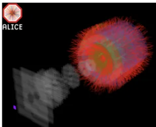
After the LHC Run 1, that lasted to the beginning of 2013, parts of the ALICE detector were upgraded for LHC Run 2, which started in 2015. The most important change was the upgrade of the TPC readout electronics, employing a new version of the Readout Control Unit (RCU2) [16] which uses the updated optical link speed of 3.125 Gbps instead of the previous readout rate of 2.125 Gbps. The upgrades, along with an improved TPC readout scheme, doubled the theoretical maximum TPC readout data rate to 48 GB/s, thus allowing ALICE to record twice as many events. In addition, the HLT farm underwent a consolidation phase during that period in order to be able to cope with the increased data rate of Run 2. This update improved several parts of the HLT based on the experience from Run 1. While the HLT processed up to 13 GB/s of TPC data in Run 1 [17], the new HLT infrastructure allows for the processing of the full 48 GB/s (see Section 4). Figure 2 shows a screenshot of the online event display during a Run 2 heavy-ion run1 with active GPU-accelerated online tracking in the HLT, of which will be described in
Figure 2: Visualization of a heavy-ion collision recorded in ALICE with tracks reconstructed in real time on the GPUs of the HLT.
the following.
2.2 General description
The main objective of the ALICE HLT is to reduce the data volume that is stored permanently to a reasonable size, so to fit in the allocated tape space. The baseline for the entire HLT operation is full real-time event reconstruction. This is required for more elaborate compression algorithms that use re-constructed event properties. In addition, the HLT enables a direct high-level online Quality Assurance (QA) of the data received from the detectors, which can immediately reveal problems that arise during data taking. Several of the ALICE sub-detectors (like the TPC) are so called drift-detectors that are sensitive to environmental conditions like ambient temperature and pressure. Thus a precise event recon-struction requires detector calibration, which in turn requires results from a first reconrecon-struction as input. It is natural then to perform as much calibration as possible online in the HLT, which is also immediately available for offline event reconstruction, and thus reduces the required offline compute resources. In summary, the HLT tasks are online reconstruction, calibration, quality monitoring and data compression. The HLT is a compute farm composed of 180 worker nodes and 8 infrastructure nodes. It receives an exact copy of all the data from the detector links. After processing the data, the HLT sends its reconstruction output to the Data Acquisition (DAQ) via dedicated optical output links. Output channels to other systems for QA histograms, calibration objects, etc., are described later in this paper. In addition the HLT sends a trigger decision. The decision contains a readout list, which specifies the output links that are to be stored and are to be discarded by DAQ. A collision event is fully accepted if all detector links are allowed to store data and rejected if the decision is negative for all links. Data on some links may be replaced by issuing a negative decision for those links and injecting (reconstructed) HLT data instead. DAQ buffers all the event fragments locally and waits for the readout decision from the HLT, which has an average delay of 2–4 seconds for Pb–Pb data, while in rare cases the maximum delay reaches 10 seconds. Then, DAQ builds the events using only the fraction of the links accepted by the HLT plus the HLT payloads and moves the events first to temporary storage and later to permanent storage. Figure 3 illustrates how the HLT is integrated in the ALICE data readout scheme.
The compute nodes use off-the-shelf components except for the Read Out Receiver Card (RORC - out-lined in Section 2.3), which is a custom FPGA-based card developed for Run 1 and Run 2. During LHC Run 1 the HLT farm consisted of 248 servers including 117 dedicated Front-End Processor (FEP) nodes equipped with RORCs for receiving data from the detectors and sending data to DAQ. The re-maining servers were standard compute nodes with two processors each, employing AMD Magny-Cours twelve-core CPUs and Intel Nehalem Quad-core CPUs. A subset of 64 compute nodes was equipped
TPC ITS TRD TOF EMCAL PHOS MUON HMPID CPV FMD PMD V0 T0 AD ZDC Acorde
Splitters Detectors
216 links 60 links 18 links 72 links 40 links 15 links 22 links 14 links 1 link 1 link 6 links 1 link 1 link 1 link 1 link 1 link
3.125 GBit 2.125 GBit 4.0 GBit 2.125 GBit 2.125 GBit 2.125 GBit 2.125 GBit 2.125 GBit 2.125 GBit 2.125 GBit 2.125 GBit 2.125 GBit 2.125 GBit 2.125 GBit 2.125 GBit 2.125 GBit
66 HLT Input Nodes (FEP)
180 HLT
worker nodes
(172 compute
nodes)
High Level
T
rigger (HL
T)
Data
Acquisition (DAQ)
28 HLTOUT links 5.3125 GBit LDCs GDCs Event merging, round-robin processing using all nodes including FEP and HLTOUTTo permanent storage 8 HLT Output Nodes (HLTOUT)
To online QA
Figure 3: The ALICE HLT in the data readout scheme during Run 2. In the DAQ system the data flow through the local and the global data concentrators, LDC and GDC, respectively. In parallel, HLT ships QA and calibration data via dedicated interfaces.
with NVIDIA Fermi GPUs as hardware accelerators for track reconstruction, described in Section 3.3. In addition, there were around 20 infrastructure nodes for provisioning, storage, database service and monitoring. Two independent networks connected the cluster: a gigabit Ethernet network for manage-ment and a fast fat-tree InfiniBand QDR 40 GBit network for data processing. Remote managemanage-ment of the compute nodes was realized via the custom developed FPGA-based CHARM card [18] that emulates and forwards a VGA interface, as well as the BMC (Board Management Controller) iKVM (Keyboard, Video, Mouse over IP) available as IPMI (Intelligent Platform Management Interface) standard in new compute nodes [19].
In 2014, a new HLT cluster was installed for Run 2 replacing the older servers, in particular the Run 1 FEP nodes, which were operational since 2008, during system commissioning. The availability of mod-ern hardware, specifically the faster PCI Express interface and network interconnect, allowed for a con-solidation of the different server types. The Run 2 HLT employs 188 ASUS ESC4000 G2S servers with two twelve-core Intel Xeon IvyBridge E5-2697 CPUs running at 2.7 GHz and one AMD S9000 GPU each. In order to exclude possible compatibility problems before purchase, a full HLT processing chain was stress tested on the SANAM [20] compute cluster at the GSI Helmholtz Centre for Heavy-Ion Re-search using almost identical hardware. The front-end and output functionality was integrated into 66 input nodes and 8 output nodes, where the input nodes serve also as compute nodes. They were equipped with RORCs for input and output allowing for a better overall resource utilization of the processors, while the infrastructure nodes of the same server type were kept separate. This reduction in the total number of servers also reduced the required rack-space and number of network switches and cables. Furthermore, the fast network was upgraded to 56 GBit FDR InfiniBand. Table 1 gives an overview of the Run 1 and Run 2 computing farms.
Considering the requirement of high reliability, which is driven among other things by the operating cost of the LHC, a fundamental design criterion is the robustness of the overall system with regard to
Table 1: Overview of the HLT Run 1 and Run 2 production clusters.
Run 1 farm Run 2 farm
CPU cores Opteron / Xeon Xeon E5-2697
2784 cores, up to 2.27 GHz 4480 cores, 2.7 GHz
GPUs 64 × GeForce GTX480 180 × FirePro S9000
Total memory 6.1 TB 23.1 TB
Total nodes 248 188
Infrastructure nodes 22 8
Worker nodes 226 180
Compute nodes (CN) 95 172
Input nodes 117 (subset of CNs)66
Output nodes 14 8
Bandwidth to DAQ 5 GB/s 12 GB/s
Max. input bandwidth 25 GB/s 48 GB/s
Detector links 452 473
Output links 28 28
RORC type H-RORC C-RORC
Host interface PCI-X PCI-Express
Max. PCI bandwidth 940 MB/s 3.6 GB/s
Optical links 2 12
Max. link bandwidth 2.125 Gbps 5.3125 Gbps
Clock frequency 133.3 MHz 312.5 MHz
On-board memory 128 MB up to 16 GB
component failure. Therefore, all the infrastructure nodes are duplicated in a cold-failover configuration. The workload is distributed in a round-robin fashion among all compute nodes, so that if one pure compute node fails it can easily be excluded from the data-taking period. Potentially the failover requires a reboot and a restart of the ALICE data taking. This scenario only takes a few minutes, which is acceptable given the low failure rate of the system; for instance, there were only 9 node failures in 1409 hours of operation during 2016. A more severe problem would be the failure of an input node, because in that case the HLT is unable to receive data from several optical links. Even though there are spare servers and spare RORCs, manual intervention is needed to reconnect the fibers if the FEP node cannot be switched on remotely. However, this scenario occurred only twice in all the years of HLT operation (from 2009 to 2017). Since the start of Run 2, the entire production cluster is connected to an online uninterruptible power supply.
Since the installation of the Run 2 compute farm, parts of the former compute infrastructure are reused as a development cluster, to allow for software development and realistic scale testing without disrupting the data taking activities. Additionally, the development cluster is used as an opportunistic GRID com-pute resource (see Section 2.5) and an integration cluster for the ALICE Online-Offline (O2) computing upgrade foreseen for Run 3 [21]. The O2project includes upgrades to the ALICE computing model, a software framework that integrates the online and offline data processing, and the construction of a new computing facility.
2.3 The Common Read-Out Receiver Card
The Read-Out Receiver Card (RORC) is the main input and output interface of the HLT for detector data. It is an FPGA-based server plug-in board that connects the optical detector links to the HLT cluster and serves as the first data processing stage. During Run 1 this functionality was provided by the HLT-dedicated RORC (H-RORC) [22], a PCI-X based FPGA board that connects to up to two optical detector links at 2.125 Gbps. The need for higher link rates, the lack of the PCI-X interface on recent server PCs, as well as the limited processing capabilities of the H-RORC with respect to the Run 2 data rates required a new RORC for Run 2. None of the commercially available boards were able to provide the required
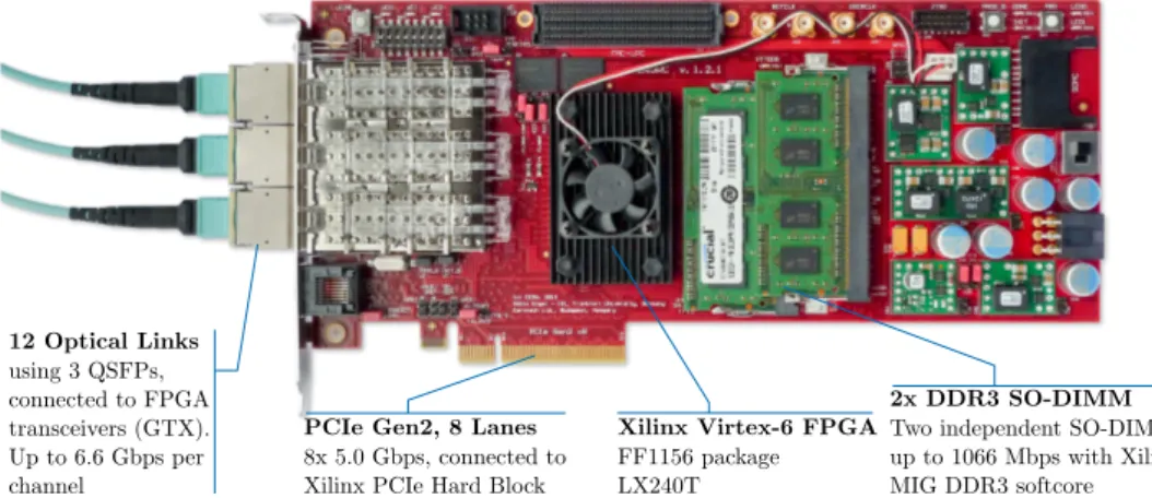
functionality, which led to the development of the Common Read-Out Receiver Card (C-RORC) as a custom readout board for Run 2. The hardware was developed in order to enable the readout of detec-tors at higher link speeds, extend the hardware-based online processing of detector data, and provide state-of-the-art interfaces with a common hardware platform. Additionally, technological advancements enabled a factor six higher link density per board and therefore reduced the number of boards required for the same amount of optical links compared to the previous generation of RORCs. One HLT C-RORC receives up to 12 links. A photograph of the board is shown in Fig. 4. The C-RORC has been part of the production systems of ALICE DAQ, ALICE HLT and ATLAS trigger and data acquisition since the start of Run 2 [23]. The FPGA handles the data stream from the links and directly writes the data into the RAM of the host machine using Direct Memory Access (DMA). A minimal kernel adapter in com-bination with a user space device driver based on the Portable Driver Architecture (PDA) [24] provides buffer management, flow control, and user-space access to the data on the host side. A custom DMA engine in the firmware enables a throughput of 3.6 GB/s from device to host. This is enough to handle the maximum input bandwidth of the TPC as the biggest data contributor (1.9 GB/s per C-RORC), the TRD as the detector with the fastest link speed (6 links at 2.3 GB/s per C-RORC), and a fully equipped C-RORC with 12 links at 2.125 Gbps (2.5 GB/s). The C-RORC FPGA implements a cluster finding al-gorithm to process the TPC raw data at an early stage. This alal-gorithm is further described in Section 3.2. The C-RORC can be equipped with several GB of on-board memory, used for data replay purposes. Generated, simulated, previously recorded, or even faulty detector data can be loaded into this on-board RAM and played back as if it were coming via the optical links. The HLT output FPGAs can be config-ured in a way to discard data right before it would be sent back to the DAQ system. The data replay can be operated independently from any other ALICE online system, detector, or LHC operational state. In combination with a configurable replay event rate, the data replay functionality provides a powerful tool to verify, scale, and benchmark the full HLT system. This feature is essential for the optimizations pre-sented in Section 4. The C-RORCs are integrated into the HLT data transport framework as data-source components for detector data input via optical links and as sink components to provide the HLT results to the DAQ system. The C-RORC FPGA firmware and its integration into the HLT is further described in [25]. The data from approximately 500 links, at link rates between 2.125 Gbps and 5.3125 Gbps, is handled via 74 C-RORCs that are installed in the HLT.
12 Optical Links using 3 QSFPs, connected to FPGA transceivers (GTX). Up to 6.6 Gbps per channel
PCIe Gen2, 8 Lanes 8x 5.0 Gbps, connected to Xilinx PCIe Hard Block
2x DDR3 SO-DIMM Two independent SO-DIMMs up to 1066 Mbps with Xilinx MIG DDR3 softcore Xilinx Virtex-6 FPGA
FF1156 package LX240T
Figure 4: The Common Read-Out Receiver Card.
2.4 Cluster commissioning, software deployment, and monitoring
The central goal for managing the HLT cluster is automation that minimizes the need for manual inter-ventions and guarantees that the whole cluster is in a consistent state that can be easily controlled and modified if needed. Foreman [26] is used to automatize the basic installation of the servers via PXE-boot. The operating system (OS) that is currently used on all of the servers is CERN CentOS 7. Once the OS
is installed on these servers, Puppet [27] controls and applies the desired configuration to each server. Puppet efficiently integrates into Foreman and allows for servers to be organized into groups according to different roles and apply changes to multiple servers instantaneously. With this automatized setup the complete cluster can be rebuilt, including the final configuration, in roughly three hours. For both the production and development clusters several infrastructure servers are in place, providing different ser-vices like DNS, DHCP, NFS, databases, or private network monitoring. Critical serser-vices are redundant to reduce the risk of cluster failure in case there is a problem with a single infrastructure server.
The monitoring of the HLT computing infrastructure is done using the open source tool Zabbix [28]. It allows administrators to gather metrics, be aware of the nodes health status, and react to undesired states. More than 100 metrics per node are being monitored, such as temperature, CPU load, network traffic, free disk space, disk-health status, and failure rate on the network fabric. The monitoring system autom-atizes many tasks that would require administrators’ intervention. These preemptive measures offer the possibility to replace hardware beforehand, i. e. during technical shutdowns, and to avoid failures during data taking. HLT administrators receive a daily report of the system status and, in addition, e-mail noti-fications when certain metrics exceed warning thresholds. For risky events there are automated actions in place. For instance, several shutdown procedures are performed when the node temperature reaches critical values, in order to prevent damage to the servers.
In addition to Zabbix, ALICE has developed a custom distributed log collector called InfoLogger. A parser script is employed that scans all error messages stored to the logs to find important problems in real time. These alerts can also help the detector experts with the monitoring of their systems, including automated alarms sent via e-mail or SMS.
This configuration lowers the complexity of managing a heterogeneous system with around 200 nodes for a period of at least 10 years, reducing the number of trained on-site engineers required for operation. 2.5 Alternative use cases of the HLT farm
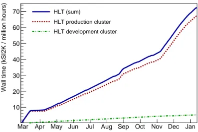
In order to maximize the usage of the servers during times when there are no collisions, a Worldwide LHC Computing Grid (WLCG) [29] configuration was developed for the cluster in cooperation with the ALICE offline team. The first WLCG setup used OpenStack [30] Virtual Machines (VM) to produce ALICE Monte Carlo (MC) simulations of particle collision events. In 2017, the WLCG setup was im-proved to use Docker [31] containers instead of OpenStack VMs, which allows for more flexibility and therefore improves efficiency with the available resources. The containers are spawned for just one job and destroyed after the job finishes. During pp data taking a part of the production cluster is contributed to the WLCG setup. During phases without data taking, like LHC year-end shutdowns and technical stops, the whole HLT production cluster is operated as a WLCG site as long as it is not needed for tests of the HLT system. Figure 5 shows the aggregated wall time of the new Docker setup from March 2017 onward. The steeper slope represents periods when the complete cluster is assigned to WLCG operation, while the plateau indicates a phase of full scale framework testing. The HLT production cluster provides a contribution to the ALICE MC simulation compute time with this opportunistic use on a best-effort basis. The WLCG setup of the HLT focuses on MC simulations because these require less storage and network resources than general ALICE Grid jobs and are thus ideally suited for opportunistic operation without side effects.
The HLT development cluster, introduced in Section 2.2, is composed of approximately 80 older servers. Not only does it allow for ongoing development of the current framework, of which runs on the produc-tion cluster, but it can also used for tests of the future framework for Run 3. During periods when no development is taking place, 60 of the nodes act as second WLCG site, in addition to the opportunistic use of the production cluster, donating the compute resources to ALICE MC jobs. To guarantee that there is no interference with data taking, the HLT development cluster is completely separated from the production environment. The development cluster is installed in different racks and also uses a different
Mar Apr May Jun Jul Aug Sep Oct Nov Dec Jan 10 20 30 40 50 60 70
Wall time (kSI2K / million hours)
HLT (sum)
HLT production cluster HLT development cluster
Figure 5: Contribution of the HLT production (dotted line) and development (double-dotted dashed line) clusters to the WLCG between March 2017 and January 2018, with the sum of both contributions shown as the solid line.
private network, which has no direct connection to the production cluster. For WLCG operation, the HLT internal networks and the network used for WLCG communication were completely separated via VLANs configured at switch level.
2.6 HLT architecture and data transport software framework
In order to transform the raw detector signals into physical properties all ALICE detectors have de-veloped reconstruction software, like TPC cluster finding (Section 3.2) and track finding (Section 3.3) algorithms. In the HLT the data processing is arranged in a pipelined data-push architecture. The re-construction process starts with local clusterization of the digitized data, continues with track finding for individual detectors, and ends with the creation of the Event Summary Data (ESD). The ESD is a complex ROOT [32] data structure that holds all of the reconstruction information for each event. In addition to the core framework described in the this section, a variety of interfaces exist to other ALICE subsystems [33]. These include the command and control interface to the Experiment Control System (ECS), the Shuttle system used for storing calibration objects for offline use, the optical links to DAQ, the online event display, and Data Quality Monitoring (DQM) for online visualization of QA histograms.
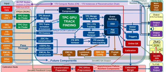
The ALICE HLT uses a modular software framework consisting of separate components, which com-municate via a standardized publisher-subscriber interface designed to cause minimal overhead for data transport [34, 35]. Such components can be data sources that feed into the HLT processing chain, either from the detector link or from other sources like TPC temperature and pressure sensors. Data sinks ex-tract data from the processing chain and send the reconstructed event and trigger decision to DAQ via the output links. Other sinks ship calibration objects or QA histograms, which are stored or visualized. In addition to source and sink components, analysis or worker components perform the main computational tasks in such a processing chain and are arranged in a pipelined hierarchy. Figure 6 gives an overview of the data flow of the most relevant components currently running in the HLT. A component reads a data set (if it is not a source), processes it, creates the output and proceeds to the next data set. Although each component processes only one event at a time, the framework pipelines the events such that thousands of events can be either in-chain in the cluster or also on a single server. Merging of event fragments, scatter-ing of events among multiple compute nodes for load balancscatter-ing, and network transfer are all handled via special processing components provided by the framework and are transparent to the worker processes.
TPC Link 1 TPC Link 216 TPC Clus-ter Finder ITS Links . . ZDC Re-construction Output Link 1 Output Link 28 Event Building Sensor Data TPC Branch Merging TPC Trans-formation (2 Instances) Input FPGA CRORC ZDC Links VZERO Links EMCAL Links
DIM from ECS
TPC GPU TRACK FINDING
TPC Merger & Track Fit
TPC / ITS Tracking ITS standa-lone tracking ESD Flat ESD VZERO Re-construction EMCAL Re-construction . . Luminous Region Prompt QA EMCAL QA TPC Clus-ter Finder
172 Compute Nodes (CN) – 172 Instances of Reconstruction Chain
Calibration Merger Calib Output TPC Offline Preprocessor Transformation Preparation ZeroMQ QA Output
ZeroMQ Feedback Loop
Output (8 HLTout Nodes) Calibration Node TPC Compression Global Trigger Other Detector Moni-toring Side Chain
Default OCDB Calibration
Pass Through
…Future Components
To FXS
1 Monitor Node
TriggersTriggersTriggers ITS SPD Vertexer Global Vertexer ITS Clusterer Asynchronous Failure-Resilient Components Transient Failure-Resilient Subscription ZMQ QA Config Calibration Online QA ZMQ ZeroMQ data mergers LHC DQM … 66 FEP Nodes (subset of CNs)
Figure 6: Schema of the HLT components. The colored boxes represent processes accelerated by GPU/FPGA (green), normal processes (blue), processes that produced HLT output that is stored (dark blue), entities that store data (purple), asynchronous failure-resilient processes (dark red), classical QA components that use the original HLT data flow (brown), input (orange), and sensor data (red). Incoming data are passed through by the C-RORC FPGA cards or processed internally. The input nodes locally merge data from all links belonging to one event. The compute nodes then merge all fragments belonging to one event and run the reconstruction. The bottom of the diagram shows the asynchronous online calibration chain with a feedback loop as described in Section 3.4.
Components situated on the same compute node pass data via a shared-memory based zero-copy scheme. With respect to Run 1 the framework underwent a revision of the interprocess-scheduling approach. The old approach, using POSIX pipes, began to cause a significant CPU load through many system calls and was consequently replaced by a shared-memory based communication.
Presently, the user simply defines the processing chain with reconstruction, monitoring, calibration, and other processing components. The user also defines the inputs for all components as well as the output at the end of the processing chain. The full chain is started automatically and distributed in the cluster. The processing configuration can be annotated with hints to guide the scheduling. In order to minimize the data transfer, the chain usually starts with local processing components on the front-end nodes (like the TPC cluster finder presented in Section 3.2). In the end, after the local steps have reduced the data volume, all required event fragments are merged on one compute node for the global event reconstruction. The data transport framework is based on three pillars. There is a primary reconstruction chain which processes all the recorded events in an event-synchronous fashion. It performs the main reconstruction and data compression tasks and is responsible for receiving and sending data. This main chain is the backbone of the HLT event reconstruction and its stability is paramount for the data taking efficiency of ALICE.
The second pillar is the data monitoring side chains, which run in parallel at low rates on the compute nodes. These subscribe transiently to the output of a component of the main chain. In this way, the side chains cannot break or stall the HLT main chain.
For Run 2 a third pillar was added, based on Zero-MQ (Zero Message Queue) message transfer [36], which provides similar features compared to the main chain but runs asynchronously. Currently, it is used for the monitoring and calibration tasks and does not merge fragments of one event but instead it is fed with fully reconstructed events from the main chain. It processes as many events as possible on a best-effort basis, skipping events when necessary. Results of the distributed components are merged periodically to combine statistics processed by each instance. The same Zero-MQ transport is also used
as an interface to DQM and as external interface which allows detector experts to query merged results of QA components running in the HLT.
The transport framework is not restricted to closed networks or computing clusters. A proof-of-principle test of the framework used locally in the HLT cluster deploys a global processing chain for a Grid-like real-time data processing. This framework was distributed on a North-South axis between Cape Town in South Africa and Tromsø in northern Norway, with Bergen (Norway), Heidelberg (Germany), and Dubna (Russia) as additional participating sites [37]. The concepts developed for the HLT are the basis for the new framework of the ALICE O2computing upgrade.
2.7 Fault tolerance and dynamic reconfiguration
Robustness of the main reconstruction chain is the most important aspect from the point of view of data taking efficiency. Therefore, the HLT was designed with several failure resiliency features. All infras-tructure services run on two redundant servers and compute node failures can be easily compensated for. Experimental and non-critical components can run in a side-chain or asynchronously via Zero-MQ, separate from the main chain.
Also the main chain itself has several fault tolerance features. Some components use code from offline reconstruction, or code written by the teams responsible for certain detector development, and hence they are not developed considering the high-reliability requirements of the HLT. Nevertheless, the HLT must still ensure stable operation in case of critical errors like segmentation faults. Thus, all components run in different processes, which are isolated from each other by the operating system. In case one component fails, the HLT framework can transparently cease the processing of that component for a short time, and then later restart the component. Although the event is still processed, the result of that particular component for this event and possibly several following events are lost. This loss of a single instance causes only a marginal loss of information.
3 Fast algorithms for fast computers
Since the TPC produces 91.1% (Pb–Pb) and 95.3% (pp) of the data volume2 and, also because of the sheer data volume, event reconstruction of the TPC data including clusterizing and tracking is the most compute intensive task of the HLT. This makes the TPC the central detector for the HLT. Its raw data are the most worthwhile target for data compression algorithms. Since a majority of the compute cycles are spent processing TPC data, it is mandatory that the TPC reconstruction code is highly efficient. It is the TPC reconstruction that leverages the compute potential of both the FPGA and GPU hardware accelera-tors in the HLT. Furthermore, since it is an ionization detector, TPC calibration is both challenging and essential.
Here, a selection of important HLT components, following the processing of the TPC data in the chain is described. The processing of the TPC data starts with the clusterization of the raw data, which happens in a streaming fashion in the FPGA while the data are received at the full optical speed. Two independent branches follow, where one component compresses the TPC clusters and replaces the TPC raw data with compressed HLT data. The second branch starts with the TPC track reconstruction using GPUs, continues with the creation of the ESD, and runs the TPC calibration and QA components.
3.1 Driving forces of information science
The design of the ALICE detector dates back two decades. At that time, the LHC computing needs could not be fulfilled based on existing technology but relied on extrapolations according to Moore’s Law [38]. Indeed the performance of computers has improved by more than three orders of magnitude
since then, but the development of microelectronics has reached physical limits in recent years. For example, processor clock rates have not increased significantly since 2004. To increase computing power various levels of parallelization are implemented, such as the use of multi- or many-core processors, or by supporting SIMD (Single Instruction, Multiple Data) vector-instructions. At this point in time computers do not become faster for single threads but they can become more powerful if parallelism is exploited. Although these developments were only partially foreseeable at the beginning of the ALICE construction phase, they have been taken into account for the realization of the HLT.
3.2 Fast FPGA cluster finder for the TPC
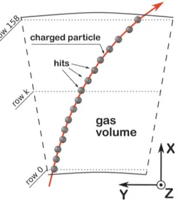
Figure 7: Schematic representation of the geometry of a TPC sector. Local y and z coordinates of a charged-particle trajectory are measured at certain x positions of 159 readout rows, providing a chain of spatial points (hits) along its trajectory.
At the beginning of the reconstruction process the so-called clusters of locally adjacent signals in the TPC have to be found. Figure 7 shows a schematic representation of a cross-section of a trapezoidal TPC sector, where the local coordinate system is such that in the middle of the sector the x-axis points away from the interaction point. One can imagine a stack of 2D pad-time planes (y-z plane in Fig. 7) in which a charged particle traversing the detector creates several neighboring signals in each 2D plane. The exact position of the intersection between the charged-particle trajectory and the 2D plane can be calculated by using the weighted mean of the signals in the plane, i. e. by determining their center of gravity. The HLT cluster-finder algorithm can be broken down into three separate steps. Firstly, the relevant signals have to be extracted from raw data and the calibration factors are applied. Next, neighboring signals and charge peaks in time-direction are identified and the center of gravity is calculated. Finally, neighboring signals in the TPC pad-row direction (x-y plane) are merged to form a cluster. These reconstructed clusters are then passed on to the subsequent reconstruction steps, such as the track finding described in Section 3.3. By design, the TPC cluster-finder algorithm is ideally suited for the implementation inside an FPGA [39], which supports small, independent and fast local memories and massively parallel computing elements. The three processing steps are mutually independent and are correspondingly implemented as a pipeline, using fast local memories as de-randomizing interfaces between these stages. In order to achieve the nec-essary pipeline throughput, each pipeline stage implements multiple custom designed arithmetic cores. The FPGA based RORCs are required as an interface of the HLT farm to the optical links. By placing the online processing of the TPC data in the FPGA, the data can be processed on-the-fly. The hardware clus-ter finder is designed to handle the data bandwidth of the optical link. Finally, a compute node receives the TPC clusters, computed in the FPGA, directly into its main memory.
An offline reference implementation of the cluster finding exists but is far too slow to be implemented online. Rather, the offline cluster finder is used as a reference for both the physics performance and the processing speed. In comparison to the hardware cluster finder executed on the FPGA, it performs additional and more complex tasks. These include checking TPC readout pads for baseline shifts and, if present, applying corrections and deconvoluting overlapping clusters using a Gaussian fit to the clus-ter shapes, which are simply split in the hardware version. Additional effects such as missing charge in the gaps between TPC sectors and malfunctioning TPC channels are considered. Finally, after the application of the drift-velocity calibration, cluster positions are transformed into the spatial x, y, and z coordinate system. In the HLT, a separate transformation component performs this spatial transformation as a later step. The evaluation in Section 3.2.1 demonstrates that the HLT hardware cluster finder delivers a performance comparable to the offline cluster finder.
Benchmarks have shown that one C-RORC with six hardware cluster finder (HardwareCF) instances is about a factor 10 faster than the offline cluster finder (OfflineCF) using 48 threads on an HLT node, as shown in Fig. 8. The software processing time measurements were done on a HLT node with dual Xeon E5-2697 CPUs for the single-threaded variant, the multi-threaded variant as well as the cluster transformation component. The single-threaded variant was also evaluated on a Core-i7 6700k CPU to show the performance improvements of using the same implementation on a newer CPU architecture. The measurements were also performed on the C-RORC.
5
10
15
20
25
30
Event Size (MB)
4 −10
3 −10
2 −10
1 −10
1
10
Processing time (s)
OfflineCF (1 thread)OfflineCF (Core-i7, 1 thread)
OfflineCF (48 threads, 24 cores)
Transformation (1 thread)
HardwareCF (1 C-RORC, 6 inst.)
Figure 8: Processing time of the hardware cluster finder and the offline cluster finder. The measurements were performed on an HLT node (circles, triangles, diamonds), a newer Core-i7 6700K CPU (squares), and on the C-RORC (inverted triangles).
Several factors increase the load on the hardware cluster finder in Run 2. The C-RORC receives more links than the former H-RORC of Run 1, with the FPGA implementing six instead of the previously two instances of the cluster finder. The TPC RCU2 sends the data at a higher rate, up to 3.125 Gbps. In addition, during 2015 and 2016, the TPC was operated with argon gas instead of neon yielding a higher gain factor, which resulted in a higher probability of noise over the zero-suppression threshold. In this situation, the cluster finder detects a larger number of clusters, though a significantly large fraction of these are fake. In addition, the readout scheme of the RCU2 was improved, disproportionately increasing
the data rate sent to the HLT compared to the link speed, yielding a net increase of a factor of 2. These modifications also required the clock frequency of the hardware cluster finder to be disproportionately scaled up compared to the link rate in order to cope with the input data rates. Major portions of the online cluster finder were adjusted, further pipelined, and partly rewritten to achieve the required clock frequency and throughput. The peak-finding step of the algorithm was replaced with an improved version more resilient to noise. This filtering reduces the number of noise induced clusters found, relaxes the load on the merging stage, and thus reduces the cluster finder output data size. The reduced output size, in combination with improvements to the software based data compression scheme, increases the overall data compression factor of the HLT (see Section 3.5).
3.2.1 Physics performance of the HLT cluster finder for the TPC
In order to reduce the amount of data stored on tape, the TPC raw data are replaced by clusters recon-structed in the HLT. The cluster-finder algorithm must be proven not to cause any significant degradation to the physical accuracy of the data. The offline track reconstruction algorithm was improved by bet-ter taking into account the slightly different behavior of the HLT clusbet-ter finder and its cenbet-ter of gravity approach compared to the offline cluster finder. The performance of the algorithm has been evaluated by looking at the charged-particle tracks reconstructed with the improved version of the offline track-reconstruction algorithm, described in Section 3.3.
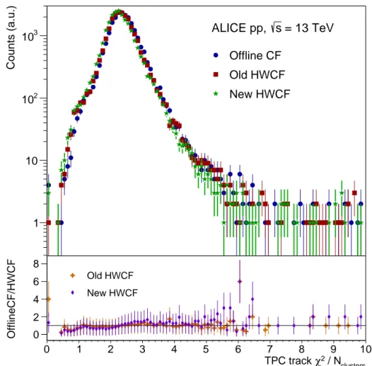
The important properties of the clusters are the spatial position, the width, and the charge deposited by the traversing particle. Figure 9 compares the χ2 distribution of TPC tracks reconstructed by the offline tracking algorithm using TPC clusters produced using either the HLT hardware cluster finder or the offline version. Since the cluster errors coming from a fit to the track are parameterized and not derived from the width of the cluster, the χ2 distribution is proportional to the average cluster-to-track residual. On a more global level, the cluster positions in the ITS are used to evaluate the track resolution of the TPC. The TPC track is propagated through the ITS volume and the probability of finding matching ITS spatial points is analyzed. Since the ITS cluster position is very precise it is a good metric for TPC track quality. However, because the occupancy for heavy-ion collisions is high, the matching requires an accurate position of the TPC track with a good transverse momentum (pT) fit for precise extrapolation. It was found that there are no significant differences in track resolution and χ2between the offline cluster finder and the new HLT cluster cluster finder, with the old HLT hardware cluster finder yielding a slightly worse result.
Figure 10 shows the dE/dx separation power as a measure of the quality of the HLT cluster charge reconstruction. Here, the separation power is defined as the dE/dx separation between the pions and electrons scaled by the resolution. Since the dE/dx is calculated from the cluster charge, an imprecise charge information would deteriorate the dE/dx resolution and consequently separation power. Within the statistical uncertainty no substantial difference is observed between the offline and hardware cluster-finder algorithms.
3.3 Track reconstruction in the TPC
In ALICE there are two different TPC-track reconstruction algorithms. One is employed for offline track reconstruction and the other is the HLT track reconstruction algorithm. In this section, the HLT algorithm is described and its performance compared to that of the offline algorithm.
In the HLT, following the cluster finder step, the reconstruction of the trajectories of the charged particles traversing the TPC is performed in real time. The ALICE HLT is able to process pp collisions at a rate of 4.5 kHz and central heavy-ion collisions at 950 Hz (see Sec. 4), corresponding to a data rate of 48 GB/s, which is above the maximum deliverable rate from the TPC.
0 1 2 3 4 5 6 7 8 9 10 clusters / N 2 χ TPC track 1 10 2 10 3 10
Counts (a.u.) Offline CF
Old HWCF New HWCF = 13 TeV s ALICE pp, 0 1 2 3 4 5 6 7 8 9 10 clusters / N 2 χ TPC track 0 2 4 6 8 OfflineCF/HWCF Old HWCF New HWCF
Figure 9: The upper panel shows the distribution of TPC track χ2 residuals from offline track reconstruction obtained using total cluster charges from offline cluster finder (Offline CF) and different versions of the HLT hard-ware cluster finder (HWCF). Tracks, reconstructed using the TPC and ITS points, satisfy the following selection criteria: pseudorapidity |η| < 0.8 and NTPC clusters≥ 70. The ratios of the distributions obtained using the offline cluster finder and the HLT cluster finder are shown in the lower panel.
individual TPC sectors and the segment merger, which concludes with a full track refit. The in-sector tracking is the most compute intense step of online event reconstruction, therefore it is described in more detail in the following subsection.
3.3.1 Cellular automaton tracker
Based on the cluster-finder information, clusters belonging to the same initial particle trajectory are combined to form tracks. This combinatorial pattern recognition problem is solved by a track finder algorithm. Since the potential number of cluster combinations is quite substantial, it is not feasible to calculate an exact solution of the problem in real time. Therefore, heuristic methods are applied. One key issue is the dependence of reconstruction time on the number of clusters. Due to the large combinatorial background, i. e. the large number of incorrectly combined clusters from different tracks, it is critical that the dependence is linear in order to perform online event processing. This was achieved by developing a fast algorithm for track reconstruction based on the cellular automaton principle [40, 41] and the Kalman filter [42] for modern processors [43]. The processing time per track is 5.4 µs on an AMD S9000 GPU. The tracking time per track increases linearly with the number of tracks, and is thus independent of the detector occupancy, as shown in Sec. 3.3.4.
1 − −0.8 −0.6 −0.4 −0.2 0 0.2 0.4 0.6 0.8 1 λ tan 7 7.5 8 8.5 9 9.5 10 -e π S Offline CF Old HWCF New HWCF
= 13 TeV
s
ALICE pp,
Figure 10: Separation power (Sπ −e) of pions and electrons (minimum ionizing particles, i. e. pions at 0.3 to 0.6 GeV/c versus electrons from gamma conversions at 0.35 to 0.5 GeV/c) as a function of the track momentum dip angle, where tan λ = pz/pT. Comparison of dE/dx separation power using total cluster charges from Offline CF and different versions of the HWCF.
Figure 11: Cellular automaton track seeding steps. a) Neighbor finder. Each cluster at a row k is linked to the best pair of its neighbors from the next and the previous row. b) Evolution step. Non-reciprocal links are removed, chains of reciprocal links define the tracklets.
The track finder algorithm starts with a combinatorial search of track candidates (tracklets), which is based on the cellular automaton method. Local track segments are created from spatially adjacent clusters, eliminating non-physical cluster combinations. In the two-stage combinatorial processing, the neighbor finder matches, for each cluster at a row k, the best pair of neighboring clusters from rows k + 1 and k − 1, as shown in Fig. 11 (left). The neighbor selection criterion requires the cluster and its two best neighbors to form the best straight line, in addition to having a loose vertex constraint. The links to the best two neighbors are stored. Once the best pair of neighbors is found for each cluster, a consequent evolution step determines reciprocal links and removes all non-reciprocal links (see Fig. 11) (right). A chain of at least two consecutive links defines a tracklet, which in turn defines the particle trajectory.
The geometrical trajectories of the tracklets are fitted with a Kalman filter. Then, track candidates are constructed by extending the tracklets to contain clusters close to the trajectory. A cluster may be shared among track candidates; in this case it is assigned to the candidate that best satisfies track quality criteria like the track length and χ2of the fit.
This algorithm does not employ decision trees or multiple track hypotheses. This simple approach is possible due to the abundance of clusters for each TPC track and it results in a linear dependence of the processing time on the number of clusters.
Following the in-sector tracking the segments found in the individual TPC sectors are merged and the final track fit is performed. A flaw in this approach is that if an in-sector track segment is too short, e. g. having on the order of 10 clusters, it might not be found by the in-sector tracking algorithm. This is compensated for by a posterior step, that treats tracks ending at sector boundaries close to the inner or outer end of the TPC specially, by extrapolating the track through the adjacent sector, and picking up possibly missed clusters [44]. The time overhead of this additional step is less than 5% of the in-sector tracking time.
The HLT track finder demonstrates an excellent tracking efficiency, while running an order of magnitude faster than the offline finder, while also achieving comparable resolution. Corresponding efficiency and resolution distributions extracted from Pb–Pb events are shown in Section 3.3.4. The advantages of the HLT algorithm are a high degree of locality and the allowance of a massively parallel implementation, which is outlined in the following sections.
3.3.2 Track reconstruction on CPUs
Modern CPUs provide SIMD instructions allowing for operation on vector data with a potential to speed up corresponding to the vector width (to-date a factor up to 16 is achievable with the AVX512 instruction set). Alternatively, hardware accelerators like GPUs offer vast parallelization opportunities. In order to leverage this potential in the track finder, all the computations are implemented as a simple succession of arithmetic operations on single precision floats. An appropriate vector class and corresponding data structures were developed, yielding a vectorized version of the tracker that can run on both the Xeon Phi and standard CPUs using their vector instructions, or additionally in a scalar way. Data access is the most challenging part. The main difficulty is the fact that all tracklets have different starting rows, lengths, and number of clusters requiring random access into memory instead of vector loads. While the optimized and vectorized version of the Kalman filter itself yielded a speedup of around 3 over the initial scalar version, the overall speedup was however smaller. Therefore, the track reconstruction is performed on GPUs. Due to the random memory access during the search phase, it is impossible to create a memory layout optimized for SIMD. This poses a bottleneck for the GPU as well, but it is less severe due to the higher memory bandwidth and better latency hiding of the GPU. The vector library developed in the scope of this evaluation is available as the open source Vc library [45]. It was integrated into ROOT and is part of the C++ Parallelism technical specification [46]. The optimized data layout originally developed for fast SIMD access has also proven very efficient for parallelization on GPUs. 3.3.3 Track reconstruction on GPUs
The alternative many-core approach using GPUs as general purpose processors is currently employed in the HLT. All steps of the cellular automaton tracker and the Kalman filter can be distributed on many independent processors. In order to be independent from any GPU vendor, the HLT code must not rely exclusively on a proprietary GPU programming framework. The fact that the reconstruction code is used in the ALICE offline framework, AliRoot, and that it is written in C++ poses several requirements on the GPU API. Currently, the HLT tracking can optionally use both the CUDA framework for NVIDIA GPUs or the OpenCL framework with C++ extensions for AMD GPUs. Even though OpenCL is an open, vendor-independent framework, the current HLT code is limited to AMD because other vendors do not
yet support the C++ kernel language. C++ templates avoid code duplication for class instances residing in the different OpenCL memory scopes. The new OpenCL 2.2 standard specifies a C++ kernel language very similar to the extension currently used, which will allow for an easy migration. The tracking algo-rithm is written such that a common source file in generic C++ contains the entire algoalgo-rithm representing more than 90% of the code. Small wrappers allow the execution of the code on different GPU models and also on standard processors, optionally parallelized via OpenMP. This aids in avoiding division between GPU and CPU code bases and thus reduces the maintenance effort [47] since improvements to the track-ing algorithm are developed only once. All optimizations are parameterized and switchable, such that each architecture (CPU, NVIDIA GPU, AMD GPU) can use its own settings for optimum performance.
DMA GPU CPU 1 CPU 2 CPU 3 Time
Routine: Initialization Neighbor Finding
Tracklet Construction Tracklet Selection Tracklet Output
Figure 12: Visualization of the pipelined GPU processing of the track reconstruction using multiple CPU cores to feed data to the GPU.
One such optimization for GPUs is pipelined processing: the execution of the track reconstruction on the GPU, the initialization and output merging on the CPU, as well as the DMA transfer, all happen simultaneously (Fig. 12). The pipeline hides the DMA transfer time and the CPU tasks and keeps the GPU executing kernels more than 95% of the time. On top of that, multiple events are processed concur-rently to make sure all GPU compute units are always fully used [43]. One obstacle already mentioned in Section 3.3.2 is the different starting rows and lengths of tracks, which prevent optimum utilization of the GPU’s single instruction, multiple thread units. A dynamic scheduling which, after processing a couple of rows, redistributes the remaining workload among the GPU threads was implemented. This reduces the fraction of wasted GPU resources due to warp-serialization due to a track that has ended while another track is still being followed.
3.3.4 Performance of the track reconstruction algorithm
The dependence of the tracking time on input data size expressed in terms of the number of TPC clusters is shown in Fig. 13. The hardware used for the HLT performance evaluation is the hardware of the HLT Run 2 farm, which consists of the already several years old Intel Xeon 2697 CPU and AMD FirePro S9000 GPU. The compute time using a modern system, i. e. an Intel Skylake CPU (i7 6700K) or NVIDIA GTX1080 GPU, is also shown and demonstrates that newer GPU generations yield the expected speedup. On both CPU and GPU architectures, the compute time grows linearly with the input data size. For small events, the GPU cannot be fully utilized and the pipeline-initialization time becomes significant, yielding a small offset for empty events. With no dominant quadratic complexity in the tracking algorithm an excellent scaling to large events is achieved. The CPU performance is scaled to the number of physical CPU cores via parallel processing of independent events, which scales linearly, while the tracking on GPUs processes a single event in one go. Only one CPU socket of the HLT Run 2 farm’s server is used to avoid NUMA (Non Uniform Memory Architecture).
The overall speedup achieved by the HLT GPU tracking is shown in Fig. 14. It is computed as the ratio of the processing time of offline (CPU) tracking and the single-core processing time of GPU tracking. Here the CPU usage-time for pre- and post-processing of GPU tracking scaled by the average number of CPU cores used during the steps of GPU tracking is folded out of the total CPU-tracking time. For the CPU version of the HLT tracking algorithm, this is exactly the speedup. For the GPU version, this is the number of CPU cores equivalent, tracking-performance-wise, to one GPU. In this case, the full track
0 0.5 1 1.5 2 2.5 3 6 10 × Number of TPC clusters 100 200 300 400 500 600
Track finding time (ms)
i7 6700K, 4 cores (no HT), 4.2 GHz Xeon 2697, 12 cores (no HT), 2.7 GHz AMD S9000
NVIDIA GTX1080
Figure 13: Time required for execution of the tracking algorithm on CPUs and on GPUs as function of the input data size expressed in terms of the number of TPC clusters. The lines represent linear fits to the distributions. The merging and refitting times are not included in the track finding time.
reconstruction duration includes the merging and refitting time, whereas for Fig. 13 the non tracking-related steps of the offline tracking, e. g. dE/dx calculation, are disabled. Overall, the HLT tracking algorithm executed on the CPU is 15–20 times faster than the offline tracking algorithm. One GPU of the HLT Run 2 farm replaces more than 15 CPU cores in the server, for a total speedup factor of up to 300, with respect to offline tracking. The CPU demands for pre- and post-processing of the old AMD GPUs in the HLT server are significantly greater than for newer GPUs since the AMD GPUs lack the support for the OpenCL generic address space required by several processing steps. The newer NVIDIA GTX1080 GPU model supports offloading of a larger fraction of the workload and is faster in general, replacing up to 40 CPU cores of the Intel Skylake (i7 6700K) CPU, or up to 800 Xeon 2697 CPU cores when compared to offline tracking. Overall, in terms of execution time, a comparable performance is observed for the currently available AMD and NVIDIA GPUs. It has to be noted that HyperThreading was disabled for the measurements of Fig. 13 and Fig. 14. With HyperThreading, the Intel Core i7 CPU’s total event throughput was 18% higher. The GPU throughput can also be increased by processing multiple independent events in parallel. A throughput increase of 32% is measured, at the expense of some latency on the AMD S9000 [43]. For Fig. 14, the better GPU performance would also require more CPU cores for pre- and post-processing, such that these speedups basically cancel each other out after the normalization to a CPU core. The tracking algorithm has proven to be fast enough for the LHC Run 3, in which ALICE will process time frames of up to 5 overlapping heavy-ion events in one TPC drift time.
GPU models used in the HLT farms of both Run 1 and Run 2 offered a tracking performance equivalent to a large fraction of the CPU cores on an HLT node. Thus, by equipping the servers with GPUs the required size of the farm was nearly reduced by a half. The cost savings compared to tracking on the processors in a traditional farm was around half a million CHF for Run 1 and is above one million CHF for Run 2, not including the savings accrued by having a smaller network, less infrastructure, and lower power consumption. If the HLT only used CPUs, online track reconstruction of all events, using the HLT algorithm, would be prohibitively expensive. Running the offline track reconstruction online would accordingly be even more expensive. This shows that fast tracking algorithms that exploit the capabilities
0 0.5 1 1.5 2 2.5 3 6 10 × Number of TPC clusters 1 10 2 10 3 10
Speedup compared to offline tracking
HLT GPU Tracker (NVIDIA GTX 1080 v.s. i7 6700K, 4.2 GHz) HLT GPU Tracker (AMD S9000 v.s. Xeon 2697, 2.7 GHz) HLT CPU Tracker (Xeon 2697, 2.7 GHz)
Figure 14: Speedup of HLT tracking algorithm executed on GPUs and CPUs compared to the offline tracker normalized to a single core and corrected for the serial processing part that the CPU contributes to GPU tracking as a function of the input data size expressed in terms of the number of TPC clusters. The plus markers show the speedup as a function of the number of TPC clusters with the HLT tracking executed on the CPU. The cross(astrisk) markers show the speedup obtained with the tracking executed on a older(newer) GPU.
of hardware accelerators are mandatory for future high luminosity heavy-ion experiments like ALICE in the LHC Run 3 or at the experiments that will be setup at the Facility for Antiproton and Ion Research (FAIR) at GSI [48].
The tracking efficiencies, in terms of the fraction of simulated tracks reconstructed by offline and HLT algorithms, are shown in Fig. 15. These efficiencies calculated using a HIJING [49] simulation of Pb–Pb collision events at√sNN= 5.02. The figure distinguishes between primary and secondary tracks as well findable tracks. Findable tracks are reconstructed tracks that have at least 70 clusters in the TPC, and both offline and HLT algorithms achieve close to 100% efficiency for findable primaries. In comparison, when the track sample includes tracks which are not physically in the detector acceptance or tracks with very few TPC hits the efficiency is lower. The minimum transverse momentum measurable for primaries reaches down to 90 MeV/c, as tracks with lower pT do not reach the TPC. The HLT tracker achieves a slightly higher efficiency for secondary tracks because of the usage of the cellular automaton seeding without vertex constraint. In preparation for Run 3, the HLT tracking has also been tuned for the low-pT finding efficiency in order to improve looper-track identification required for the O2compression [21]. Both offline and HLT trackers have negligible fake rates, while HLT shows a slightly lower clone rate at high-pT, which is due to the approach used for sector tracking and merging. The clone rate increases significantly for low-pT secondaries, in particular for the HLT. This is not a deficit of the tracker but rather is caused by looping tracks inside the TPC for which the merging of the multiple legs of the loop is not yet implemented.
The track resolution with respect to the track parameters of the MC track taken at the entrance of the TPC is shown in Fig. 16. These track parameters include the y and z spatial positions in the local coordinate system (see Fig. 7), the transverse momentum (pT), the azimuthal (φ ) and dip (λ ) angles. The HLT tracker shows only a nearly negligible degradation compared to the offline algorithm. In order to provide a fair comparison of the tracking algorithms independent from calibration, the offline calibration was
1 − 10 1 10 ) c (GeV/ T,MC p 0 0.2 0.4 0.6 0.8 1
Track finding efficiency
c) 1 − 10 1 10 ) c (GeV/ T,MC p 0 0.2 0.4 0.6 0.8 1
Track finding efficiency
d) 1 − 10 1 10 ) c (GeV/ T,MC p 0 0.2 0.4 0.6 0.8 1
Track finding efficiency
a) HIJING generated = 5.02 TeV NN s Pb-Pb 1 − 10 1 10 ) c (GeV/ T,MC p 0 0.2 0.4 0.6 0.8 1
Track finding efficiency
b)
Offline - Efficiency Offline - Clone Rate Offline - Fake Rate HLT - Efficiency HLT - Clone Rate HLT - Fake Rate
Figure 15: Tracking efficiency of the HLT and offline trackers as function of the transverse momentum calculated as the ratio of reconstructed tracks and simulated tracks in HIJING generated Pb–Pb events at√sNN= 5.02 TeV, shown for tracks that are a) primary, b) secondary, c) findable primary, and d) findable secondary. Findable tracks are defined as reconstructed tracks that have at least 70 clusters in the TPC.
used in both cases. This guarantees the exact same transformation of TPC clusters from pad, row, and time to spatial coordinates and the same parameterization of systematic cluster errors due to distortions in the TPC that result from an accumulation of space charge at high interaction rates. Even though the calibration is the same, offline performs some additional corrections to account for the space-charge dis-tortions, e. g. a correction of the covariance matrix that takes the correlation of systematic measurement errors in locally distorted regions into account. The mean values of the distributions obtained from the HLT and offline trackers are identical and the trackers do not show a significant bias for either of the track parameters. The remaining differences in the resolution originate from TPC space-charge distor-tions, since this correction is not yet implemented in the HLT tracker. This was verified by using MC simulations without the space-charge distortions, where differences in the resolution distribution mostly disappeared.
Overall, the HLT track reconstruction performance is comparable with offline track reconstruction. Speeding up the computation by an order of magnitude introduces only a minor degradation of the track resolution compared to offline. A comparison of efficiency and resolution of GPU and CPU version of the HLT tracking yields identical results. However, the bit-level CPU and GPU results are not 100% comparable because of different floating point rounding and concurrent processing.
3.4 TPC online calibration
High quality online tracking demands proper calibration objects. Drift detectors, like the TPC, are sensi-tive to changes in the environmental conditions such as the ambient pressure and/or temperature. There-fore, precise calibration of the electron drift velocity is crucial in order to properly relate the measured arrival time to the TPC end-caps spatial positions along the z axis. Spatial and temporal variations of the properties of the gas inside the TPC as well as the geometrical misalignment of the TPC and ITS contribute to misalignment of individual track segments belonging to a single particle. Corrections for
1 − 10 1 10 ) c (GeV/ T,MC p 0 0.5 1 1.5 2 2.5 3 3.5 4 4.5 resolution (mrad) λ d) HIJING generated = 5.02 TeV NN s Pb-Pb 1 − 10 1 10 ) c (GeV/ T,MC p 0 2 4 6 8 10 12 resolution (%) T p Relative e) Offline resolution Offline mean HLT resolution HLT mean 1 − 10 1 10 ) c (GeV/ T,MC p 0 0.2 0.4 0.6 0.8 1 y resolution (mm) a) 1 − 10 1 10 ) c (GeV/ T,MC p 0 0.2 0.4 0.6 0.8 z resolution (mm) b) 1 − 10 1 10 ) c (GeV/ T,MC p 0 1 2 3 4 5 6 resolution (mrad) φ c)
Figure 16: Mean value and track parameter resolutions of the HLT and offline trackers as function of the transverse momentum measured in HIJING generated Pb–Pb events at√sNN= 5.02 TeV. The resolution of a) y and b) z spatial positions, c) azimuthal angle (φ ), d) lambda (λ ), and e) relative transverse momentum are shown.
these effects are found by comparing independently fitted TPC track parameters with those found in the ITS [50]. For the online calibration, the cycle starts by collecting data from processing components, which run in parallel on all the HLT nodes. When the desired amount of events (roughly 3000 Pb–Pb events) is obtained, the resulting calibration parameters are merged and processed. To account for their time dependence, the procedure is repeated periodically. At the beginning of the run, no valid online calibration exists. Therefore, the HLT starts the track reconstruction with a default calibration until the online calibration becomes available after the first cycle.
The offline TPC drift-velocity calibration is implemented within the ALICE analysis framework, which is optimized for the processing of ESDs. In addition, the calibration algorithm produces a ROOT object called ESD friend, which contains additional track information and cluster data. Since it is relatively large, the ESD friend is not created for each event, rather it is stored for the events that are used for the calibration. Within the HLT framework the data are transferred between components via contiguous buffers. Hence these ESD objects must be serialized before sending and deserialized after receiving a buffer. Since this flow, comparable to online reconstruction, is resource-hungry a custom data represen-tation was developed, called Flat ESD. Although the Flat ESD shares the same virtual interface with the ESD, the underlying data store of the flat structure is a single contiguous buffer. By design it has zero serialization/deserialization overhead. There is only a negligible overhead related to the virtual function table pointer restoration. Overall, creation, serialization, and deserialization of the Flat ESD is more than 10 times faster compared to the standard ESD used in offline analysis, as demonstrated in Fig. 17. The HLT provides a wrapper to execute offline code inside the HLT online processing framework using offline configuration macros. The calibration components on each compute node process the calibration tasks asynchronously with respect to the main in-chain data flow. Once sufficient calibration data are collected, the components send their output to an asynchronous data merger. The merged calibration objects are then sent to a single asynchronous process which calculates the cluster transformation maps.