Binary star systems and extrasolar planets

Binary Star Systems and Extrasolar Planets

Matthew Ward Muterspaugh

Submitted t o the Department of Physics

in partial fulfillment of the requirements for the degree of

Doctor of Philosophy

at the

MASSACHUSETTS INSTITUTE O F TECHNOLOGY

i%pk?-i& ;?0051

July 2005

@Matthew Ward Muterspaugh, 2005. All rights reserved.

- - w t a t a l b t d ~ ~ -*ispa*reeardb -PtrWclypapsrond ,

-w-cdmw

whole a h par

.

. . . .

. . .

Author

. / p w . 5 r .

.,.

. . .

7'

Department of Physics

July 6, 2005

.

...

. . . - . . . .

_r"

-

Certified

by

:-.

.I.

Y

.-.

' 7

L.

Bernard

F. Burke

Professor Emeritus

Thesis Supervisor

-

...

. .

Accepted by

. . .

)<. ,.+..,4. i /' i b 8 ..- ..- , 2

homas Greytak

Associate Department

Head

for

Education

I

Binary Star Systems and Extrasolar Planets

by

Matthew Ward Muterspaugh

Submitted to the Department of Physics on July 6, 2005, in partial fulfillment of the

requirements for the degree of Doctor of Philosophy

Abstract

For ten years, planets around stars similar to the Sun have been discovered, confirmed, and their properties studied. Planets have been found in a variety of environments previously thought impossible. The results have revolutionized the way in which scientists underst and planet and star formation and evolution, and provide context for the roles of the Earth and our own solar system.

Over half of star systems contain more than one stellar component. Despite this, binary stars have often been avoided by programs searching for planets. Discovery of giant planets in compact binary systems would indirectly probe the timescales of planet formation, an important quantity in determining by which processes planets form.

A new observing method has been developed t o perform very high precision differ- ential astronrletry on bright binary stars with separations in the range of

=

0.1 - 1.0

arcseconds. Typical measurement precisions over an hour of integration are on the order of 10 micro-arcseconds (pas), enabling one to look for perturbations to the Keplerian orbit that would indicate the presence of additional components to the system.

This metlhod is used as the basis for a new program t o find extrasolar planets. The Palomar High-precision Astrometric Search for Exoplanet Systems (PHASES) is a search for giant planets orbiting either star in 50 binary systems. The goal of this search is to detect or rule out planets in the systems observed and thus place limits

0x1 any enhancements of planet formation in binaries. It is also used to measure fun-

damental properties of the stars comprising the binary, such as masses and distances, useful for constraining stellar models at the level.

This method of differential astrometry is applied to three star systems. 6 Equulei is among the most well-studied nearby binary star systems. Results of its observation have been applied to a wide range of fundamental studies of binary systems and stellar astrophysics. PHASES data are combined with previously published radial velocity data and other previously published differential astrometry measurements to produce a combined rnodel for the system orbit. The distance to the system is determined to within a twentieth of a parsec and the component masses are determined at the level 01 a percent.

r; Pegasi is a well-known, nearby triple star system consisting of a "wide" pair with semi-major a,:xis 235 milli-arcseconds, one component of which is a single-line spectro-

scopic binary (semi-major axis 2.5 milli-arcseconds) . Using high-precision differential astrometry and radial velocity observations, the masses for all three components are determined and the relative inclination between the wide and narrow pairs' orbits is found to be 43.8

f

3.0 degrees, just over the threshold for the three body Kozai resonance. The system distance is determined to a fifth of a parsec, and is consistent with trigonometric parallax measurements.

V819 Herculis is a well-studied triple star system consisting of a "wide" pair with 5.5 year period, one component of which is a 2.2-day period eclipsing single-line spectroscopic binary. Differential astrometry measurements from PHASES determine the relative inclination of the short- and long-period orbits.

Finally, the prospects for finding planets that simultaneously circle both stars in a binary system are evaluated. Planet searches of this type would represent a complementary investigation to PHASES and contribute similar scientific results. Thesis Supervisor: Bernard F. Burke

Acknowledgments

I thank Bernard Burke for being my advisor. You took a chance on a student who arrived without an astrophysics background, encouraged me t o pursue an ambitious project of an original type, and offered support in making the right contacts to gain access to facilities necessary for my research goals. When my progress stalled on particularly challenging steps in developing analysis algorithms, you always knew a reference in which someone had previously solved the same problem in a way that could be applied to my work. You have been everything I have needed in a research advisor.

I thank Ben Lane, who has been an equal contributor and partner in developing the observational techniques and science presented in this thesis. It has been, and will continue to be, a very beneficial collaboration, and a good friendship.

I thank Shri Kulkarni, who has been very generous in supporting my research, and is helping to guide my career.

I thank Kevin Rykoski, friend and PTI night assistant. You go beyond the call of duty, often going to work on your days off to fix equipment, help with alignments, or just participate in friendly conversation with out-of-town observers. The science presented in this thesis was only possible because you learned a very complicated observing mode, allowing us to continue taking data even when I was on the opposite coast from tihe observatory. Our conversations on sports and politics have made observing a relaxing time.

I thank Maciej Konacki, who has developed a very impressive radial velocity pro- gram for binary stars that pursues the same science goal as PHASES, to find planets in binary sta,r systems. Instead of seeking competition between the two techniques, it has been a pleasant experience to work together, combining our observations to develop much more complete models of target systems, as evidenced in chapter 4 of this thesis. I look forward to continued collaboration between the astrometry and radial velocity programs.

Mark Colavita's input has been very valuable to my Ph.D. research. Because your varied expertise is well-known, the demands for your time are always many, but you have always found time to contribute to the PHASES astrometry project. Whether it was developing a reliable way to align metrology systems at PTI, guiding me through procedures at PTI that I had not previously attempted, or providing the key incite necessary to develop a robust method for analyzing the astrometric data in the presence of high noise levels, you have always been impressive in your ability to rapidly get up to speed on the current developments and direct me toward the appropriate next step.

I thank the PTI collaboration, who have opened their instrument to an outsider. The efforts of collaboration members have made PTI a very well engineering system, which enables implementation of complicated observing modes.

I thank the staff of Palomar Observatory, whose hospitality makes observing there a pleasant experience.

I thank the Michelson Fellowship Program for financial support of my Ph.D. re- search pursuits.

I thank my mother for teaching my sisters and I t o be motivated in our academic pursuits. I thank my father for teaching and demonstrating the way a man should live and act.

I would like t o thank Guillermo, who has reminded me what it is like t o be a young man just beginning t o learn about the variety of wonders that exist in the world of science. Thank you also for being very understanding, flexible, and self-disciplined on days when work has prevented me from giving you the attention young men often need.

I thank the officemates of MIT 37-624: Steve Cho, Allyn Dullighan, Will Farr, John Fregeau, Jake Hartman, Miriam Krauss, Ying Liu, Mike Muno, Eric Pfahl, Jeremy Schnittman, and Mike Stevens. Whether the discussion was a question of astrophysics or a political debate, it was always entertaining and is a rich part of my memories of MIT. Thank you t o Jeff Blackburne who, despite being cursed with infe- rior foosball skills than I, was always willing t o help with a study break a t the foosball table. To all the astrophysics graduate students, I thank you for your friendship.

I thank Dr. Robert E. Pollock of Indiana University, my undergraduate advisor. Thank you for introducing me t o scientific researching and teaching me the variety of skills one must know t o be a versatile experimental researcher.

I thank Paul Schechter, who guided me during the transition from plasma physics t o astrophysics, remained current with my research program, and continues t o con- tribute t o my development as an astrophysicist by serving on my thesis committee.

I thank Saul Rappaport for his prompt and always on target feedback, offering a unique perspective on my research.

I thank Edmund Bertschinger, who took an interest in my research despite it being in a very different area of astrophysics than his own. You provided key ideas about how best t o analyze the astrometric data.

I thank Jim Elliot, for promoting and supporting the ideas for new research paths that I will be pursuing after graduation.

I thank Martin Dominik and the PLANET collaboration for supplying the graphs for Figure 6-4.

Finally, I thank my wife, Anel, who always filled in for me during the times when graduate school kept me too busy, who had hot baths already prepared for me when I arrived home after taking a general exam, who has supported me during times when I struggled in research, and congratulated me with every step forward in my studies. You did not complain when observing trips took me t o California for five days in a row, nor when I was away on extended conferences and workshops. Our wedding was at a time of transition for me, as I decided t o direct my research away from plasma physics and begin t o explore astrophysics, which was a new interest for me at the time. Your support and understanding have made it possible for me t o complete this thesis.

Contents

Background and Motivation

1.1 Binary Stars . . .

1.2 Extrasolar Planets . . .

1.3 Planets in Binaries . . .

1.3.1 Circumstellar and circumbinary disks . . .

1.3.2 Planet Formation in Binaries . . .

1.3.3 Binary Planet Stability . . .

1.3.4 Planet Frequency versus Binary Separation . . .

1.4 PHASES: The Palomar High-precision Astrometric Search for Exo- planet Systems . . .

2 Narrow Angle Astrometry 23

2.1 Introduction . . . 23

2.2 Optical Interferometers . . . 25

2.2.1 Interferometric Astrometry . . . 26

2.2.2 Narrow-Angle Astrometry . . . 27

2.3 Data Reduction Algorithm . . . 29

2.3.1 Probability Distribution Function Sidelobes . . . 30

2.3.2 Residual Unmonitored Phase Noise . . . 30

2.4 Expected Performance . . . 32

2.4.1 Observational Noise . . . 32

2.4.2 Instrumental Noise . . . 34

2.4.3 Astrophysical Noise . . . 44

2.5 Den:lonstrated Performance . . . 46

2.5. :I- Intranight Repeatability . . . 46

2.5.2 Distributions of Delay Residuals . . . 47

2.5.3 Allan Variances . . . 49

2.5.4 Internight Repeatability . . . 50

3 PHASES High Precision Differential Astrometry of b Equulei 57 3.1 Intrc~duction . . . 57

3.2 0bst:rvations and Data Processing . . . 58

3.2.1 PHASES Observations . . . 58

3.2.2 Previous Differential Astrometry Measurements . . . 59

. . . 3.3 Orbital Models 61 . . . 3.4 Parallax 65 . . . 3.5 System Age 65 . . .

3.6 6 Equulei and PHASES 65

. . .

3.7 Conclusions 67

4 PHASES Differential Astrometry and Iodine Cell Radial Velocities of the K Pegasi Triple Star System 71

. . .

4.1 Introduction 71

. . .

4.2 Orbital Models 72

. . .

4.3 Observations and Data Processing 73

. . .

4.3.1 PHASES Observations 73

. . .

4.3.2 Previous Differential Astrometry Measurements 77

. . .

4.3.3 Iodine-cell Radial Velocity Data 78

. . .

4.3.4 Previous Radial Velocity Data 80

. . .

4.4 Orbital Solution 80

. . .

4.4.1 Eccentricity and Mutual Inclination 84

. . .

4.4.2 Parallax 87

. . .

4.4.3 Component Masses and Stellar Evolution 87

. . .

4.5 Conclusions 88

5 PHASES Differential Astrometry and the Mutual Inclination of the V819 Herculis Triple Star System 89

. . .

5.1 Introduction 89

. . .

5.2 Observations and Data Processing 90

. . .

5.2.1 PH-4SES Observations 90

. . .

5.2.2 Potential Systematic Errors 90

. . .

5.2.3 Previous Differential Astrometry Measurements 92

. . .

5.2.4 Radial Velocity Data 92

. . .

5.3 Orbital Solution and Derived Quantities 93

. . .

5.3.1 Mutual Inclination 93

. . .

5.4 Conclusions 100

6 Detect ability of Circumbinary Extrasolar Planets 101

. . .

6.1 Scale Sizes of Observables 102

. . . 6.2 Direct Detection 103 . . . 6.2.1 Coronographs 104 . . . 6.2.2 A Nulling Interferometer 106 . . . 6.3 Eclipse Timing 106 . . .

6.3.1 S-Type Planet Detections via Eclipse Timing 110

. . .

6.4 Radial Velocity Observations 111

. . .

6.5 Microlensing 113

. . .

6.6 Transiting Circumbinary Planets 114

. . .

6.7 Astrometry 117

. . .

List of

Figures

1-1 L1551IRS5 . . . 17

1-2 Observed Binary Distributions . . . 19

1-3 PHASES Binary Distribution . . . 21

1-4 PHASES Planet Sensitivity . . . 22

2- 1 The Palomar Testbed Interferometer . . . 24

2-2 Response of an Interferometer . . . 25 2-3 Phase Noise . . . 26 2-4 Phase Referencing . . . 28 2-5 Sample Interferograms . . . 29 2-6 Expected Performance . . . 35 2-7 Differential Dispersion . . . 37 2-8 Baseline Repeatability . . . 40 2-9 Beam Walk . . . 42

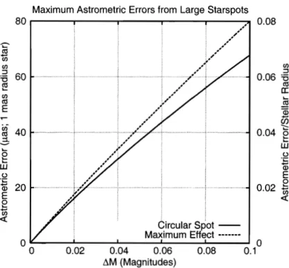
2-10 Star Spots and Astrometry . . . 46

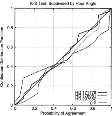
2- 11 Kolmogorov-Smirnov test: Intranight Scatter. Interwoven Data Sets . 47 2- 12 Kolmogorov-Smirnov test : Intranight Scatter. Hour- Angle Dependencies 48 2- 13 Histogram of Delay Residuals . . . 49

2-14 Allan Variances of Delay Residuals . . . 50

2- 15 Internight Repeatability Correlations . . . 54

2- 16 Internight Repeatability: 9 targets . . . 55

3-1 The Orbit of 6 Equulei . . . 63

3-2 Mass-Luminosity Isochrones for 6 Equulei . . . 66

3-3 Residuals for PHASES differential astrometry of 6 Equulei . . . 68

3-4 Residuals for previous differential astrometry of 6 Equulei . . . 69

3-5 Residuals for previous radial velocimetry of 6 Equulei . . . 70

4-1 The Orbit of K Pegasi A-B . . . 81

4-2 The Orbit of K Pegasi Ba-Bb . . . 82

4-3 Residuals for differential astrometry of K Pegasi . . . 85

4-4 Residuals for radial velocimetry of n Pegasi . . . 86

5-1 The Orbit of V819 Herculis . . . 95

5-2 PHASES measurements of V819 Herculis Ba-Bb . . . 96

5-4 Residuals for previous differential astrometry of V819 Herculis . . . . 98

5-5 Radial velocimetry residuals of V819 Herculis . . . 98

5-6 Observed Angular Momentum Orientation Distribution . . . 99

Eclipsing Binary Model Light Curve . . . 108

Eclipse Timing Sensitivity . . . 109

Radial Velocity Sensitivity . . . 113

Microlensing of MACHO-97-BLG-41 . . . 115

Geometry of Transiting Circumbinary Planets . . . 116

Tkansiting Circumbinary Planet Light Curves 1 . . . 118

Transiting Circumbinary Planet Light Curves 2 . . . 119

List of

Tables

2.1 Astrornetric Noise Sources . . . 33

2.2 Differential Dispersion . . . 38

2.3 Kol.mogorov-Smirnov Test for Intranight Repeatability . . . 48

2.4 PHASES Sources: Internight repeatability . . . 52

3.1 PHASES data for 6 Equulei . . . 60

3.2 Orbital models for 6 Equulei . . . 64

4.1 PHASES data for n Pegasi . . . 76

4.2 Keck-HIRES data for n Pegasi . . . 79

4.3 Orbital models for n Pegasi . . . 83

5.1 PHASES data for V819 Herculis . . . 91

5.2 Orbital models for V819 Herculis . . . 94

5.3 Derived physical parameters for V819 Herculis . . . 94

5.4 Known Mutual Inclinations . . . 96

Chapter

1

Background

and Motivation

Prior to the recent discoveries of the first confirmed extrasolar planetary systems, theoretical models of star and planet formation were developed that only explained systems like our own. The most accepted of these was the Safronov model [Safronov,

19721. A dense region of a molecular cloud undergoes gravitational collapse, its an- gular momel-ltum changing its shape to a disk in the process. The center of collapse becomes a protostar and dust particles combine to form planet cores in the disk. At small radii, the protostar7s heat removes gas from the disk. At large radii, enough gas remains t o form envelopes about rocky cores and create giant planets.

Surveys show that over half of star systems contain more than one stellar com- ponents. The probability of a star forming without a stellar companion and later becoming a :member of a binary via encounters with other stars is very low in most environments (except dense globular clusters). This indicates the Safronov model is an incomplete description of star formation because it predicts only one star being formed at a time. Observational studies of binaries can determine in what ways the Safronov model must be modified to include binaries, and better constrain details of the star fornxation model.

On the planet formation side, this model proved to be insufficient to explain even the first planets discovered outside our solar system. Objects with masses of terrestrial planets were detected orbiting a pulsar [Wolszczan and Frail, 19921--the Safronov model does not explain how planets can form in such an environment. The discovery of planet orbiting the main sequence star 51 Pegasi [Mayor and Queloz, 19951 was surprising because despite the planet being similar to Jupiter in mass, it was found to orbit its star very closely (with an orbital period of only four days). Searching for planets in a variety of places (even those where basic models predict they can not form) promotes the development of more detailed formation models.

For reasons of observational difficulty, narrowly separated binaries are avoided by most planet-finding methods. Searches for planets in close binary systems explore the degree to which stellar multiplicity inhibits or promotes planet formation and long term system stability. There are two generalized configurations for which planets form st able hierarchical systems in binaries. "S-type" planets orbit closely to one star of a relatively wide binary, while "P-type" or circumbinary planets have large orbits around both stars of a more compact binary. The companion star is typically

unresolved, limiting the precisions of many planet-finding techniques.

1.1

Binary Stars

It is generally accepted that the vast majority of stars that will become binaries have already established their binarity by the time that planets begin to form. Obser- vational support for this assumption comes from observations of young binary stars and protostars that have circumstellar and circumbinary disks of the type in which planets are thought to form around single stars.

The study by Duquennoy and Mayor [I9911 has demonstrated that the frequency of binaries (BF) defined as

BF = No. of MultiplesjTotal No. of Systems

among field stars older than 1 gigayear (Gyr) is 57%. The studies of multiplicity of premain-sequence stars (PMS) in the Taurus and Ophiuchus star forming regions have shown that BF for systems in the separation range 1 to 150 AU is twice as large as that of the older field stars [Simon et al., 19951. Further investigations have concluded that BF is lower for young stellar clusters (and similar to BF of the field stars) and that the binary frequency for PMS seems to be anti-correlated with stellar density [Mathieu et al., 20001. Nonetheless, BF is very high for both field and premain-sequence stars and effectively binary formation must be a major component of the star formation studies. It is perhaps because our own solar system has only one stellar component that much focus has been placed on understanding star formation as a process that causes just one star to be formed, models of which produce an unresolved mystery concerning how angular momentum is dissipated from the new star. This problem of angular momentum dissipation is easily mitigated when stars form as multiples- excess angular momentum is transferred to orbital motion. If single stars form in multiples that are later disrupted, this proposed solution to the angular moment um transport problem can be applied generally.

Similarly, one may conclude that the typical setting for the planet formation is probably that of a binary system and it may not be possible to assess the overall frequency of extrasolar planets without addressing the binary systems. Yet, current radial velocity (RV) surveys for extrasolar planets favor single stars. This bias is driven by the observing technique and since there is a growing evidence of the occur- rence of planets in binary and multiple stellar systems, one can no longer ignore the subject of their formation and properties.

1.2

Extrasolar Planets

Starting in the early nineties there have been three major developments in the field of sub-stellar objects: (1) the discovery of the first planetary system around another star, namely PSR 1257+12 [Wolszczan and Frail, 19921 (2) the discovery of the first confirmed brown dwarf, the companion to Gliese 229B [Nakajima et al., 19951, and

(3) the disct:)very of a planet around a normal star [Mayor and Queloz, 19951. These

discoveries have propelled major observational programs and the field of brown dwarfs and extra-solar planets has exploded [see summaries Basri, 2000, Perryman, 2000, hlarcy and Butler, 19981. Thus far, over a hundred extrasolar planets have been found by different groups using precise radial velocities

[http: //vo.obspm. fr/exoplanetes/encyclo/encycl. 1 Schneider, 20031.

The study of extrasolar planets has matured beyond the point of simply identi- fying planetary systems and now can explore deeper questions about the frequency of planetary systems, how planets form, and how far the range of planetary diversity extends. To start with, there are two extreme possibilities: planetary systems are rare (and essentially accounted for by the known systems) or planet formation is rich and diverse and the current sample is limited by observing techniques. The existence of an entire planetary system around a millisecond pulsar-PSR 1257+12-favors the second hypothesis. If so, the current sample selects those planets best identified by RV technique, namely planets with short orbital periods. Additional discoveries that support the hypothesis that planetary systems occur in a broad range of environments include giant; planets in orbits as short as one day [Torres et al., 2003], planets with large orbital eccentricities, the possible imaging of a planet orbiting a brown dwarf [Chauvin et al., 20041, and a planet system in a globular cluster [Sigurdsson et al., 20031.

1.3

Planets in Binaries

Current theory is that planets form in and from material of dusty disks observed around young stars. Popular (professional) prejudice has it that planet formation is difficult or inhibited in binary or multiple stars because these disks might be more short-lived. However, ezghteen of the current sample of over a hundred extrasolar

planets are in binary or multiple systems (see Figure 1-3). Given that multiplicity is the norm in the solar neighborhood [57%, Duquennoy and Mayor, 19911 and star- forming regions [Simon et al., 19951, the entire issue of planets in binary and multiple stars cannot be ignored.

The radial velocity detections of planets in binary systems are quite surprising re- sults given that binary stars are often avoided by these surveys (because the secondary will contaminate the spectrum of the primary and thereby limit the measurement pre- cision). Since despite this bias planets are detected in stellar binaries, there is a well justified and important question of the occurrence and properties of planets in such systems. It has been recognized by Zucker and Mazeh [2002] who has noted that there may be a deficiency of "high" mass planetary companions with short period orbits around single stars whereas the opposite may be true for planets in binary sys- tems. Indeed, recent discoveries - a brown dwarf companion with an orbital period of

1.3-day around the star HD 41004B (AB separation 21 AU) and the planet of G186A with mass (n-L sin i) of 4 M j , (binary orbital separation of 20 AU) - lend credence to

1.3.1

Circumstellar and circumbinary disks

One of the prime examples of the circumstellar disks in a binary system is the case of L1551 IRS 5. Rodriguez et al. [I9981 show that L1551 IRS 5 is a binary PMS with separation of 45 AU in which each component is surrounded by a disk (see Figure

1-1). The radii of the disks are 10 AU and the estimated masses are 0.06 and 0.03

Ma,

enough t o produce planets. Recently, McCabe et al. I20031 have spatially resolved mid-infrared scattered light from the prot oplanet ary disk around the secondary of the PMS binary HK Tau AB . The inferred sizes of the dust grains are in the range 1.5-3 pm which suggests that the first step in the planet formation, the dust grain growth, has occurred in this disk. Altogether, there is ample evidence for the presence of disks in binary systems. Observational indicators such as excess emission at near-infrared to millimeter wavelengths but also spectral veiling, Balmer and forbidden emission lines and polarization suggest that disks can be found around each of the components (circumprimary and circunisecondary disks) as well as around the entire systems [cir- cumbinary disks, for a review see Mathieu et al., 20001. Specifically, millimeter and submillimeter measurements of dust continuum emission enable measurement of the total disk mass. These observations show that circumbinary disks may be reduced in size and mass but still are present even in close systems. The presence of circumbi- nary disks is observed at millimeter wavelengths around many PMS spectroscopic binaries. Such massive disks are however rare around wide binaries with separations 1- 100 AU. This is reflected in theoretical calculations that predict circumstellar and circumbinary disks trunca'ted by the companions [Lubow and Artymowicz, 20001. The circumstellar disks have outer radii 0.2-0.5 times the binary separation while the circumbinary disks have the inner radii 2-3 times the semi-major axis of the bi- nary. Finally, the measurements of the infrared excess emission show no difference in frequency of the excess among binaries and single stars. It indicates that the circum- stellar material in binary systems may be similar in temperature and surface density t o that in disks surrounding single stars [Mathieu et al., 20001. Hence it seems that with the current data at hand, planet formation in close binary systems is possible.

1.3.2 Planet Format ion in Binaries

The theories of planet formation in binary stellar systems are still at early stages. Two mechanisms proposed for giant planet formation in circumstellar disks-core ac- cretion and fragmentation via gravitational instabilities-make conflicting predictions about the formation rate of planets in binaries. This is primarily due to the differ- ences in formation timescales; core-accretion requires 1-10 million years as compared to thousand year timescales for gravitational collapse. Mayer et al. [2004] indicate that gravitational fragmentation models of planet formation predict different efficien- cies for giant planet formation in binaries than in single stars, whereas core-accretion models do not. It is argued that a stellar companion will disrupt protoplanetary disks on timescales shorter than required for core-accretion. Whitmire et al. (19981 studied terrestrial planet growth in the circumprimary habitable zones in binary sys- tems. They considered a 4-body system of 2 stars and 2 planetesimals for which by

04 28 40.26

40.25

40.24

40.23

_40.22

Right ascension

(81950)

Figure 1-1: Very Large Array (VLA) map of the L1551 IRS 5 region a t 7 mm [figure is from Rodriguez et al., 19981.

varying binary parameters (semi-major axis, eccentricity, mass ratio) they were able t o determine a critical semi-major axis of the binary below which the secondary does not allow a growth of planetesimals (planetesimals are accelerated by the secondary, the relative velocity of planetesimals is larger than critical and their collisions become destructive). Based on this criterion, they concluded that about 60% of nearby solar- type binaries cannot be excluded from having a habitable planet. Marzari and Scholl [2000] analyzed a Cen AB (semi-major axis of 23 AU, eccentricity of 0.52, mass ratio

1.1/0.92), a prototype close binary system, and demonstrated that planetesimals can accrete into planetary embryos. Barbieri et al. [2002] continued the study and showed that planetary embryos can grow into terrestrial planets in about 50 Myr. Fragmen- tation models by Boss [I9981 claim that giant planet formation is enhanced by the presence of stellar companions-when no binary is present, the disk is more stable and less likely t o fragment into planets. However, Nelson [2000] argues that gas heating causes both mechanisms t o fail t o produce planets in binaries of moderate separation (50 A.U.). Clearly, there is a lack of consensus and the planet formation theories would certainly benefit from observational constraints.

1.3.3

Binary Planet Stability

Theoretical work of planet formation in close binary systems is a t a rudimentary stage. Yet, as demonstrated by numerical studies [Holman and Wiegert, 19991, plan- ets (if formed) in binary systems can enjoy a wide range of stable orbits. There is a clear need t o supply observational constraints on the occurrence and orbital prop- erties of extrasolar planets in binary systems t o provide the key information for the theories of their formation. Unfortunately, it is well known that current RV surveys are biased against binary stars [e.g. see Patience et al., 20021. The radial velocity sur- veys exclude binaries with separations of less than 2 arcsecond t o avoid the problem posed by the "contamination" caused by the second star [Vogt et al., 20001. Imaging and particularly coronographic surveys are similarly biased (mainly because current coronographs can suppress light from only one object in the field).

The problem of stability of the planetary orbits in binaries has been recognized for a long time. Most often, it was approached with the aid of numerical studies of the elliptic restricted three-body problem. The orbital configurations considered include the so-called P-type (Planet-type, circumbinary orbits)

,

S-type (Sat ellit e- type, circumprimary or circumsecondary orbits) and L-type orbits (Librator-type, orbits around stable Lagrangian points L4 or L5 for the mass ratio p

<

0.04). There are many papers concerning the stability of S-type motions [e.g. Benest, 2003, Pilat- Lohinger and Dvorak, 2002, Benest, 1996, 1993, 1989, 1988, Rabl and Dvorak, 19881. These studies concentrated on developing empirical stability criteria in the framework of the circular three-body problem [see e.g. Graziani and Black, 1981, Black, 1982, Pendleton and Black, 19831. The P-type motions have also been investigated [Pilat- Lohinger et al., 2003, Broucke, 2001, Holman and Wiegert, 1999]. Until now however, there is no observational evidence that they exist. The curious L-type orbits have also attracted the interest of researchers [see e.g. Laughlin and Chambers, 20021.

Figure 1-2: The relative population frequency of observed binary stars. Planets are most easily detected in nearby systems (within

=

100 parsecs), for which the binary distribution peaks at separations on order of tenths of arcseconds. [Figure is from Duquennoy and Mayor, 19911.

tions, excluding works by some authors, e.g., Pilat-Lohinger et al. [2003], who applied the FLI indicator (FLI, Fast Lyapunov Indicator). They have many limitations: most of the analytical works are done for circular binaries, numerical studies have been re- stricted to special mass ratios and the integration have been limited to fairly short times. Also, they are almost exclusively restricted to the framework of the three body problem. These drawbacks have been addressed in the recent, remarkable work by Holman and Wiegert [I9991 who studied a full range of mass ratios, eccentricities and long integration times (at least lo4 periods of the binary). They demonstrated that planets in binaries can enjoy a wide range of stable orbits. The stability criteria are most sensitive to the ratio of planet-binary semimajor axis; one can derive "observers' rules of thun:1bn from the collected theoretical work that P-type planets are stable if they have semimajor axis 3 times larger than that of the binary, and S-types are

stable if they are in orbits closer than 117 the binary separation.

1.3.4 Planet Frequency versus Binary Separation

The lifetimes of circumstellar disks in binary systems are expected to decrease as the binary separation shrinks. Thus, one may set limits on the timescales over which gi- ant planet formation occurs by decreasing the separations of binaries in which planets are sought. This also allows one to search for any enhancements in formation rates

due to increased disk turbulence that are predicted in some planet formation theo- ries. Finally, the distribution of separations of nearby binaries peaks at less than an arcsecond, a separation smaller than that easily probed by traditional high precision radial velocity techniques.

There are also observational reasons for searching for planets in binaries. In particular, the binary companion makes a convenient nearby reference for astrometric observations. The chance of finding an unrelated but still bright reference star close on the sky to a target is small, which limits the number of targets available to astrometric study. Astrometry has several advantages over other techniques. While radial velocity observations can only set a lower limit on a companion mass, which is degenerate with orbital inclination, astrometry measures companion mass directly. Astrometry is also more sensitive to long period companions. The anticipated diversity in extra- solar system planets has driven astronomers and agencies to consider a multitude of discovery techniques. Each technique has its strengths. This complementarity of sensitivity is one of the principal motivations for the Keck Interferometer and the Space Interferometer Mission (SIM).

1.4

PHASES: The Palomar High-precision Astro-

metric Search

for

Exoplanet Systems

The Palomar High-precision Astrometric Search for Exoplanet Systems (PHASES) is a search for S-type giant planets orbiting either star in 50 binary systems. The goal of this search is to detect or rule out planets in the systems observed and thus place limits on any enhancements of planet formation in binaries. This sensitivity- limited search may be extended to a more complete survey of up to 500 stars with an upgraded observational system. The method used to conduct this survey is described in chapter 2 of this thesis. Though the time span of the search does not yet allow us t o detect planets, three years of future operation in this mode are anticipated. chapters 3, 4, and 5 each discuss a binary of interest studied with this method, The final chapter discusses techniques for detecting P-type planets; such a search would be complementary to PHASES.

Distance to Binary [pc]

Figure 1-3: The distribution of binaries from the PHASES sample compared to the three binaries with planets which have the smallest binary separation. The 2- arcsecond selection effect is visible.

0.1 p

10

Solar Planets

Planets in Wide Binary System7

8

3- r RV 20 m s- - m - - - . - s

3-yr PHASES, 10 pc, ~oyar Mass Stars

-

'

PHASES sensitivity ----t

0.01 " " I I 1

0.1 1 10 1

Semi-Major Axis (AU)

10 100 1000

Binary Semi-Major Axis (AU)

I - . . - - - . - I - --...-- I - - . - . - - r

Target systems in PHASES primary sample

-

Known planets in binaries

.

I . . . ... I . . . ... I - . - .-

Figure 1-4: A comparison of the performance of PHASES astrometric performance for detecting planets in sub-arcsecond binaries and radial velocity observations of wider systems. In the left graph, radial velocity and astrometry measurements can detect planetary companions in the phase spaces above the plotted curves. Astrometry is sensitive t o much lower mass planets near the habitable zone, and can be used t o search for planets in binaries with much smaller physical separations. Note in the right graph that for several PHASES targets, the maximum stable planet period is less than three years; orbital stability plays a bigger role in these closely bound systems.

Chapter

2

Narrow Angle Astrometry

A new observing method was developed to perform very high precision differential astrometry on bright binary stars with separations in the range of

-

0.1 - 1.0 arcsec-

onds. Typical measurement precisions over an hour of integration are on the order of 10 micro-srcseconds (pas), enabling one to look for perturbations to the Keplerian orbit that would indicate the presence of additional components to the system. This method of very-narrow-angle astrometry forms the basis of a search for extrasolar planets orbit,ing either stellar component of the binary. It is also used to measure fundamental properties of the stars comprising the binary, such as masses and dis- tances, useful for constraining stellar models at the level. This method forms the basis for the Palomar High-precision Astrometric Search for Exoplanet Systems

(PHASES).

2.1

Introduction

Long-baseline optical interferometry promises high precision astrometry using mod- est ground-based instruments. In particular the Mark I11 Stellar Interferometer [Shao et al., 19881 and Navy Prototype Optical Interferometer [Armstrong et al., 19981 have achieved global astrometric precision at the 10 mas (1 mas = arcseconds) level [Hummell et al., 19941, while the Palomar Test bed Interferometer (PTI) [Colavit a et al., 19991 has demonstrated an astrometric precision of 100 pas ( l p a s = arc- seconds) between moderately close (30 arcsecond) pairs of bright stars [Shao and Colavit a, 1992, Colavita, 1994, Lane et al., 20001. While interferometric and astro- metric methods have proven very useful in studying binary stars, and have long been argued to be well-suited to studying extra-solar planets [Colavita and Shao, 1994, Eisner and Kulkarni, 2001], to date results using these techniques have been limited [Benedict et al., 20021.

There are several reasons why it is desirable to develop viable astrometric planet- detection methods. Most importantly, the parameter space explored by astrometry is complementary to that of radial velocity (astrometry is more sensitive to larger sepa- rations). Second, unlike current radial velocity detections, astrometric techniques can

Figure 2-1: 'The Palomar Testbed Interferometer as seen from the catwalk of the Palomar Hale 200" telescope.

t icularly well -suited for studying binary stellar systems; such systems challenge other planet-finding techniques. For example, radial velocimetry can suffer from system- atic velocity errors caused by spectral contamination from the light of the second star [Vogt et al., 20001. Similar problems are faced by coronographic techniques, where the light frorn the second star is not usually blocked by the occulting mask.

This chapter describes recent efforts to obtain very high precision narrow-angle astrometry using PTI t o observe binary stars with separations less than one arcsecond, i.e. systems that are typically observed using speckle interferometry [Saha, 20021 or adaptive opt,ics. Such small separations enable astrometric precision on the order of 10 pas which, for a typical binary system in the PHASES target sample (binary separation of 20 AU), should allow detection of planets with masses down t o 0.5 Jupiter masses in orbits in the 2 AU range. This approach has been suggested [Traub et al.. 19961 and tried [Dyck et al., 1995, Bagnuolo et al.. 20031 before, though with limited precision. However, this work is unique in that it makes use of a phase-tracking interferometer; the use of phase-referencing [Lane and Colavita, 20031 removes much of the effect of atmospheric turbulence, improving the astrometric precision by a factor. of order 100.

PTI is located on Palomar Mountain near San Diego, CA [Colavita et al., 19991.

It was developed by the Jet Propulsion Laboratory. California Institute of Technology for NASA, as a testbed for interferometric techniques applicable to the Keck Interfer- ometer and other missions such as the Space Interferometry Mission, SIM. It operates in the J (1.2pm),H (1.Gpm) and K (2.2pm) bands, and conibines starlight from two out of three available 40-crn apertures. The apertures form a triangle with two 87 and one 110 meter baselines.

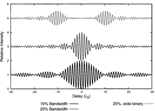
10% Bandwidth

-

20% Bandwidth

---

20%, wide binary --....--

Figure 2-2: The response of an interferometer. The top two curves have been offset by 2 and 4 for clarity. The widths of the fringe packets are determined by the bandpass of the instrument, and the wavelength of fringes by an averaged wavelength of starlight. The top curve shows the intensity pattern obtained by observing two stars separated by a small angle on the sky-the observable is the distance between the fringe packets.

2.2

Optical

Interferometers

In an optical interferometer light is collected at two or more apertures and brought to a central location where the beams are combined and a fringe pattern produced on a detector (at PTI, the detectors are NICMOS and HAWAII infrared arrays, of which only a few pixels are used). For a broadband source of central wavelength X

arid optical bandwidth AX (for PTI AX = 0.4pm), the fringe pattern is limited in extent and appears only when the optical paths through the arms of the interferom- eter are equalized to within a coherence length (A = X2/AX). For a two-aperture interferometer, neglecting dispersion, the intensity measured at one of the combined beams is given by

sin (ax/A)

sin (2ax/X)

where V is the fringe contrast or "visibility", which can be related to the morphology

of the source, and x is the optical path difference between arms of the interferometer. More detailed analysis of the operation of optical interferometers can be found in

% C, .- (I) c a, 0 Frequency (Hz)

Figure 2-3: Power spectral density of the fringe phase as measured by P T I [Lane and Colavita, 20031. The phase PSD is best fit by a power law A ( f ) K f-2.5, close t o the

the nominal -813 slope of Kolmogorov theory. Also shown is the effective PSD of the phase noise after phase referencing has stabilized the fringe.

2.2.1

Interferometric Astrometry

The location of the resulting interference fringes are related t o the position of the target star and the observing geometry via

where d is the optical path-length one must introduce between the two arms of the interferometer t o find fringes. This quantity is often called the "delay."

3

is the baseline--the vector connecting the two apertures.

9

is the unit vector in the source direction, and c is a constant additional scalar delay introduced by the instrument. The term

6,

(3,

t )

is related t o the differential amount of path introduced by the atmosphere over each telescope due t o variations in refractive index. For a 100-m baseline interferometer an astrometric precision of 10 pas corresponds t o knowing d

t o 5 nm, a difficult but not impossible proposition for all terms except that related t o the atmospheric delay. Atmospheric turbulence, which changes over distances of tens of centimeters and on millisecond timescales, forces one t o use very short exposures (to maintain fringe contrast) and hence limits the sensitivity of the instrument. It also severely limits the astrometric accuracy of a simple interferometer, at least over large sky-angles.

and the observable is a differential astrometric measurement, i.e. one is interested in

+

knowing the angle between the two stars

(A,

=

3

-

3).

The atmospheric turbulence

is correlated over small angles. If the measurements of the two stars are simultaneous, or nearly so, the atmospheric term subtracts out. Hence it is still possible t o obtain high precision "narrow-angle" astrometry.

2.2.2 Narrow-Angle Astrometry

'Il-aditional interferometric narrow-angle astrometry [Shao and Colavita, 1992, Colavita, 19941 promises astrometric performance at the 10- 100 micro-arcsecond level for pairs of stars sepa,rated by 10-60 arcseconds; it was first demonstrated with the Mark I11 interferometer for short integrations [Colavita, 19941, was extended to longer integra- tions and shown t o work a t the 100 micro-arcsecond level at P T I [Shao et al., 19991, and is expected to become operational a t the Keck Interferometer in 2010. However, achieving such performance requires simultaneous measurement of the fringe posi- tions of both stars, greatly complicating the instrument (two beam combiners and metrology tllroughout the entire array are required). In addition, the instrumental baseline

3

must be known t o high precision (= 100 microns). While this mode has been demonstrated on a limited basis at PTI, the addition of the metrology system severely limits the throughput of the instrument and hence the number of observable targets.

For more closely spaced stars, it is possible to operate in a simpler mode. PTI has been used t o observe pairs of stars separated by no more than one arcsecond. In this mode, the small separation of the binary results in both binary components being in the field of view of a single interferometric beam combiner. The fringe posit ions are measured by modulating the instrument a1 delay with an amplitude large enough t o record both fringe packets. This eliminates the need for a complex internal metrology system t o measure the entire optical path of the interferometer, and dramatically reduces the effect of systematic error sources such as uncertainty in the baseline vector (error sources which scale with the binary separation).

However, since the fringe position measurement of the two stars is no longer truly simultaneous it is possible for the atmosphere t o introduce path-length changes (and hence positional error) in the time between measurements of the separate fringes. To reduce this effect a fraction of the incoming starlight is redirected to a separate beam-combiner. This beam-combiner is used in a "fringe-tracking" mode [Shao and Stiaelin, 1980, Colavita et al., 19991 where it rapidly (10 ms) rneasures the phase of one of the starlight fringes, and adjusts the internal delay t o keep that phase constant. The fringe tracking data is used both in real-time (operating in a feed-back servo, after which a small-but measurable--residual phase error remains) and in post-processing (the measured residual error is applied t o the data as a feed-forward servo). This technique-known as phase referencing--has the effect of stabilizing the fringe measured by the astrometric beam-combiner. For this observing mode, laser metrology is only required between the two beam combiners through the location of the light split; (which occurs after the optical delay has been introduced), rather than throughout the entire array.

-1 5

0 10 20 30 40 50 60

Seconds

Figure 2-4: An example of how phase referencing stabilizes the fringe. Shown are plots of the fringe position seen by the a P T I fringe tracker with and without phase referencing. The two data sections were taken within 200 seconds of each other. The target star was HD 177724 (mK = 2.99, AOV). One detector was operated with 20 ms sample times and open loop, i.e., measuring but not correcting the phase. In the first experiment, without phase referencing, the raw atmospheric phase fluctuations are observed. For the second data set plotted, a second beam combiner was operated in closed loop, with its phase information being applied t o the open loop beam com- biner, reducing the phase fluctuations it observed. Note the jump near 20 seconds in the phase-referenced data; this is caused by mis-identification of the central fringe. This is easily detected and corrected during post-processing by measurements of the interferometer's group delay, or fringe phase versus wavelength.

100 -50 0 50 100

Optical Delay (microns)

Figure 2-5: Measured intensity in the detector as a function of differential optical path, for successive scans of the speckle binary system HD 44926. Each scan takes 1.5 seconds to acquire. The fringe tracker was locked on to the bright star (around 0), while the second star produces a fringe pattern which starts at -40 pm and moves due to Earth rotation. Although the second fringe pattern is relatively faint, the effect of coherently co-adding 500-2000 scans produces a high signal-to-noise ratio in the final astrometric measurement.

In making an astrometric measurement the optical delay is modulated in a triangle- wave pattern around the stabilized fringe position, while measuring the intensity of the combined starlight beams. The range of the delay sweep is set to include both fringe packets; typically this requires a scan amplitude on the order of 150 pm. Typ- ically one such "scan" is obtained every second, consisting of up to 1000 intensity sa,mples (the scan rate is limited by the source brightness and the requirement that

>

2 samples are made per wavelength of scan amplitude). A double fringe packet based on eq. 2.1 is then fit to the data, and the differential optical path between fringe packets is measured.

2.3

Data Reduction Algorithm

The relative astrometric position is extracted from data such as that shown in Figure 2-5 as follows. Observing a binary when its baseline projected separation

(3

a)

is of order the interferometric coherence length ( z 20pm) or less is avoided due to potential biases associated with an imperfect template fringe packet. First, detector calibrations (gain, bias, and background) are applied to the intensity measurements.

Next, a grid in differential right ascension and declination over which to search is constructed (in ICRS 2000.0 coordinates). For each point in the search grid the expected differential delay is calculated based on the interferometer location, baseline geometry, and time of observation for each scan. These conversions were simplified using the routines from the Naval Observatory Vector Astrometry Subroutines C

Language Version 2.0 (NOVAS-C; see Kaplan et al. [1989]). A model of a double- fringe packet is then calculated and compared to the observed scan to derive a X2

value; this is repeated for each scan, co-adding all of the X2 values associated with

that point in the search grid. The final

x2

surface as a function of differential R.A. and declination is thus derived. The best-fit astrometric position is found at the r n i n i r n ~ m - ~ ~ position, with uncertainties defined by the appropriate

x2

contour- which depends on the number of degrees of freedom in the problem and the value of the x2-minimum. The final product is a measurement of the apparent vector between the stars and associated uncertainty ellipse. Because the data were obtained with a single-baseline instrument, the resulting error contours are very elliptical, with aspect ratios at times

2

10.

2.3.1

Probability Distribution Function Sidelobes

One potential complication with fitting a fringe to the data is that there are many local minima spaced at multiples of the operating wavelength. If one were to fit a fringe model to each scan separately and average (or fit an astrometric model to) the resulting delays, one would be severely limited by this fringe ambiguity (for a 110-m baseline interferometer operating at 2.2pm, the resulting positional ambiguity is -- 4.1 milli-arcseconds). However, by using the x2-surface approach, and co-adding the probabilities associated with all possible delays for each scan, the ambiguity dis- appears. This is due to two things, the first being that co-adding simply improves the signal-to-noise ratio. Second, since the observations usually last for an hour or even longer, the associated baseline change due to Earth rotation also has the effect of "smearing" out all but the true global minimum. The final X2-surface does have dips separated by 4.1 milli-arcseconds from the true location, but any data sets for which these show up at the 4 0 level are rejected. The final astrometry measurement and related uncertainties are derived by fitting only the 40 region of the surface.

2.3.2

Residual Unmonitored Phase Noise

Unmonitored system phase noise affects the X2 surface in two ways. First, components

of the phase noise that operate at frequencies faster than the scan rate cause the two fringe packets to be smeared an extra amount, and to first order this appears as extra noise in the intensity measurements. This affects the width of the X2 fit for each

individual scan (which is designated om, the "measurement" noise), and thus appears directly in the co-added X2 contour.

If instead the instrumental noise is much slower than an individual scan, it is essential "frozen into" the scan--for the duration of that scan, the stars really do appear to have a different separation than their true separation. The X2 surface for

the fit t o an individual scan takes the form

where dj is the value of the star separation that minimizes f = X2, and n is the

number of degrees of freedom of the fit (typical values for n are 400-1000; for this derivation, it suffices t o assume a one-dimensional

x2

surface as it has no curvature in the direction perpendicular t o the sky-pro j ected baseline-only Eart h-rotation syn- thesis lifts this degeneracy). The low-frequency components of the phase noise cause daj to vary from do, the true star separation, by more than one expects from measure- ment noise alone. By taking many such scans, one can determine this instrumental scatter (which is designated as a,, the "instrument" noise for an individual scan) and add (in quadrature) the instrumental noise t o the measurement noise, as

where N is the number of scans ( N is typically hundreds to thousands).

Consider a function f (d - doj ) with centroid position doj ; this centroid position is

distributed with probability

One may naively hope that summing several instances of this function with vari- able do] together would properly add the instrumental and measurement noises in quadrature. However, the summation results in

Even if one renormalizes so that the additive term equals n N (i.e. multiply by n / ( n

+

0:/0k)),

this is still:

Note the extra factor of n dividing 0:; this effectively underestimates the scan-to-scan

instrumental noise by a very large amount-roughly 20x for typical PHASES data. Instead, the appropriate way to determine the scan-to-scan fit is by noticing that

the minimum value of the co-added X 2 surface is greater than the total number of

degrees of freedom n N by the amount:

The quantity om is measured directly from the shape of the surface, which is un-

changed, and the number of scans N is known. Thus, one can derive oi and apply it t o the formal uncertainties. For 430 observations made from 2003-2005, the average value of a:/& was 1.43; values ranged from 0.0084 (for bright sources and good

weat her conditions) to 7.2.

Phase-referencing is used to decrease the amount of unmonitored phase noise dur- ing narrow-angle astrometry observations (see section 2.4.1)

,

but some residual phase noise remains (see Figure 2-3), so the correction outlined here must be applied to the astrometric data. Synthetic data have been constructed both with and without unmonitored phase noise of the actual spectrum observed, and the data reduction algorithm determines measurement uncertainties consistent with the actual scatters in the measurements between multiple synthetic data sets. Without the additional phase-noise correction outlined here, the formal uncertainties significantly underesti- mate the scatter in the results.

2.4 Expected Performance

The expected astrometric performance of the new observing mode is determined by several factors contributing measurement uncertainties and biases. These are sub- divided into three broad categories: (1) observations noise terms, which are funda- mental t o atmospheric turbulence and finite source brightness, (2) instrument a1 noise terms, which result from the design of the interferometer and the method in which the measurement is obtained, and (3) astrophysical noise terms, which result from the astrometric stability of the stars themselves. The size of each noise source is summarized in Table 2.1.

2.4.1

Observational Noise

In calculating the expected astrometric performance three major sources of error are taken into account: errors caused by fringe motion during the sweep between fringes (loss of coherence with time), errors caused by differential atmospheric turbulence (loss of coherence with sky angle, i.e. anisoplanatism), and measurement noise in the fringe position. Each is quantified in turn below, and the expected measurement precision is the root-sum-squared of the terms (Figure 2-6).

2.4.1.1 Loss of Temporal Coherence

The power spectral density of the fringe phase of a source observed through the atmosphere has a power-law dependence on frequency (Figure 2-3); at high frequencies

Table 2.1

Astrometric Noise Sources

Source Section Typical Magnitude (pas) Temporal Decoherence 2.4.1.1 - 5 .4nisoplanatism 2.4.1.2 0.2 Photon Noise 2.4.1.3 3 Differential Dispersion* 2.4.2.1 30 Baseline Errors 2.4.2.2

<

10 Fringe Template 2.4.2.3 1 Scan Rate 2.4.2.4 1 Beam Walk 2.4.2.5 0.5 Global Astrometry 2.4.2.6 < < I Star spots 2.4.3.1

<

8t Stellar Granulation 2.4.3.2

<

3

Table 2.1: Sources of astrometric noise.

* Depends on color difference between binary components; for many targets, this is nearly zero, but for extreme color differences, this can be hundreds of pas.

Photometric variability accompanies star spots, of a magnitude that is easily de- tected for astrometric signatures of 8 pas or larger.

typically

A(f )

f

-a

where cu is usually in the range 2.5-2.7. The effect of phase-referencing is t o high- pass filter this atmospheric phase noise. In this case, the servo is an integrating servo with finite processing delays and integration times, with the residual phase error "fed forward" t o the second beam combiner [Lane and Colavita, 20031. The response of this system t o an input atmospheric noise can be written in terms of frequency (see Appendix A in Lane 2003) as

where sinc(x) = sin(x)/x, f c is the closed-loop bandwidth of the fringe-tracker servo

(for this experiment f c = 10 Hz), Ts is the integration time of the phase sample

(6.75 ms), and Td is the delay between measurement and correction (done in post- processing, effectively 5 ms). The phase noise superimposed on the double fringe measured by the astrometric beam combiner has a spectrum given by A( f ) H ( f ) .

The sampling of the double fringe packet takes a finite amount of time, first sampling one fringe, then the other. In the time domain the sampling function can be represented as a "top-hat" function convolved with a pair of delta functions (one positive, one negative). The width of the top-hat is equal to the time taken t o sweep through a single fringe, while the separation between the delta functions is equal to

the time t o sweep between fringes. In the frequency domain this sampling function becomes

S(f) = sin2(2.rr f ~ , ) s i n c ~ ( n f ~ , ) (2.10)

where rP is the time taken to move the delay between stars ,Ad/vs, and T, is the time

to sweep through a single stellar fringe, A/vs. us is the delay sweep rate.

The resulting error in the astrometric measurement, given in radians by otc, can be found from

where N is the number of measurements. It is worth noting that if phase-referencing is not used t o stabilize the fringe, i.e.

H(

f ) = 1, the atmospheric noise contribution increases by a factor of x lo2-lo3.

2.4.1.2 Anisoplanatism

The performance of a simultaneous narrow-angle astrometric measurement has been thoroughly analyzed in [Shao and Colavita, 19921. Here the primary result for the case of typical seeing at a site such as Palomar Mountain is restated, where the astrometric error in arcseconds due to anisoplanatism (0,) is given by

where B is the baseline (in meters), 6 is the angular separation of the stars (in radians), and t the integration time in seconds. This assumes a standard [Lindegren, 1980] atmospheric turbulence profile; it is likely that particularly good sites will have somewhat (factor of two) better performance.

2.4.1.3 Photon Noise

The astrornetric error due to photon-noise (0,) is given in radians as

where N is the number of fringe scans, and SNR is the signal-to-noise ratio of an individual fringe.

2.4.2

Instrumental Noise

There are several effects internal to the instrument that can contribute noise terms or biases to the astrometric measurements. Some could potentially vary on night-to- night timescales as the optical alignments vary on roughly these timescales. Others result from properties of the measurement design.

Separation (mas)

Figure 2-6: The expected narrow-angle astrometric performance in milli-arcseconds for the phasoreferenced fringe-scanning approach, for a fixed delay sweep rate, and an interferometric baseline of 110 m. There are three primary sources of astrometric error in this method: angular anisoplanatism [Shao and Colavita, 19921, temporal de- coherence [Lane and Colavita, 20031, and photon noise. Also shown is the magnitude of the temporal decoherence effect in the absence of phase referencing, illustrating why stabilizing the fringe via phase referencing is necessary.