Automated perfusion-weighted MRI metrics via localized arterial input functions

(1)

Automated Perfusion-Weighted MRI Metrics via

Localized Arterial Input Functions

by

Cory Lorenz

B.S. Electrical Science & Engineering, MIT (2003)

Submitted to the department of Electrical Engineering and Computer Science in Partial Fulfillment of the Requirements for the Degree of

Masters of Engineering in Electrical Engineering and Computer Science at the

Massachusetts Institute of Technology June 2004

The author hereby grants to MIT permission to reproduce and distribute publicly paper and electronic copies of this thesis document in whole or in part.

/I I

A uthor ... I ... l...

Department of Electrical Engineering and Computer Science May 12, 2004

Certified by ...

A. Gregory Sorensen

Associate Professor of Radiology, Harvard Medical School

HST Affiliated Faculty, Thesis Supervisor

Accepted by ...

Arthur C. Smith Chairman, Departmental Committee on Graduate Students

MASSACHUSETS INS E

OF TECHNOLOGY

JUL 2

2004

(2)

(3)

Automated Perfusion-Weighted MRI Metrics via Localized Arterial Input Functions

by Cory Lorenz

Submitted to the Department of Electrical Engineering and Computer Science on May 12, 2004, in Partial Fulfillment of the Requirements for the Degree of Masters of

Engineering in Electrical Engineering and Computer Science ABSTRACT

This thesis describes and validates a new method for calculating perfusion-weighted MRI (PWI) metrics, a non-invasive technique for calculating cerebral blood flow by tracking a bolus of contrast agent. Past methods to do this calculation require human intermediaries and can lead to errors in the presence of delay and dispersion of the contrast bolus, situations which occur commonly in the pathological conditions which require PWI. The new method described calculates perfusion metrics by defining an arterial input function (AIF) for every voxel in the brain based upon the voxels in close proximity to it. This allows for automated calculation of perfusion metrics, and the localized nature of the ALFs creates an implicit regard for delay and dispersion. This thesis demonstrates that this local AIF method is indeed able to correct flow misestimations due to delay and dispersion, and that it is also more useful for predicting tissue outcome post-stroke.

Thesis Supervisor: A. Gregory Sorensen, M.D., Ph.D.

(4)

(5)

Acknowledgements

First and foremost, I'd like to thank my thesis advisor, Greg Sorensen, for giving me this opportunity and for all his support. His good advice and positive outlook were always helpful and appreciated.

Secondly, I'd like to thank Thomas Benner (a man who needs no acronym) for all of his advice, coding help, proofreading, brainstorming sessions, and for his good sense of humor about things.

At the MGH-NMR center I'd like to thank Chloe Lopez for all of her help with the GLM, showing me how to use various programs, as well as making and linking lots of perfusion maps for me. I'd also like to thank Nina Menezes and Hakan Ay for their proofreading and suggestions on manuscripts, as well as answering my questions about submitting abstracts, attending conferences and many of the other things that I had to do for the first time this year. Mark Vangel also has my gratitude for his statistical consultations. In addition, I'd like to thank Tara Ullrich for helping me out with all of my paperwork and getting me setup at the lab.

Of course, I have to thank the many friends that I have made at MIT, who have made my

life here so much better. First, I'd like to thank Kevin Pipe, for being a role-model of sorts to me. His wisdom, good advice and jump shot (as long as I didn't have to defend it) were always valuable. I also extend my gratitude to my roommates Nathan Mahn and Louis Lopez, for being not only great roommates, but also great friends. Thanks for putting up with my ranting and complaining, as well as my mess, (even though I didn't

always make it) but also for all of the food and good times. In addition, I'd like to thank my many other close friends: Aditi Garg for her advice and great friendship; Rob Kyker,

for his encouragement and idealism; Andrew Brooks, for always having his door open when I needed advice; Alex Firshein and Tanya Burka for being loyal and helpful

friends; Matt Brooks and Tristan Hayeck for being there when I needed them. I will (or already do) miss all of you.

Last, and certainly not least, I'd like to thank my parents. For supporting me all these years, for always believing in me, and for putting up with me when things were most

(8)

(9)

Chapter 1: Introduction

1.1 Motivation

Perfusion-weighted magnetic resonance imaging (PWI) is a common imaging technique used in the clinical treatment of patients with brain pathologies such as stroke or cancer (1,2). PWI allows physicians to characterize blood perfusion in the brain non-invasively as part of a patient's standard MR protocol. Perfusion weighted images are obtained by injecting a bolus of gadolinium chelate into a patient's bloodstream and imaging as it passes through the brain. The gadolinium acts a contrast agent due to its T2 and T2* effects, which cause a drop in transverse relaxation time (3). This signal drop can then be used to easily calculate the concentration of the agent in a given volume over time. This concentration-time data is then used with standard tracer kinetic models to calculate perfusion metrics such as blood volume, blood flow, and mean transit time.

Due to its non-invasiveness and its relative ease of acquisition, PWI has many

applications for both research and clinical purposes. Post-stroke, PWI can be used as a tool to direct a patient's care by identifying whether tissues are therapeutically treatable or not. This is usually accomplished by determining which tissues are receiving an adequate blood supply, and therefore may be salvageable (4). In stroke research, PWI can be used to evaluate the effectiveness of novel drugs or other therapeutic treatments (such as hyperoxia). The cerebrovascular dynamics of stroke and the autoregulation

mechanisms involved can also be better understood with PWI (5). In addition, perfusion metrics can be useful for cancer diagnosis as tumors require increasing amounts of blood

flow to sustain growth. Thus, classification of brain tumors is possible, and the different stages of their growth and development can be tracked and better understood (6).

However, the calculation of perfusion metrics in MR is not entirely straightforward. Solving the tracer kinetic model equations to calculate blood flow requires the deconvolution of an arterial input function (AIF) from the concentration-time curves

(10)

data. In current practice, the AIF is estimated by a trained specialist who examines the data and selects a single AIF for the entire brain.

While simple, this approach is problematic in the case of severe pathologies. For instance, many of the physiologic conditions that occur in stroke contradict the assumptions that the single AIF selection is based upon. It has been shown that these contradictions can lead to significant flow misestimations (9,10,11). Also, the time and effort required to manually select the AIF can make the technique inconvenient or impractical in an emergency situation. In addition, the time window for some therapies can be narrow, so this time spent searching out an AIF can lead to a patient losing more of their brain tissue than was necessary. Thus, a technique capable of automatically calculating perfusion metrics without a human intermediary would be valuable, as it could be directly implemented on the MRI scanning console to produce perfusion metrics in minutes. This would then allow patients to receive potentially beneficial therapies.

1.2 Overview

The goal of this work is to correct these accuracy and operational problems by

developing an algorithm that can automatically determine an AIF for each voxel in the brain based upon the voxels local to it. This algorithm can then be coupled with established deconvolution techniques to yield PWI metrics that can be calculated automatically on the MRI scanner console. In addition, the locally-defined nature of the AIFs should be able to correct some of the misestimations due to pathology since the

locality should endow the AIFs with an implicit regard for delay and dispersion.

While previous work on semi-automatic (12), automatic (13,14) and local (15) AIF generation has already been proposed, the purpose of this work is to combine the

approaches as well as to extend the work done on local AIFs. Furthermore, this work will validate the local AIF approach and show its usefulness in the setting of acute stroke.

(11)

Chapter 2 presents the relevant background in standard tracer kinetic theory and deconvolution by singular value decomposition that the techniques of PWI are based upon. This chapter will also describe the properties of AIFs and their selection for use in PWI along with the problems of the current method.

Chapter 3 describes the local AIF algorithm and the motivation behind its methodology. Examples of the application of the algorithm are given and limitations of the algorithm are also discussed.

Chapter 4 is an analysis of the application of the algorithm. This analysis will investigate the effect of using the algorithm on clinical datasets in comparison to the global AIF method.

Chapter 5 investigates the predictive value of the locally defined perfusion metrics as compared to that of the globally defined ones. This analysis is performed with a previously developed general lineraized model (GLM) for estimating a tissue's risk of

death. MTT lesions for the different methods are also compared.

Chapter 6 concludes the thesis with a general overview of the results contained, as well as preliminary work which suggests further study.

(12)

(13)

Chapter 2: Background

2.1 Tracer Kinetic Theory

In magnetic susceptibility MR imaging, when a gadolinium contrast agent is present in a patient's brain, it produces a change in the transverse relaxation time (AR2) proportional

to its concentration (7). When a bolus of this contrast agent is injected into a patient's blood stream, the magnetic structure of the gadolinium induces a dephasing of the

magnetic dipoles, decreasing the transverse relaxation time. The relationship between this signal drop and the contrast agent concentration has been shown to be (3):

S(t) = Soe- TE -AR2 (2.1.1)

where TE is the echo time and So is the baseline MR intensity before the contrast agent arrives. Solving this equation for AR2 and using the linear relationship to concentration

gives:

C(t) oc AR 2(t)= S(t) (2.1.2)

TE _So

Once these concentration-time curves have been calculated, standard tracer kinetic models for intravascular agents can be used to calculate cerebral blood flow (CBF), cerebral blood volume (CBV) and tracer mean transit time (MTT). The standard tracer kinetic model entails characterizing each voxel in the brain with a transport function h(t), an arterial input concentration Ca(t) and a venous output concentration Cv(t), as shown in Figure 2.1.1.

h(t)

Ca(t)

10 CV(t)

(14)

The transfer function h(t) can be modeled as the probability density function of the transit time for an individual particle passing through the volume. Being a probability density function, h(t) has the following property:

Jh(t)dt =1 _(2.1.3)

0

The relationship between the input and output concentration is then given by:

Cj(t) = Ca(t) * h(t) (2.1.4) where * represents the convolution operator.

Furthermore, we can calculate the fraction of injected tracer still present in the volume by defining R(t), the residue function, to be:

R(t) =1 - Jh(v)dr (2.1.5)

0

By the definition of h(t) as a probability density function, R(O)= 1 and R(t) is a positive, decreasing function of time. Using this new definition R(t), the concentration of injected tracer in a given volume can be written as:

C(t) = F -Ca(t) * R(t ) = F fCa(t) R (t -- r) d (2.1.6) 0

The blood flow within the volume can then be calculated by taking the first term of the residue function after deconvolving the arterial input function from the concentration-time curve. However, the arterial input function is not known for every voxel, and thus is typically estimated directly from MR images themselves. In current clinical practice, a single AIF is used for deconvolution. Since the concentration of contrast agent for this AIF is not known, true quantitative CBF is not possible. Thus, only relative CBF maps are possible with this technique.

(15)

singular value deconvolution (SVD) have been investigated, as well as a model dependent method based upon modeling the residue function as an exponential decay. Using Monte-Carlo simulations, it was shown that the SVD method gave the most accurate estimation of flow independent of the underlying vasculature structure and volume (7). These simulations also showed that the model dependent approaches were in accurate when the modeling assumptions were violated (which is often the case with pathophysiology). In addition, the Fourier technique was found to be very sensitive to noise and underestimated high flow values. Furthermore, the regularization approach was found to be sensitive to the underlying vascular volume. Thus, the SVD based technique is most often used in common clinical practice, and was also used for this work.

The SVD technique begins by discretizing Eqn. 2.1.6:

CQt) = At -FL C, (t,)R(tj - ti ) (2.1.7)

Expanding this equation into matrix notation, this deconvolution can be rewritten as a system of linear equations:

C(tO)

G(to)

0

...

0 R(to)

C(ti)

G(t

1

)

G(to)

-

0 R(tl)

-1 (2.

C(tN-1)_ (tN-1 ) Ca(tN-2) ... Ca(t0)_ _R(tN-1)_

1.8)

which can be written as:

c=F -A-b (2.1.9)

The elements of R(t) can then be obtained by solving for b. However, since A is typically close to singular, the inverse of A is calculated using a singular value decomposition. An

SVD decomposes A as:

A=U-S-V (2.1.10)

where U and V are orthogonal matrices and S is a non-negative square diagonal matrix. The inverse of A is then calculated as:

(16)

where W = S-. In order to eliminate singular values and enforce a stable solution, values

of W corresponding to values where S is less than 20% of its maximum are set to zero. The residue function scaled by the flow, b, is then calculated as:

b=F -V.W.U T _C _(2.1.12)

The rCBF value is then taken as the maximum value of b, the estimated R(t). The relative CBV is also calculated by integrating Eqn. 2.1.2 with respect to time:

rCBV = C(t)dt (2.1.13)

0

by assuming no recirculation or consumption of the contrast agent.

Finally, the MTT is calculated using the Central Volume Theorem:

rCBV (2.1.14)

MT T = _(..4

rCBF

2.3 AIF Selection and Properties

In current clinical practice, a single AIF is selected manually by a trained technician and is used as the AIF for the entire brain. This AIF is normally selected to be the average of some voxels located near a major artery e.g. middle cerebral artery (MCA), interior cerebral artery, or posterior cerebral artery (16) as it has been found that selection of voxels in large vessels do not follow Eqn. 2.1.1 due to flow effects (3). This technique makes the assumptions that the contrast agent reaches all parts of the brain at nearly the same time and that the contrast agent does not disperse (i.e. C(t) spreads in time) very much on its path from the major arteries to the brain tissue.

Given these assumptions, the ideal AIF to select is as early and narrow as possible, indicating that it has been minimally dispersed and delayed on its arrival to the brain tissue. Typical quantities to characterize an AlF include: a measure of how fast the bolus arrives (such as slope from baseline to peak), its peak value, a measure of how wide the bolus is (such as the full width at half of the maximum value, or FWHM), and a measure

(17)

recognizable components of concentration-time curves such as the recirculation effect and baseline region.

1 D 0.8-0.6 -.0E 0.4

C

0F 0.2-A 0-B -0.2 0 10 20 30 40 50 60 Time (seconds)

Figure 2.2.1 A typical AIF concentration versus time graph. Letters indicate important

components of the curve.

A: The baseline region of the signal before the contrast arrives, so it should be near zero.

B: Arrival time of the contrast agent.

C: Slope from peak to baseline. This is indicative of how fast the bolus arrives, and hence

its level of dispersion as a dispersed bolus will arrive slower.

D: Peak concentration value. Minimally dispersed AIFs will have a higher peak as the

concentration will be constrained to a smaller time frame.

E: Full width at half maximum value. This is also a measure of how dispersed the bolus is

as dispersion widens the duration of the signal.

F: Recirculation effect caused by the portion of the bolus which has not been eliminated recirculating through the vascular system.

2.4 Limitations of the Global AIF Technique

It has been shown (9,10,11) that delay and dispersion of the contrast agent can lead to severe flow misestimations. This occurs because the assumptions underlying the single

AIF method are no longer valid. Unfortunately, delay and dispersion often occur in the

(18)

blood vessels can lead to a significant difference in the arrival time of the contrast agent between two sides of the brain. In addition, dispersion of the contrast agent can occur from collapsed or partially occluded vessels. Thus, the delay and dispersion that is common in stroke can have a detrimental effect on the blood flow estimates, and thus patient treatment.

Furthermore, these are not the only setbacks to the single AIF method. As mentioned in the introduction, the need for training in order to select the AIF can be impractical. But more importantly, in emergency situations such as stroke, the time that must be spent having a technician pick out the AIF can be inconvenient, as well as detrimental to the patient's outcome since therapeutic windows can be missed. However, the dependence on human decision alone can also lead to a bias in the results. It has been shown in some cases, particularly when there is significant delay or dispersion between the two

hemispheres of the brain, that the resulting CBF maps can be very sensitive to which side of the brain the AIF was selected from (11,16).

It has been shown that one solution to the problem of delay is to perform a circular deconvolution via a block-circulant matrix SVD. While this technique can reduce flow misestimation in the CBF due to delay (11), it does not address the problem of dispersion. Thus, a technique that can automatically and deterministically calculate perfusion metrics as well as account for delay and dispersion could vastly improve clinical diagnosis and therapy.

(19)

Chapter 3: Technical Development

3.1 Description of Local AIF Algorithm

The local AIF algorithm can be divided into three stages: a preparatory stage, a searching stage, and a deconvolution stage. The preparatory stage began by converting the signal intensity curves into concentration-time curves. This proceeded by assuming a linear relationship between concentration and the change in transverse relaxation (7). The baseline intensity for each voxel was obtained by first finding an average peak time (APT) for the whole brain by averaging the time to peak for every voxel in the brain. Following that, the baseline intensity was calculated on a voxel by voxel basis to be the average of the intensities from time zero to twelve seconds before the APT. The

concentration-time curves were then calculated and the cerebral blood volume (CBV) was calculated as the area under the concentration curve for each voxel.

Next, a process of weeding out easily identifiable voxels unfit for AIF selection began. The first step was to exclude voxels which had a CBV which was too low, (<5% of the maximum CBV) or a CBV which was too high (>60% of the maximum CBV). Following this, the first moment of each voxel was calculated, a 30 second arrival window centered on the APT was defined, and commonsense checks were performed in order to exclude voxels that were corrupted by noise, vessel pulsation, patient motion, susceptibility artifacts or other sources of artificial signal drops. These exclusion criteria are

summarized below and examples are shown in Figure 3.1.1. A voxel was excluded if it had:

" A first moment that was more than 7.5 seconds before the APT. (Having a majority of the concentration before the bolus arrives is indicative of noise.)

" A maximum value outside of the arrival window. (Having maximum values well

before or after the bolus arrival time is indicative of artificial signal drops.)

" Two points at 60% of its maximum separated by more than 26 sec. (26 sec was

found to be enough time for bolus passage, so voxels with this property were typically noise.)

(20)

maximum. (Since noise is usually distributed evenly around zero, this will exclude noisy voxels.)

" A negative concentration change (AC) > 40% of its maximum AC before the arrival window. (Large -AC were expected only after the bolus arrives, so this excluded voxels with artificial signal drops.)

" A positive AC > 60% of its maximum AC after the arrival window. (Similarly,

large AC were expected only when the bolus arrives, so this will exclude voxels with artificial signal drops.)

* A mean concentration after the arrival window that was not higher than 2 standard deviations above the mean concentration before the arrival window. (Valid AIFs contain a recirculation artifact which will increase the mean concentration post-bolus.)

Finally, four different statistics were calculated for each voxel as the criteria upon which the AIF was searched for. The first criterion was the first moment (FM) calculated above, which is ideally as early as possible. The second criterion was the average slope (AS)

from the last baseline point to the peak. The third criterion was the peak value (PV). Ideally, these last two values were as high as possible, since they indicate that an AIF has been minimally dispersed. The fourth and last criterion was the full width half maximum (FWHM) which was ideally small, as a minimally dispersed AIF will be very narrow.

(21)

I 0.8 0.8 0.8 0.6 0.6 0.6 0.4 0.4 0.4 0.2 0.2 -0.2 _/ 0 0 10 20 30 40500 1 405060 10 20 30 40 50 00

time (s) tme (s) tme (s)

1 11 1 0.8. _0.8F 0.5 -0.6 0.6 0.2 0.2--0.5 , , _0, 10 20 30 40 50 80 10 20 30 40 50 00 10 20 30 40 50 60

time (s) time (s) time (s)

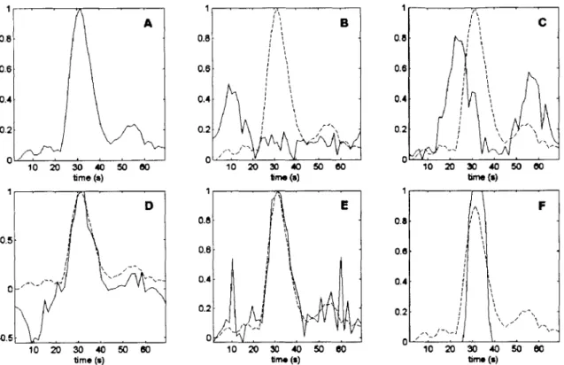
Figure 3.1.1: Examples of different AIs that would fail the exclusion criterion as compared to a given valid AIF. Plot A shows an idealized AIF with its single sharp peak and recirculation artifact. Plot B shows a potential AIF that violates properties 1 and 2 since it has an early first moment as well as an early peak, as compared to the ideal AIF. Plot C shows a potential AIF that violates property 3, since it has high concentration values that occur for longer than a typical bolus passage time. Plot D shows a potential

AIF that violates property 4, since the large negative peak is illogical and indicates noise

corruption. Plot E shows a potential AIF that violates properties 5 and 6 with the large concentration changes before and after the bolus. Plot F shows a potential AIF that violates property 7 since it does not have a recirculation peak, which is indicative of a motion artifact.

The second stage was the search stage, where the best AIF voxels were searched out and an AIF was determined for every voxel. This stage began by making a search cube of roughly (27mm)3 centered on each voxel in the brain. An example of the search cube size is shown in Figure 3.1.2. For each search cube, the corresponding criterions calculated earlier were normalized by subtracting out the minimum value of each statistic in the cube followed by dividing by the maximum value of each statistic in the cube. Thus, each criterion was constrained to between 0 and 1. Finally, these four criteria were converted into a score, S, defined to be:

S=FM-PV-AS+FWHM (3.1.1)

A

I . .

(22)

such that each voxel in the cube had a score between -2 and 2, with the ideal voxels having the lowest scores. The three voxels with the lowest score were then selected and interpolated with a 3-D 27mm FWHM Gaussian kernel. This result was stored as the AIF for the voxel centered in the cube.

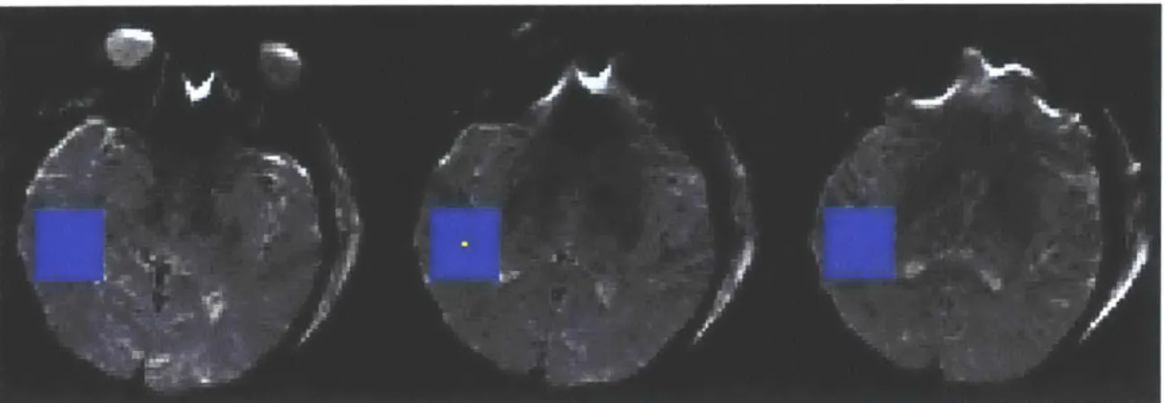
Figure 3.1.2 Example of the relative size of the (27mm)3 search cube (blue) for a given voxel (yellow) in the center image. The slices to the left and right of center are the slices above and below the center image, respectively. The resolution of the images is 1.72 mm2

with a slice thickness of 6mm and a gap between the slices of 1mm.

The final stage of the algorithm was the deconvolution stage which began by smoothing the local AIFs (for continuity) with the same 3-D Gaussian kernel used for interpolation. However, in order to prevent a bias on the edges of the brain, the AIF was extended out

by 14mm in all directions at the brain periphery in order to avoid edge effects during the

smoothing process. This was accomplished by adding extra slice above and below the brain, as well as using morphological operators to replicate the values on the edge of the brain out an extra 14mm. Finally, the local AIFs, Ca(t), were deconvolved from the concentration curves, C(t). The SVD approach described in Chapter 2 was used to do this deconvolution on a voxel by voxel basis. Following deconvolution, the MTT map was obtained by dividing the CBV map by the calculated CBF map. The entire local AIF algorithm, its stages and their important features are summarized in Figure 3.1.3 below. In addition, an implementation of the code using Matlab is given in Appendix B.

(23)

Signal Intensity Curves, Scanning Parameters

Calculate Baseline Intensity and Convert to Concentration

Calculate CBV

Exclude Corrupted Voxels

Calculate Voxel Statistics

Calculate the Score for All Voxels in the Search Cube

Interpolate the Three Lowest Scores and Store

Smooth with Gaussian Filter

Deconvolve Voxel by Voxel

Output

Figure 3.1.3 Flowchart Overview of the Local AIF algorithm

Define (27mm)3Search Cube

For Every Voxel in the Brain

Extend AIF on Edge of Brain

I Preparatory Stage Search Stage Deconvolution Stage -4 I I I

(24)

3.2 Example Outputs of the Local AIF Algorithm

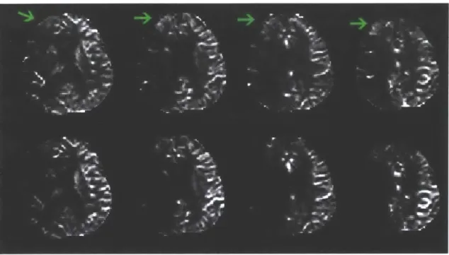
Figure 3.2.1 shows four CBF slices for a single patient that resulted from using the local

AIF algorithm (top row) as well as from using the standard global AIF algorithm (bottom

row). The local AIF algorithm is leading to flow increases in the ipsilateral hemisphere (i.e. the hemisphere of the brain which shows the perfusion defect). Particularly in the region pointed to by the green arrows, the local AIF algorithm is making a large difference.

Figure 3.2.1 Example CBF outputs for the local AIF (top row) and global AIF (bottom row) methods. The local AIF algorithm is increasing flow estimates in the ipsilateral hemisphere, as indicated with green arrows. Most likely, the decreased flow values on the global CBF are due to delay or dispersion of the contrast bolus.

Additionally, Figure 3.2.2 compares four MTT slices produced by the local AIF (top row) and global AIF (bottom row) methods. The local MTT is showing much less abnormality in the ipsilateral hemisphere, as indicated by the green arrows. The global MTT indicates that most of the ipsilateral hemisphere has an increased MTT, while the global method isolates it to a particular region. Thus, the local method appears to be more specific to the actual flow defect.

(25)

Figure 3.2.2 Example MTT outputs for the local AIF (top row) and global AIF (bottom

row) methods. As compared to the global MTT, the local MTT maps seem to be much more specific as to the actual region of flow defect. Particularly in the region indicated by the green arrows, the local AIF methods estimates a normal transit time, as opposed to the global method, which has nearly the entire ipsilateral hemisphere as abnormal.

3.3 Limitations of the Local AIF Algorithm

The beneficial effects of the local AIF algorithm are dependent on an uncorrupted dataset. As shown in Figure 3.3.1 below, the algorithm selects AIFs from all over the brain. Since it selects so many AIFs, such things as large patient motions (even after motion-correction), susceptibility artifacts or vessel pulsation can adversely affect the local AIF performance as they can lead to artificial signal drops which can cause regional discolorations in the perfusion maps in the areas where they are chosen as the AIF. This is because they lead to artificially high concentrations that lower the CBF estimate when they are deconvolved from the concentration-time curves. An example of the effect of patient motion is shown in Figure 3.3.2. In addition, a low contrast to noise ratio (CNR)

can also be detrimental to local AIF performance. The high noise variance can also lead to artificial signal drops, causing effects similar to those described above. Furthermore, the low contrast can make finding valid AlFs extremely difficult, particularly in regions

of low flow, which can occur in stroke.

(26)

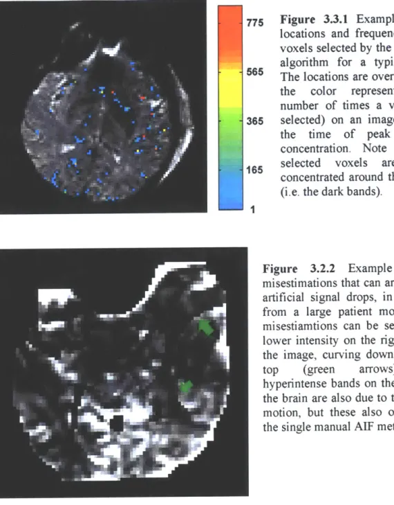
775 Figure 3.3.1 Example of the locations and frequency of the voxels selected by the local AIF algorithm for a typical slice.

565 The locations are overlaid (with the color representing the number of times a voxel was

365 selected) on an image slice at the time of peak contrast concentration. Note that the

165 selected voxels are highly concentrated around the vessels (i.e. the dark bands).

1

Figure 3.2.2 Example of the misestimations that can arise due to artificial signal drops, in this case from a large patient motion. The misestiamtions can be seen as the lower intensity on the right side of the image, curving down from the top (green arrows). The hyperintense bands on the edges of the brain are also due to the patient motion, but these also occur with the single manual AIF method

However, without care, auto or semi-automatic global AIF selection could choose a flawed AIF in any of these situations as well and produce worse perfusion metrics than the local approach since the error would not be isolated to a certain region of the brain. Thus, with the local AIF algorithm (and most automated techniques), scanner

(27)

3.4 Clinical Implementation

When converted to the C programming language, the local AIF algorithm can be used to calculate perfusion metrics for a 128x128x1 1x43 dataset in about 6 minutes on a 2GHz computer. Since an SVD must be calculated for every voxel in the brain, the

deconvolution accounts for roughly two thirds of the running time. Since most MRI scanners are programmed in a C derivative language that can run C programs, this would correspond to the running time on a recent MRI scanner. Unfortunately, six minutes is a long time to wait in a busy emergency room, although it is a significant improvement as compared to manual calculation. However, while this execution time may be slightly infeasible with current MRI systems, this execution time could easily be cut in half with either a dual processor system or faster CPU. Thus, with improved processing

(28)

(29)

Chapter 4: Effects of Using Localized AIFs

4.1 Introduction

The "gold-standard" technique for calculating perfusion metrics in animals is to inject microspheres into the bloodstream, euthanize the animal and then count the number of

spheres present in each volume of the brain. This technique, for obvious ethical reasons, is not an option in human perfusion research. Thus, without a "gold-standard"

quantitative technique for calculating in vivo perfusion metrics to compare directly, other techniques are needed to validate the performance of the local AIF algorithm. One way to

do this is to check that the new technique is actually fulfilling its potential. One of the important theoretical benefits of using local AIFs is that they should have a delay and dispersion that is approximately the same as the tissues near them. Thus, the local AIF algorithm should produce less flow misestimations due to delay and dispersion of the contrast bolus. Proving that the local AIF technique actually achieves this flow estimation improvement is then very important to the validation of the method.

We propose to validate the local AIF method by first examining its performance under normal and pathological conditions in clinical datasets. To accomplish this, CBF values

of the local and global AIF methods will be compared for normal and abnormal full width half max (FWHM) values as well as normal and abnormal time to peak (TTP)

values. Furthermore, the locations where large CBF ratios occurred will be mapped and compared. Finally, the average underlying tissue concentration curves will be calculated and compared for these large ratio voxels in order to understand where the method is making improvements.

4.2 Methods

4.2.1 Patient Selection

This study included 53 patients with diffusion and perfusion-weighted images obtained within the first 12 hours of symptom onset and a follow-up imaging on day 5 or later. The study population was selected from a retrospective database into which patients with ischemic stroke from 2 sites were registered between years 2000 and 2002. Fourteen of

(30)

the 53 patients were excluded because of motion or scanner artifacts. Three additional patients with completely normal PWI due to early reperfusion were also excluded. Of the remaining 36 patients, 21 were male and 15 were female. The mean age was 65 ranging from 26 to 83 years. There were 24 patients from site 1 and 12 patients from site 2. The cerebral infarction occurred within the territory of basilar artery in 1, posterior cerebral artery in 1, and middle cerebral artery in 34. The stroke mechanism was large vessel atherosclerosis in 10, cardiac embolism in 12, other rare causes in 4, small vessel disease in 1, and cryptogenic in 9 patients. The standard stroke treatment included anticoagulants and/or antiplatelet agents and no patients were treated by intravenous or intraarterial thrombolysis or experimental drugs.

4.2.2 MRI Acquisition

All data sets from site 1 were axial single-shot gradient-echo EPI images acquired during the first pass of 0.2 mmol/kg of a gadolinium-based contrast agent injected 10 s after the

start of imaging at a rate of 5 ml/s, followed by a comparable volume of normal saline injected at the same rate. These studies were performed on a 1.5 T General Electric

system with an MRI-compatible power injector (Medrad, Pittsburgh, PA). They had a

TR/TE = 1500/65 ms, a field of view (FOV) = 220 x 220 mm2_{, and an acquisition matrix}

= 128 x 128. The datasets consisted of 11 slices with a slice thickness of 6 mm and a gap of 1 mm, collected over 46 time points.

The data sets from site 2 were single-shot spin-echo EPI images obtained from a 1.5 T Siemens system with an MRI-compatible power injector (Spectris, Medrad, Pittsburgh,

PA). They had a TR/TE = 1200/78, an FOV of 26 x 26 cm2_{, and an acquisition matrix}

116 x 256 interpolated to 256 x 256. These studies contained 7 slices with a slice

thickness of 6.5mm and a gap of 1mm, collected over 40 time points. All data analysis

was performed retrospectively, with approval from our institution's committee for human subject research.

(31)

by first selecting a number of voxels from the MCA in the contralateral hemisphere of the brain and taking their average as the AIF for the entire dataset, as described in section 2.3. This AIF and the dataset were then run through a common SVD based deconvolution algorithm to create the global CBF maps. In addition, the local AIF algorithm described in Chapter 3 was used to create the local CBF maps.

4.2.4 CBF Difference Analysis

In addition to the CBF calculation, the FWHM and TTP of every voxel in the brain were also calculated in order to get a measure on the delay and dispersion of each voxel. The difference (Dig) of the local-defined CBF (lCBF) and the global CBF (gCBF) was then calculated for every voxel in the brain after normalizing by the average flow value in a normal gray matter ROI. The mean of the ratios for voxels with "normal" and delayed or dispersed TTP and FWHM voxels were then calculated on a patient by patient basis. More specifically, the "normal" TTP was defined to be one time point before the most frequent TTP found in the brain (TMF) and the "normal" FWHM was defined to be a one TR window centered on the most frequent FWHM (FmF). Furthermore, the "delayed" TTP was defined to be 4 time points after the "normal" TTP and the "dispersed" FWHM was defined to be a one TR window centered at 4.5 seconds after the "normal" FWHM. In summary, for each patient, we calculate:

TR TR pFn = mean (D g)FMF - < FWHM < FMF + (4.2.4.1) 2 2 TR T P Fd = mean (D g)|FMF +4.5- -< FWHM < FMF +4.5+ - (4.2.4.2) 2 2 prn = mean (Dig) TTP = TMF 1 (4.2.4.3) pTd = mean(Dig) TTP = TMF +3 (4.2.4.4)

Finally, for each patient the difference of these means were calculated for both TTP and FWHM. (i.e. pFd - pt]Fn and JTd -

ptTn-)-4.2.5 Voxel Location Analysis

Knowing where the ICBF values differ greatly from the gCBF values can also give us an indication of the benefits of the local AIF approach. To accomplish this, the mean and

(32)

standard deviation of both the ratio of ICBF and gCBF (Rig) and its inverse (Rgi, or the ratio of gCBF to ICBF) were calculated over the entire brain for each patient. Next, all voxels with an Rig greater than 1.75 standard deviations beyond the mean of Rig were found and their locations where highlighted on the CBF maps for that patient. Similarly, all voxels with an Rgi greater than 1.75 standard deviations beyond the mean of Rgi were found and highlighted in a similar manner. (For the rest of this work, having a ratio greater than 1.75 standard deviations beyond the mean will be considered a "significant difference"). Finally, the average tissue concentration curves for the voxels with a significant Rgi or Rig difference were calculated.

4.3 Results

4.3.1 CBF Difference Analysis

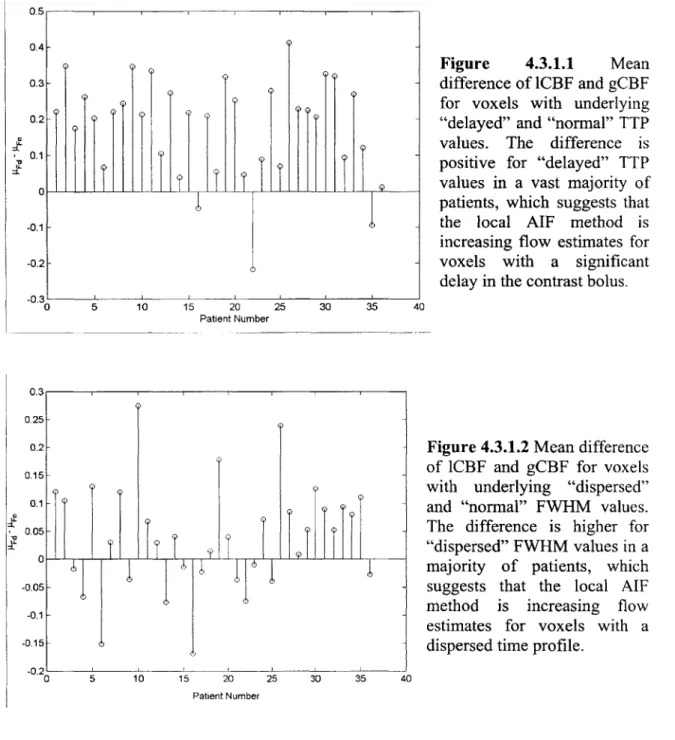
A stem plot of pITd - p-lTn is shown in Figure 4.3.1.1 on a patient-by-patient basis. In most

patients (31 out of 36), plTd, the mean difference of 1CBF and gCBF (i.e. Dig) with a delayed TTP is higher than IT, the mean of Dig with a TTP that is typical for the brain. This implies that the local AIF method is increasing flow values for voxels with a delayed tissue-concentration curve. It has been shown (9,11) that using an AIF that arrives too early compared to the underlying tissue-concentration can create flow underestimations. Thus, the local AIF method appears to be correcting these flow misestimations in most cases.

Similarly, a stem plot of ptFd - p-Fn is shown in Figure 4.3.1.2 on a patient-by-patient basis. In a majority of patients (23 out of 36), pFd, the mean of Dig with an increased FWHM, is higher than pFn the mean of Dig with a FWHM that is typical for the brain. It has also been shown (9) that dispersion of the concentration-time curves can also lead to flow underestimations. Thus, it appears that the local AIF method can correct these flow

(33)

0.4- 0.3-0.17 0 -0.1 -0.2--0.3 0 5 10 15 20 25 30 35 4 Patient Number 0.3 D.25 - 0.2- 0.15-0.1 0.05-n -0.05 -0.1 -0.15 -n .02

I

>1

5 10 15 20 25 30 35

ItI

Figure 4.3.1.1 Mean difference of lCBF and gCBF for voxels with underlying "delayed" and "normal" TTP values. The difference is positive for "delayed" TTP values in a vast majority of patients, which suggests that the local AIF method is increasing flow estimates for voxels with a significant delay in the contrast bolus. 0

Figure 4.3.1.2 Mean difference

of 1CBF and gCBF for voxels with underlying "dispersed" and "normal" FWHM values. The difference is higher for "dispersed" FWHM values in a majority of patients, which suggests that the local AIF method is increasing flow estimates for voxels with a dispersed time profile.

40 Patient Number

4.3.2 Voxel Location Analysis

Figure 4.3.2.1 below shows the difference of the percentage of total brain voxels

considered significantly different for Rig and Rgi. Thus, we see that for most patients, the local AIF algorithm is increasing flow values in more voxels than it is decreasing them. Accordingly, across all patients, the local AIF algorithm was significantly increasing

C

U. U.

=L

(34)

flow values for an average of 7.3% of voxels, while it was decreasing them for an average of 4.3% of voxels.

Figure 4.3.2.1 Percentage of voxels that the local AIF method significantly

increases flow estimates

minus the percentage of

voxels that the local AIF

method significantly

decreases flow estimates. For most patients, the local AIF method is leading to more

increased flow values.

0

5 10 15 20 25 30 35 40

Patient Number

Upon visual inspection of the voxel locations of significant 1CBF increase, it was found that in 7 of the 36 patients, the voxels were highly concentrated in the ipsilateral

hemisphere. For these same patients, there was no striking concentration of flow decrease in the ipsilateral hemisphere. An example of this phenomenon is shown in Figure 4.3.2.2, which shows blood flows with the locations of flow increase and decrease overlayed on all slices for one patient. Single slices from the remaining six patients with the same overlays are shown in Figure 4.3.2.3. In addition, there were 8 patients which had the locations of significant local flow increase concentrated in the ipsilateral hemisphere. However, these patients also had a high number of the local flow decrease voxels located in the ipsilateral hemisphere. Example slices from these patients are shown in Figure 4.3.2.4 with the significant voxel locations overlayed. Finally, there was one patient that only had a high concentration of significantly decreased local flow voxels in the

ipsilateral hemisphere. 0 0. lu 8 6 - C-4-o 0 -2- -4-

(35)

-6-Figure 4.3.2.2 Voxel locations of significant local CBF increase (blue) and decrease (green) for a single patient. Note the high concentration of the blue voxels in the ipsilateral hemisphere (the half of the brain that contains the lesion, indicated in red).

Figure 4.3.3.3 Example slices from patients with increased 1CBF voxels (blue) highly

concentrated in the ipsilateral hemisphere while the decreased 1CBF voxels (green) are not concentrated to a hemisphere. For reference, the follow-up lesion is indicated in red.

(36)

Figure 4.3.3.4 Example slices from patients with increased ICBF voxels (blue) highly

concentrated in the ipsilateral hemisphere but with a large number of the decreased 1CBF voxels (green) found in the ipsilateral hemisphere. For reference, the follow-up lesion is indicated in red.

When the average concentration-time curves were calculated for the increased 1CBF voxels, it was found that in 31 out of the 36 patients the underlying tissue curves had the

shape of a generalized concentration-time curve. On the other hand, only 13 out of the 36 patients exhibited a generalized shape for the decreased 1CBF voxels. These 13 were a subset of the 31 patients mentioned above, and they typically had a much lower

magnitude than the average curve for increased ICBF. Furthermore, when the 31 average curves with increased ICBF were compared to a typical AIF, it was found that they were delayed in 25 patients and dispersed in 17 patients with 16 patients exhibiting both delay and dispersion. A few examples of these average curves and the typical AIFs are plotted in Figure 4.3.2.5.

When these concentration-time curves were cross-referenced with the voxel location analysis described above, it was found that of the 8 patients with voxels of significant

(37)

Conversely, these patients had average concentration-time curves of lCBF decrease which were either very low magnitude or just noise. In addition, for the one patient which

showed the concentration of significantly lower 1CBF voxels in the ipsilateral hemisphere, it was found that this average tissue curve was just noise as well.

Furthermore, of the 7 patients that had the significant 1CBF increase voxels concentrated in the ipsilateral hemisphere with no concentration of 1CBF decrease voxels, 6 of these patients exhibited average underlying curves with the shape of generalized delayed or

dispersed concentration-time curves.

10 20 30 Dine (60=and6) 40 50 60 10 0.25 0.8 0.8 0-4 0.2 0.2 015 0.1 0.05 10 20 30 rum, (Seconds) 40 50 80 0.4 0.35 0.3 0.25 0.2 0.1 01 '0 10 20 30 Thme (secondS) 40 s0 n (6 1.4 1.2 1.0 0.8 0-6 0.4 0.4 0.351 0.3 0.25 0.2 0.15 0.1 0.05 0 10 20 30 Ten. (second.)

Figure 4.3.2.5 Examples of underlying tissue concentration-time curves and corresponding AIFs for two patients (arranged by row). Plots A and C show an AIF (solid line) compared to the average concentration-time curve for voxels with a significant 1CBF increase (dashed line) for two different patients. Note the delay of almost 6 seconds between the AIF and the average curves in both of these patients, as well as the widening of the curve (i.e. dispersion) in plot C. Similarly, plots B and D show the corresponding scaled AIF (solid line) as well as the average concentration-time curve for voxels with a significant 1CBF decrease (dashed line). Note the much lower magnitudes of the local flow decrease signals in both cases.

--- A 012 0.15 0.1 0.05 B 1.0 0.8 0.4 0.2 C

--

\

1.6 1.4 12 1.0 1 0.6 0.8 0.4 0.2 D - --40 50 s0 0

(38)

4.4 Discussion

We have shown that the local AIF method is capable of increasing flow estimates for voxels with underlying FWHM or TTP values which are delayed or dispersed. As was shown in Figure 4.3.1.1, for most patients, the flow estimates are increased for voxels with a longer underlying TTP. It must be noted that there are three cases which seem to not fit into this classification though. When the original raw perfusion data is examined however, the reasons for these contrary results are easily seen. In two cases, the region of perfusion abnormality is small, so nearly the entire brain sees no delay at all. In the other case, the contrast agent arrived normally to everywhere but the lesion, where it did not lead to a noticeable signal drop. Thus, in these three cases, there did not seem to be any considerable regions that could have been classified as having abnormal delay. Thus, the regions with these larger TTP values were probably noisy or nonsense voxels for which the flow ratios are erratic and unimportant.

Looking at the FWHM results in Figure 4.3.1.2, we see that the results are much noisier as compared to the TTP analysis, but the local AIF method still seems to be increasing the flow values in dispersed voxels on average. Upon examination of the four datasets yielding the lowest negative values in the plot, we see that similar phenomena to the TTP analysis above are influencing the FWHM calculation as well. The two patients with small lesions that led to contrary results in the TTP calculation also led to contrary results in the FWHM calculation, for most likely the same reason. With a small lesion, there was little to no dispersion, so the voxels with increased FWHM values were most likely noise. The other two patients were patients that seemed to not have been given quite enough contrast agent (i.e. had a low contrast to noise ratio, or CNR). Thus, the FWHM values could more easily be extended or shortened by the noise fluctuations and voxels that were not dispersed could be classified as dispersed, or voxels that were dispersed could be classified as not dispersed if a large noise fluctuation occurred at an opportune moment.

(39)

effect of the local AIF method on dispersed voxels should be attempted and this result should be taken only as provisional.

We also showed that the local AIF algorithm is creating significant flow increases in more patients than it is creating significant flow decreases (Figure 4.3.2.1). However, we see two outliers in this calculation as well. Upon inspection of these datasets, we find that one patient was not given enough contrast agent, while the other seems to have been given too much. The low CNR resulting from a deficit of contrast agent could make the local AIF calculation less accurate as it will be more difficult to find suitable voxels, and they could also be corrupted by noise. In addition, when too much contrast agent was used, the two methods disagreed on the flow voxels in or immediately near the large vessels. Since these values are so large, differences in these voxels are not really that important in terms of clinical diagnosis or treatment.

Furthermore, we showed that the voxels where the local AIF method was calculating significant ICBF increases were highly concentrated in the ipsilateral hemisphere in 15 patients (Figure 4.2.3.2-4). In addition, we looked at the average underlying

concentration-time curves for these voxels and found that in most cases, these were normal looking curves (albeit reduced) that often showed some measure of delay and/or dispersion (Figure 4.2.3.5). Of the 15 patients mentioned above, 12 patients had the generalized tissue curve shape, indicating that the flow improvement was on voxels that actually had some degree of flow in them. In some cases, the voxels of 1CBF decrease were also found in significant numbers in the ipsilateral hemisphere (Figure 4.3.4). However, in all of these cases, the average underlying curve for these voxels was either of negligible flow or was just noise. Thus, the ICBF decrease in these voxels appears to be insignificant, as these voxels are either nonsense or correspond to lesion tissue which has already infarcted. This seems to suggest that the groupings in Figure 4.3.3.3 and 4.3.3.4 were unnecessary as the decreased lCBF voxels in the ipsilateral hemisphere were mostly from dead or noisy tissue.

(40)

It must be noted however that there were a number of voxels for which the local AIF method increased flow estimates that still went on to infarction. While this is not necessarily a big problem, it certainly brings to light the question of this new method's

usefulness in clinical diagnosis. Thus, demonstrating that the changes to flow estimates that the local AIF method makes are clinically relevant is important to the validation of this technique, and is the topic of the next chapter.

4.5 Conclusions

The main theoretical benefit of using localized arterial input functions is that by using them, delay and dispersion of the contrast bolus are implicitly accounted for. In this work, by examining the voxels of significant flow differences between the local and global AIF methods as well as the average flow change for underlying levels of delay and dispersion, we have provided evidence that the local AIF method is actually increasing flow values for voxels which are delay and dispersed. Since it has been shown that delay and dispersion lead to flow underestimations, this suggests that the local AIF method is fulfilling its theoretical promise as a technique that is less sensitive to delay and

(41)

Chapter 5: General Linearized Model Analysis

5.1 Introduction

Chapter 4 showed that the local AIF method is making flow improvements in voxels with delay and dispersion, but the usefulness of this improvement was not explored. Since a "gold-standard" perfusion metric is unavailable, other methods of validation are needed. Since PWI is used largely in clinical situations for diagnosis or research post-stroke, another way to quantify performance is to compare how well the locally defined perfusion metrics can predict patient outcome as opposed to the older methods.

A general linearized model (GLM) is one way to do such an analysis (17). A GLM can

assign a tissue risk of infarction to every voxel in the brain, and these risk maps can then be cross referenced with follow-up scans of patient outcome to calculate statistics on the performance of the different techniques. These statistics can then be compiled into a receiver operating characteristic (ROC) curve and the performance of the different methods can be compared on the basis of their ROC curves. As an alternative, MTT lesion volumes can be outlined by an experienced neuroradiologist, and the results can also be cross-referenced to the follow-up lesion volumes. While this method may not be as sensitive since it is predominately based on only one imaging modality, it is at least a way to reinforce the results of the GLM by showing that the images obtained are useful to the human viewer and not just some mathematical model.

5.2 Methods

5.2.1 Patient Selection

This study included 53 patients with diffusion and perfusion-weighted images obtained within the first 12 hours of symptom onset and a follow-up imaging on day 5 or later. The study population was selected from a retrospective database into which patients with ischemic stroke from 2 sites were registered between years 2000 and 2002. Fourteen of the 53 patients were excluded because of motion or scanner artifacts. Three additional patients with completely normal PWI due to early reperfusion were also excluded. Of the remaining 36 patients, 21 were male and 15 were female. The mean age was 65 ranging

(42)

from 26 to 83 years. There were 24 patients from site 1 and 12 patients from site 2. The cerebral infarction occurred within the territory of basilar artery in 1, posterior cerebral artery in 1, and middle cerebral artery in 34. The stroke mechanism was large vessel atherosclerosis in 10, cardiac embolism in 12, other rare causes in 4, small vessel disease in 1, and cryptogenic in 9 patients. The standard stroke treatment included anticoagulants and/or antiplatelet agents and no patients were treated by intravenous or intraarterial thrombolysis or experimental drugs.

5.2.2 MRI Acquisition

All data sets from site 1 were axial single-shot gradient-echo EPI images acquired during

the first pass of 0.2 mmol/kg of a gadolinium-based contrast agent injected 10 s after the start of imaging at a rate of 5 ml/s, followed by a comparable volume of normal saline injected at the same rate. These studies were performed on a 1.5 T General Electric system with an MRI-compatible power injector (Medrad, Pittsburgh, PA). They had a TR/TE = 1500/65 ms, a field of view (FOV) = 220 x 220 mm2_{, and an acquisition matrix}

= 128 x 128. The datasets consisted of 11 slices with a slice thickness of 6 mm and a gap

of 1 mm, collected over 46 time points.

The data sets from site 2 were single-shot spin-echo EPI images obtained from a 1.5 T Siemens system with an MRI-compatible power injector (Spectris, Medrad, Pittsburgh, PA). They had a TR/TE = 1200/78, an FOV of 26 x 26 cm2_{, and an acquisition matrix =}

1 16x256 interpolated to 256 x 256. These studies contained 7 slices with a slice thickness of 6.5mm and a gap of 1mm, collected over 40 time points.

All 36 subjects also had EPI diffusion scans performed along with the perfusion studies.

Apparent diffusion coefficient (ADC), average diffusion-weighted images (DWI), and averaged non-diffusion-weighted images (LowB) maps were calculated from the diffusion data sets. All data analysis was performed retrospectively, with approval from

(43)

5.2.3 AIF Algorithms

For all patients, the global AIF perfusion maps were created by an experienced technician

by first selecting a number of voxels from the MCA in a single hemisphere of the brain

and taking their average as the AIF for the entire dataset, as described in section 2.3. This

AIF and the dataset were then run through a common SVD based deconvolution

algorithm to create CBV, CBF and MTT maps. These maps were created twice: once for AIFs selected from the ipsilateral and once from the contralateral hemisphere, with the maps resulting from the contralateral hemisphere considered as the globally defined perfusion metrics unless otherwise noted. In addition, the local AIF algorithm described

in Chapter 3 was used on all datasets, thus leaving three different sets of data to compare.

5.2.4 General Linearized Model

The GLM computed risk probabilities for every voxel using the following six parameters: LowB, ADC, DWI, CBV, CBF, and MTT in a method identical to that used by Wu, et al

(18). Just as in that work, the training of the model was accomplished via jackknifing (19). Jackknifing is a technique used to avoid the bias of running a model on the same

data that it was trained on. This is done by letting the model coefficients for each patient be those obtained by training the model on all of the other patients. Separate training and evaluation steps were performed for the global ipsilateral and contralateral AIF methods as well as the local AIF method, based on outlines drawn by an experienced

neuroradiologist.

These risk probabilities were then used to calculate the following statistics about the model's performance over the entire brain (based upon the above mentioned outlines): the true positives (TP, the number of voxels predicted to infarct that actually did); the false positives (FP, the number of voxels predicted to infarct which did not); the true negatives (TN, the number of voxels predicted to not infarct that did not infarct); and the false negatives (FN, the number of voxels predicted to not infarct that actually infarcted). From these statistics, the true positive ratio (TPR), or sensitivity, and the true negative ratio (TNR), or specificity, were calculated as: TPR=TP/(TP+FN) and

(44)

the false positive ratio (FPR, or 1 -specificity). Finally, the area under the curve (AUC), which has been shown to represent the probability that an image will be correctly ranked normal or abnormal (20), was calculated via trapezoidal integration. Statistical

comparison was performed by a Wilcoxon signed-rank test performed on the AUCs for each patient. Differences were deemed significant for p-values < 0.01.

5.2.5 MTT Lesion Volumes

Lesion volumes were outlined by an experienced neuroradiologist for the MTT maps generated by the contralateral, ipsilateral, and local AIF methods. These lesion volumes were then compared to the follow-up lesion volume and the mean squared error was calculated for the three methods. In addition, volumes were compared on a patient-by-patient basis with volumes classified as different only if they had a 20% volume disagreement. This was done in order to reduce bias associated with possible interexaminer dissagreement in the outlines.

5.3 Results 5.3.1 ROC Analysis

Figure 5.3.1.1A shows the ROC curves generated from running the multivariate GLM three times: once with each of the globally generated parameter sets and also with the locally generated set with only the CBF and MTT differing as input to the GLM. The local AIF approach has a higher ROC curve than either one of its global AIF

counterparts. Noticeably, the local AIF metrics show an increased sensitivity in areas of high specificity (FPR < 0.3) as compared to both of the global AIF metrics, while areas

of low specificity show a similar sensitivity. This means that in the region of high specificity, given an acceptable probability of incorrectly predicting that a tissue will infarct, the locally defined metrics will correctly predict a tissue to infarct with higher probability. This would make the local metrics preferable in the clinical setting, as it is preferable to not classify healthy tissue as unhealthy with high probability (particularly