Behavior of a coupled arch system

BEHAVIOR OF A COUPLED ARCH SYSTEM

by Tzu-Yang Yu

B.S. Department of Construction Engineering National Yunlin University of Science and Technology 1996

M.S. Department of Civil Engineering National Central University 1998

Submitted to the Department of Civil and Environmental Engineering in Partial Fulfillment of the Requirements for the Degree of

MASTER OF ENGINEERING IN CIVIL AND ENVIRONMENTAL ENGINEERING at the

MASSACHUSETTS INSTITUTE OF TECHNOLOGY June 2002

© 2002 Tzu-Yang Yu. All Rights Reserved.

The author hereby grants to MIT permission to reproduce and to distribute publicly paper and electronic copies of this thesis document in whole or in part.

Signature of Author:

Tzu-Yang Yu Department of Civil and Environmental Engineering May 10, 2002 Certified by:

Jerome J. Connor Professor, Department of Civil and Environmental Engineering

S-IF Thesis Supervisor

Accepted by:

MASSACHUSETTS INSTITUTE OFTECHNOLOGY

JUN 207

r 'Oral Buyukozturk

Chairman, Departmental Committee on Graduate Study

BEHAVIOR OF A COUPLED ARCH SYSTEM

Tzu-Yang Yu

Submitted to the Department of Civil and Environmental Engineering On May 15, 2002 in partial fulfillment of the requirements for the degree of

Master of Engineering in Civil and Environmental Engineering

Abstract

The arch is one of the most frequently used structures in civil engineering. By taking advantage of its shape, engineers can establish a system that allows the utilization

of the space below it. A space arch system has been proposed. It consists of two space parabolic arches leaning toward each other with brace members between them. A pair of leaning arches is more stable than a single arch because of the additional lateral stiffness due to the geometrical orientation. An investigation of the behavior is performed through numerical analysis using the finite element method (FEM). Several characteristic parameters are defined and investigated to find their influence on the load-carrying capacity of the system. The buckling behavior of the system is also discussed.

Keywords: Parabolic arch, pair of leaning arches, brace member, finite element method, buckling, stability.

Thesis Supervisor: Dr. Jerome J. Connor

Acknowledgements

I would like to express my gratitude to my advisor Professor Jerome J. Connor for his guidance and encouragement. Professor Connor is always available for questions and very dedicated to his students. His advice also inspires me on solving problems.

I would also like to thank Lisa Grebner for her useful suggestion to the thesis. I would like to thank many of my classmates for their warm and true friendship: Marc, Jason, Luca, Neeraj, Koji, and Chin-Huei.

Finally, I want to dedicate this thesis to my family and my girl friend, San-San. Their support and encouragement motivate my study at MIT.

Table of Contents

Sym bols and Abbreviations... 6

List of Figures ... 9

List of Tables ... 13

Chapter 1 Introduction

1.2 Scope ...-.. ... 19

Chapter 2 Literature Review

2.2 Analytical Solutions for Parabolic Arch Subject to Uniform Load... 22

2.3 Com parison of Different Form ulae for Arch Length ... 26

2.4 Critical Load of Single Plane Arch... 28

2.5 Critical Load of Braced Arches ... 30

2.6 Buckling M odes of Arches ... 32

2.7 A Pair of Leaning Arches System ... 33

Chapter 3 Methods of Analysis

3.1.1 Geom etrical Property ... 36

3.1.2 Boundary Conditions... 41

3.2 Loading Types ... 41

3.2.1 D istributed Vertical Load ... 41

3.2.2 Distributed Horizontal Load... 42

3.2.3 Concentrated Load ... 49

3.3 N um erical Approach... 50

3.3.1 Analytical, Experimental and Numerical Approaches ... 50

3.3.2 Finite Elem ent M ethod and Its Procedures ... 51

3.4 M aterial ... 52

Chapter 4 Analysis of A Coupled Arch System

4.3 Rise-to-Span R atio ... 58

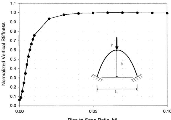
4.3.1 Vertical Stiffness... 59

4.3.1.1 Two-H inged Arch ... 59

4.3.1.2 Fixed Arch ... 60

4.3.1.3 D iscussion ... 61

4.3.2 H orizontal Stiffness ... 64

4.3.2.1 Tw o-H inged Arch ... 64

4.3.2.2 Fixed Arch ... 65

4.3.2.3 D iscussion ... :... 66

4.4 Leaning-to-D epth Ratio... 68

4.4.1 Vertical Stiffness... 69 4.4.2 H orizontal Stiffness... 70 4.4.3 D iscussion ... 71 4.5 Slenderness Ratio ... 74 4.6 Stability A nalysis... 76 4.6.1 In-Plane Buckling... 77 4.6.2 Out-of-Plane Buckling ... 83

4.7 D eform ation A nalysis... 87

4.7.1 Vertical Buckling ... 88

4.7.2 H orizontal Buckling ... 89

4.8 Structural Efficiency... 90

4.8.1 Structural Efficiency... 90

4.8.2 Variation of Internal Actions ... 93

Chapter

5

Conclusion

5.2 Suggestions...98

R eferences ...

100

Appendix

A .1 Plane Sim ple-Supported Beam ... 103

A .2 Plane Cantilever Beam ... 106

Symbols and Abbreviations

Symbols

a Distance of twin arch ribs

a _{Reciprocal of cc}

b _{Mean hourly wind speed factor}

b _{3-second gust speed factor}

A Area of cross section

Ao Total area of openings in a wall that receives positive external pressure, in ft2

Af Projected area normal to the wind except where Cf is specified for the actual surface area

Ag Gross area of that wall in which AO is identified, in ft2

c Turbulence intensity factor

Cf Net force coefficient

d Thickness at cross section of angle j from crown. do, dc Thickness of arch at crown

dk Thickness of arch at distance kL from crown

D Depth of the arch system

e Structural efficiency

E Young's modulus (modulus of elasticity)

h Rise of arch

gQ Peak factor for background response

gR Peak factor for resonant response

gV Peak factor for wind response

G Arch constant (Ch.2), Gust effect factor (Ch.3)

H, Ho Horizontal reaction

Hcr Critical intensity of the uniform load

I Moment of inertia at cross section of angle from crow (Except Ch.3)

I Importance factor (Ch.3)

Ic Moment of inertia of cross section at crown

IZ Intensity of turbulence

k Portion of position of load to entire span kN, kH Effective length factors

Kd Wind directionality factor

Kz Velocity pressure exposure coefficient

Kzt Topographic factor

1 Integral length scale factor

L Span of arch

Ld Leaning distance between two arches at crown

LT Reduced length of column

Lz Integral length scale of turbulence

MO Bending moment at support

mL, mR Bending moment on left and right half of arch, respectively

n Number of sections

Ncr,s Critical axial force at the quarter point of span length under symmetric loading Nx Axial force in an arch member

P Concentrated load

Pcr Buckling load of a column

q' Correction quantity due to geometry

qz Velocity pressure evaluated at height z of the centroid of area Af, lb/ft2

Q

QX

r Radius of gyration

R Resonant response factor

S Length of arch

t Change in temperature in degrees

V Basic wind speed

VO Vertical reaction

w, W Uniform load

wL Live load in pounds per square foot x, y, z Cartesian coordinates

Zg Nominal height of the atmospheric boundary layer zrnin Exposure constant

cc 3-second gust speed power law exponent

1

Xarch Arch analogy coefficient

p

one structure face for segment under consideration 0 Tilt angle of arch with respect to vertical plane

Ok Angle between tangent to arch-axis and horizontal

CTU Ultimate stress

Gy Yield stress

K Buckling coefficient

Slenderness ratio of arch

<p Angle of inclination of member's axis, at the considered section Angle from crown for circular arch

(D Reduction factor

Abbreviations

LTD Leaning-to-depth ratio

RTS Rise-to-span ratio

List of Figures

Gloucester Cathedral, Gloucester, England... 14

Ali Qapu (The Royal Palace), Isfahan, Iran ... 14

Roman Amphitheater, Nimes, France ... 15

Temple Guiting Church, Gloucestershire, England... 15

Arc de Triomphe, Paris, France... ₁₅

Cloaca Maxima, Rome, Italy... ₁₆

The mouth of the section of the Cloaca Maxima across from S. Giorgio in Velabro, Italy... 16

The temple of Hercules Victor by Giovanni Battista Piranesi (in mid 1800 A.D.) about Cloaca Maxima, Rome, Italy... 16

Pont du Gard, Nimes, France ... 17

Ang-Ji Bridge, Her-Pei, China ... 17

Pont d'Avignon (Bridge of Saint Benezet), Avignon, France ... 17

Principle of load transfer ... 18

Actions between arch members... 18

Illustration of the system... 20

Comparison of Different Formulae ... 27

Distribution of Load ... 29

Typical Models used by Sakimoto et al... 31

Symmetric Buckling ... 32

Anti-Symmetric Buckling ... 32

Asymmetric Buckling... ₃₃

Illustration of the model ... 34

Top view of the model... ₃₄

Side view of the model... ₃₄

A typical pair of leaning arches system... 36

A parabola... _{. . 37}

Plot of Melan's Equation ... 38

Front view of the system (x-z plane)... 38 Figure 1.8 Figure Figure Figure Figure Figure Figure 1.9 1.10 1.11 1.12 1.13 1.14 Figure 2.1 Figure 2.2 Figure 2.3 Figure 2.4 Figure 2.5 Figure 2.6 Figure 2.7 Figure 2.8 Figure 2.9 Figure 3.1 Figure 3.2 Figure 3.3 Figure 3.4

Figure 3.5 Figure 3.6 Figure 3.7 Figure 3.8 Figure 3.9 Figure 3.10 Figure 3.11 Figure 3.12 Figure 3.13 Figure 3.14 Figure 4.1 Figure 4.2 Figure 4.3 Figure 4.4 Figure 4.5 Figure 4.6 Figure 4.7 Figure 4.8 Figure 4.9 Figure 4.10 Figure 4.11 Figure 4.12 Figure 4.13 Figure 4.14 Figure 4.15 Figure 4.16 Figure 4.17 Figure 4.18 Figure 4.19 Figure 4.20 Figure 4.21

Top view of the system (x-y plane)... 39

R ise-to-Span ratio, h/L ... 39

Depth-to-Leaning ratio, Ld/D ... 40

Distribution of dead load of parabolic arch... 42

B asic W ind Speed... 44

Definition of Variables used for Topographic Factor, Kt ... 45

Side Projection of the System ... 48

Distribution of Air Current (Top View)... 49

Different types of arch bridge ... 50

Typical Stress-Strain Curve for Metal... 53

Arch-Column Analogy ... 56

Arch Analogy Coefficient and Rise-to-Span Ratio (Two-Hinged Arch).. 56

Arch Analogy Coefficient and Rise-to-Span Ratio (Fixed Arch)...57

Rise-to-Span Ratio vs. Vertical Stiffness (Two-Hinged Arch) ... 59

Rise-to-Span Ratio vs. Vertical Stiffness (Enlarged) ... 60

Rise-to-Span Ratio vs. Vertical Stiffness (Fixed Arch)... 60

Rise-to-Span Ratio vs. Vertical Stiffness (Enlarged) ... 61

Vertical Stiffness Ratio, kfixed/khinged ... 62

Vertical Stiffness Ratio (Enlarged)... 62

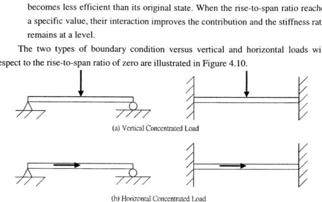
Different Loads and Different Boundary Conditions (RTS Ratio = 0).... 64

Rise-to-Span Ratio vs. Horizontal Stiffness (Two-Hinged Arch)... 64

Rise-to-Span Ratio vs. Horizontal Stiffness (Enlarged between 0 and 0.1) 65 Rise-to-Span Ratio vs. Horizontal Stiffness (Fixed Arch)...65

Rise-to-Span Ratio vs. Horizontal Stiffness (Enlarged)... 66

Horizontal Stiffness Ratio, kfixed/khinged ... ---... 67

Horizontal Stiffness Ratio (Enlarged between 0 and 0.05) ... 67

Leaning-to-Depth Ratio and Tilt Angle...68

B raced range... 69

Leaning-to-Depth Ratio vs. Vertical Stiffness... 69

Leaning-to-Depth Ratio vs. In-Plane Horizontal Stiffness...70

Figure Figure Figure Figure Figure Figure Figure Figure Figure Figure 4.22 4.23 4.24 4.25 4.26 4.27 4.28 4.29 4.30 4.31 Figure 4.32 Figure 4.33 Figure 4.34 Figure 4.35 Figure 4.36 Figure 4.37 Figure Figure 4.38 4.39 Figure 4.40 Figure 4.41 Figure 4.42

Numbering of Brace Members ... 71 Variation of Axial Forces in Brace Members (Vertical Load)...72 Variation of Axial Forces in Brace Members (In-Plane Horizontal Load) ... 73 Slenderness Ratio and Vertical Stiffness ... 74 Slenderness Ratio and In-Plane Horizontal Stiffness...75 Elastic Buckling Load Parameter (By Austin and Ross, 1976)... 77 Elastic Buckling Horizontal Reaction Coefficient (By Austin and Ross,

1976) ... 7 8 In-Plane Sym. Concentrated Buckling Load vs. Radius of Gyration.. 78 In-Plane Sym. Uniform Buckling Load vs. Radius of Gyration ... 79 In-Plane Sym. Concentrated Buckling Load vs. Stiffness Ratio of

B race to A rch... 79 In-Plane Sym. Uniform Buckling Load vs. Stiffness Ratio of Brace to A rch ... . . 80 In-Plane AntiSym. Concentrated Buckling Load vs. Radius of

G yration ... . . 8 1 In-Plane AntiSym. Uniform Buckling Load vs. Radius of Gyration .. 81 In-Plane AntiSym. Concentrated Buckling Load vs. Horizontal

W ind L oad ... 82 In-Plane AntiSym. Uniform Buckling Load vs. Horizontal Wind

L oad ... . 82 Out-of-Plane Sym. Concentrated Buckling Load vs. Radius of

G yration ... . . 83 Out-of-Plane Sym. Uniform Buckling Load vs. Radius of Gyration.. 84 Out-of-Plane Sym. Concentrated Buckling Load vs. Stiffness Ratio of B race to A rch ... 84 Out-of-Plane Sym. Uniform Buckling Load vs. Stiffness Ratio of B race to A rch ... 85 Out-of-Plane Sym. Concentrated Buckling Load vs. Horizontal

W ind L oad ... 85 Out-of-Plane Sym. Uniform Buckling Load vs. Radius of Gyration.. 86

Figure 4.43 Figure 4.44 Figure 4.45 Figure 4.46 Figure 4.47 Figure Figure Figure Figure Figure 4.48 4.49 4.50 4.51 5.1 Figure A.1 Figure A.2 Figure A.3 Figure A.4 Figure B.1 Figure B.2 Figure B.3 Figure B.4 Figure B.5 Figure B.6 Figure B.7

Design Chart for Vertical Dimensionless Displacement Ratio and

Slenderness R atio ... 88

Design Chart for Horizontal Dimensionless Displacement Ratio and Slenderness R atio ... 89

Structural Efficiency for Vertical Stiffness (Two-Hinged Arch) ... 91

Structural Efficiency for Vertical Stiffness (Fixed Arch)... 91

Structural Efficiency for Horizontal Stiffness (Two-Hinged Arch)...92

Structural Efficiency for Horizontal Stiffness (Fixed Arch)... 92

Variation of Axial Force and RTS Ratio... 93

Variation of Bending Moment and RTS Ratio ... 94

Variation of Shear Force and RTS Ratio ... 94

Stiffness versus LTD Ratio... 97

A plane simple-supported beam-Point Load... A plane simple-supported beam-Uniform Load ... A plane cantilever beam- Point Load... 103 105 106 A plane cantilever beam-Uniform Load ... 107 D efinition of m om ent of inertia ...

Rectangular cross section ... Circular cross section ... D esign cross section -- Section A ...

D esign cross section -- Section B ...

D esign cross section -- Section C ...

Tube cross section ...

109 110 111 111 112 112 113

List of Tables

Table 2.1 Buckling coefficient K given by Stussi (1935)... 28

Table 3.1 Mechanical properties of steel (E. Mizuno, 1997)... 52

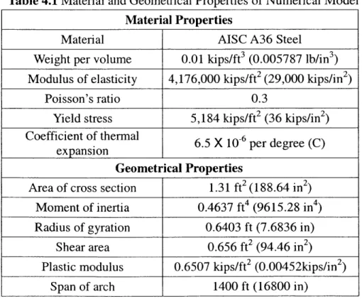
Table 4.1 Material and geometrical properties of numerical model... 58

Chapter 1 Introduction

1.1 Overview

The arch is one of the oldest forms of architecture and civil engineering. After the appearance of the first prototype of arch about 5000 years ago in Middle-East area (Ur, Bagdad) it seems that the mechanical efficiency of arch has been noticed and applied by ancient people, even though they did not understand its principles.

In architecture, the application of arch is focused on connection between two columns and the support of the roof above. Many ancient religious buildings displayed the characteristic aesthetic appeal of the arch on their exterior (Figures 1.1, 1.2, 1.3, 1.4, and 1.5). Nevertheless, the importance of the arch had been demonstrated even before its appearance in civil engineering applications (Figures 1.6, 1.7, and 1.8), especially on bridges (Figures 1.9, 1.10, and 1.11).

Figure 1.1 Gloucester Cathedral, Gloucester, England (-A.D.1953)

Figure 1.3 Roman Amphitheater, Nimes, France (A.D. 100-A.D.200)(left) Figure 1.4 Temple Guiting Church, Gloucestershire, England (A.D. 1873)(right)

Figure 1.6 Cloaca Maxima, Rome, Italy (About B.C.600)

Figure 1.7 The mouth of the section of the Cloaca Maxima across from S. Giorgio in Velabro, Italy (B.C.100)

Figure 1.8 The temple of Hercules Victor by Giovanni Battista Piranesi (in mid 1800 A.D.) about Cloaca Maxima, Rome, Italy (About B.C.600)

Figure 1.9 Pont du Gard, Nimes, France (B.C.19)

Figure 1.10 Ang-Ji Bridge, Her-Pei, China (A.D.605)

What ancient people knew about the arch mechanism might be that, by arranging members properly, the loading could be "guided" through members toward supports (Load Transfer) (Figure 1.12). With the aid of frictional action induced by compression between members, space would be gained below the arch (Figure 1.13).

[7

77

Jr

/

Figure 1.12 Principle of Load Transfer

F/ / / / /

-I

UlllililU

t

The applications of arches in bridges are more challenging than for buildings. This is because the required span of a bridge is usually large and the reserved space below the bridge is necessary for other uses. However, the applications of arches in bridges display their advantages thoroughly. Materials were the limitation of the development of arch bridges in ancient times. It was not until the emerging of new materials, such as reinforced concrete, that the spans of arch bridges could be promoted to new level.

Arches can be categorized into many types, depending on the following factors: 1) Geometrical property: a) Shape: Circular, parabolic, hyperbolic, etc.

b) Boundary condition: Fixed, hinged, etc. c) Global Configuration: Two-dimensional or

three-dimensional. d) Internal Configuration: Continuous or hinged. 2) Physical property: a) Material: Reinforced concrete, steel, stone, etc.

b) Mechanics (Load-carrying mechanism): Carries load from top of it (through compression member, such as pillar or truss) or carries load below it (through tension member,

such as hanging cable).

When designing an arch system, the following factors should be mentioned and considered with respect to the design requirements. The choice of arch type depends on:

1) Purpose of arch 2) Structural efficiency 3) Construction feasibility 4) Terrain and geology

5) Aesthetics

6) Economics (Cost) 7) Maintenance

1.2 Scope

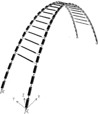
The arch system to be considered in this thesis is a pair of leaning parabolic arches, connecting to each other with bracing member between them (Figure 1.14). It is a three-dimensional structure because it takes load and offers stiffness in three dimensions. The systems is capable of carrying loads from hanging cables attached to it and from pillars above, so as to behave like an arch bridge or an arch structure.

Commercial software is used for establishing numerical model and performing parametric analysis (SAP2000, Computers and Structures Inc., 1998).

Figure 1.14 Illustration of the system

This thesis is organized in the following manner. First, the review of previous research on the topic of arch is given. Next, the configuration of arch system and description of analysis method are introduced. Finally, a pair of leaning parabolic arches is examined and investigated through parametric analysis. Stiffness and stability analyses

Chapter 2 Literature Review

All theories are evolved from empirical form to analytical form, not excepting the theory of the arch. The advancement of a theory usually depends on the discovery of new phenomena and the invention of new tools for analysis.

2.1 Overview

The development of the arch theory began with geometry and then looked into mechanics. Bolarch (1755) published a book containing architectural design examples of arches. Swan (1794) introduced the work done by architects and offered design scenarios. Atwood (1801) published a dissertation on the material properties or behavioral properties of arches. Lagarrigue (1831) investigated arch geometry and pointed out that the tilt angle of an arch might be a characteristic design parameter. Nicholson (1851) collected many design examples and displayed empirical formulae based on different construction materials. Swain (1896) compared the analysis theories for different structures and mentioned the stress analysis of arch.

Melan (1915) published a book and introduced the analytical method and graphical method for arches, considering different types of boundary condition and loads. He proposed a graphical method and used the concept of influence-lines to determine the dimension of arch sections.

Timoshenko (1934) introduced the classical approach from the former Soviet Union for establishing and solving mechanical problem analytically. His several famous books on mechanics provided following researchers a clear way to obtain a universal solution.

MIT Professor Spofford (1937) described his experience with designing arch bridges in his book. He dealt with the design of continuous arch bridges of different shapes and presented analytical solutions with numerical verification.

Leontovich (1959) published a book collecting analytical solutions of arches of different shapes and considering different types of loading and boundary condition. His work provided designers a short path on evaluating the design by internal action and reaction. Leliavsky's (1982) work considered the detailed designs of components of arch

bridge. He mentioned many practical issues including long-term effect in his book.

Most of the previous works followed an analytical approach and encountered many difficulties. The main reason is geometry. When the shape of structure is irregular and can not be described by continuous mathematical function, it is not easy to formulate the relation between variables because they are geometrically dependent.

There are several ways to amend the weakness of an analytical approach. One can simplify the geometry such that the description is feasible. The disadvantage becomes the error induced by oversimplification. Or one can analogize a describable structure to the complicated structure by establishing the relationship between them. However, this strategy still requires further verification by other approach, usually numerical methods.

The goals of analysis are: i) Stiffness

i) Critical load (Buckling load) ii) Internal actions

iii) Deformation

Analysis is complete once the information listed above is obtained. Several analytical results for a plane parabolic arch with different boundary conditions are presented in the following sections.

2.2

_{Analytical Solutions for Parabolic Arch Subject to Uniform Load}

Melan (1915) offered his analytical solution by graphical method for two-hinged parabolic arch subject to uniform load distributed along the projection of its entire length on horizontal axis: LMb y ds H= I fds+ I r A _(2-1) 1 1wL2 Mb=--wx(L-x)- _y 2 8 f

4f

where H = horizontal reaction; L = span of arch; Mb = bending moment in a simple beam; f = height (rise) of arch; I = moment of inertia of section; w = uniform load; x, y =

coordinates of arch-axis; V = coordinate of the center of curvature of the arch-axis; r =

radius of curvature of arch-axis at any section (only defined here); A = area of cross section. If the arch is symmetrical, the vertical reactions at two supports are half of the total load and equal to each other. In fact, Eq.(2-2) is equivalent to standard parabolic function. Its derivation is in Chapter 3.

For fixed end parabolic arch subject to uniform load,

Mbyds -Vq

H=I r

L 2_{ds +}y dx

I r A

(2-3) where q' = correction quantity due to geometry.

Melan also mentioned the method to determine the thickness of arch from the concept of line of resistance. In order to generate same vertical projection of section, the thickness is defined as

d = do sec

#

where do = thickness at crown; d = thickness at cross section of angle

4

where n = number of sections.

Melan's graphical method contains many simplifications and definitions. His method involves the concept of line of resistance and influence. It is only applicable in the elastic

range. Some of the simplifications may induce significant error when the rise-to-span ratio (or height-to-span) of arch is large.

Spofford (1937) provided another formula for uniform load over entire structure: 1 hwL2

H=15 EIC

1 8 h2

AE 15 EIC

(2-5)

where H = horizontal reaction; h = rise of arch; w = uniform load; L = span of arch; EIL = rigidity of arch; - = coefficient of thermal deformation; t = change in temperature in degrees; A = area of cross section.

For two-hinged parabolic arch subject to concentrated load,

PhQLJ)(k _{4 -2k} 3 +k) ±etE H 3 IC H = 1 8 h2 A 15 I (2-6) where P = concentrated load; k = portion of position of load to entire span. For fixed end arch subject to any loading,

H =. I I 0 2 y2 I A E = ML + R 2 x2 I 1 +EmR+ 2 1 (2-7) where HO = horizontal reaction; VO = vertical reaction; MO = bending moment at support. mL, mR = bending moment on left and right half of arch, respectively, due to applied loads, considering each half of arch to act as a cantilever fixed at left and right ends; I = moment of inertia of section.

Spofford defined the thickness of cross section in the manner of moment of inertia for two-hinged parabolic arch:

I =-I. sec

#

28 ec~/5(2-8)

where I = moment of inertia at cross section of angle

f

For fixed end arch, the thickness is determined as

dk = d c4l+tan2 _(2-9)

where dk = thickness at distance kL from crown; dc = thickness at crown; Ok = angle

between tangent to arch-axis and horizontal. dc is determined as dc .F + +WL +

10 200 400 _(2-10)

where L = span of arch; wL = live load in pounds per square foot (50 percent to be added for impact on railroad bridge); w, = weight of fill over crown in pounds per square foot. F.W. Weld gave this relation in 1905. Obviously it is an empirical expression.

Similar restraint applies to the formula in Professor Spofford's book, which is applicable for flat arches with small rise-to-span ratio.

Leontovich (1959) published a book collecting condensed solutions for different types of arches and frames. For vertical uniform load over entire span of two-hinged parabolic arch,

H =WL

8f

(2-11) where H = horizontal reaction; w = uniform load; L = span of arch; f = rise of arch. The axial force in arch is computed by

L 1 X x!-->Nx =H cosV+jw sin V 2 (2 L+ x>2 _{->N,=Hcos±p+w X sinV} 2 _{(L 2)} (2-12) where x = horizontal distance from support; Nx = axial force in an arch member, acting at the section defined by the horizontal coordinate x; p = angle between tangent to

arch-axis and horizontal.

For vertical uniform load over entire span of fixed end parabolic arch,

H =wL

8f (1+ G) _(2-13)

where G is a arch constant, defined by d12

G =1.5

(2-14) where dj.₅ = _{arch thickness at crown (in proper dimensional units); t} = numerical constant. Shear force is also calculated by

L I X

x ->

Q,

2 2 L

L I X

x>-o>Qx= _{H sinpo+w 2-LCos 0}

s

(2-15) where

Qx

distance x.

The way Leontovich determined the thickness of arch is d=dgsc

d sec = d (2 -16 )

where p = _{angle of inclination of member's axis, at the considered section.}

Leontovich derived the expression of reaction and internal action from the aspect of force equilibrium. When static indeterminate structure was encountered, he integrated simplified coefficient into the expression. Other cases of different loading conditions and types of boundary condition could be referred in his book. His systematic work is helpful for evaluation of preliminary design.

2.3 Comparison of Different Formulae for Arch Length

The length of arch is essential for determining gravity load, which is the self-weight of member. When preliminary design is proceeding, a handy formula is required for evaluation with sufficient precision.

parabolic arch. It is shown as below:

S =L 1+ 1h

S=L 3± j<(2-17)

where S = length of arch.; L = span of arch; h = rise of arch. This formula was obtained by neglecting some higher terms during integration.

Leontovich (1959) offered another formula.

L 4h 2 L lg4h 4h2

S =-- 1lg-+ + 1+7 -~

2 1L

s=r

-~.k

iC K]}(2-18)

Definitions are the same with Eq.(2-17).

Their comparison with numerical solution is shown in Figure 2.1.

400 350 300 V) C, 0 -j 250 200

Length of Parabolic Arch (L = 100 ft)

150

I-0 0.1 0.2 0.3 0.4 0.5 0.6 0.7 0.8 0.9

Rise-To-Span Ratio

Figure 2.1 Comparison of Different Formulae

It is found that Eq.(2-17) is applicable to flat arch (rise-to-span ratio < 0.3) and not applicable when rise-to-span ratio is greater than 0.4. The difference between Eq.(2-18) and numerical solution is undetectable. Hence, when flat arch is designed, Spofford's formula is recommended. When stocky arch is designed, Leontovich's formula is recommended.

Continuous Line = Numerical Solution

Triangle Mark = Spofford's Formula

Circle Mark = Leontovich's Formula

2.4 Critical Load of Single Plane Arch

Komatsu and Shinke (1977) proposed their formula for determining the ultimate strength of a plane arch subject to symmetrical loading.

a 1 > Ns = Ao-y (1-0.136a-0.3a2 a>1> Ncrs = A 12 Y\.773+a _(2-20) And -- 1 L a=-E r (2-21) where Nr,s = critical axial force at the quarter point of span length under symmetric loading; A = average cross-sectional area; ay = yield stress; K = Buckling coefficient given by Stussi (1935); E = Young's modulus; h = rise of arch; L = span of arch; r = radius of gyration about horizontal centroidal axis of arch cross-section.

Table 2.1 Buckling coefficient K given by Stussi (1935) Type _Rise-to-Span Ratio, h/L

0.1 0.15 0.2 0.3

Two-hinged arch 36.0 32.0 28.0 20.0

Wv

H H

(a.) Symmetric Load

P

1-I ', I 111 11,111 11 11 T 111[ IT P I I I I

L

(1) UnsymmetriC Load

Figure 2.2 Distribution of Load

For asymmetric loading, Komatsu (1985) modified the formula by Stussi and provided his formula:

Ncr =DNcrs _(2-22)

where D = reduction factor. It is computed by

(D=I- C -W C C1 +C2 h E C, =2.2-+0.018 -- 0.19 L _, - 2 - L _-J E 0-C2K= -4K --r6K x;2

K

where W = uniform loading over entire span of arch; P = uniform loading over half span of arch.

Sakimoto (1997) offered a formula derived from elastic linear theory for a parabolic arch subjected to uniform load and non-uniform load (Figure 2.2(b)).

The critical horizontal reaction is computed through the following formula:

Hc = " 1+- _{-- P)}

"r 8h _ 2 W- _(2-24)

in which Hr = critical intensity of the uniform load. If define ac, as Hcr divided by A and divide Eq.(2-24) by 7y, then it becomes

0a w, L2F1(P >1

07_r -cr 1+1 I

o-, _{8hAo-, _ 2 W ) (2-25)}

where P = 0 in the case of an uniform distributed load.

Sakimoto (1997) also mentioned the effect of slenderness ratio, defined as Ijr, on the critical stress. The critical stress increases as the slenderness ratio decreases, which means increasing the size of cross section or decreasing the span of arch can increase corresponding critical stress.

2.5

Critical Load of Braced Arches

Sakimoto, Yamao and Komatsu (1979) provided their formula based on the results of theoretical and experimental investigation for estimating ultimate stress 7u, subjected only to vertical loads.

auU( _y

N= =Ao-( _2-26)

where cy = yield stress; Nu = ultimate axial force at springings of arch rib; A = average cross-sectional area.

a =1-0.136A, -0.3Z,2 _:A~ =1.276-0.888y+0.1762 e 1 s I, s 2.52 - 1 a- =- -> 2.52 1A, y7 _(2-27) And

- 1 c-, KL

AV

K=KeKflKI

Ke= 0.5 =>fixed; Ke= 1.0 => hinged

2r

Kea

K, =0.65 -> hanger -loaded; K, = 1.0 m vertical - loaded _(2-28)

where K = effective length factor; ry = radius of gyration about vertical centroidal axis of arch cross section; a = distance of twin arch ribs;

p

W - p L

A

A

1,

I

I

I,

Figure 2.3 Typical Models used by Sakimoto et al. (1979)

HT

.1

I

I

/

I

VVVVV

AA/\AA

2.6 Buckling Modes of Arches

When the load acting on an arch increases, the arch loses its stability once a certain critical value of the load is attained. In the case of elastic structures under conservative loads, the critical load corresponds to a stability limit point or a bifurcation point. When the arch configuration and the loading conditions are symmetric with respect to the crown of arch, the equilibrium path bifurcates from the original deformation mode to the buckling deformation mode. When the buckling deformation occurs in the plane of arch, it is called in-plane buckling. When it occurs out of the arch plane, it is called out-of-plane buckling.

The buckling modes are symmetric (Figure 2.4), anti-symmetric (Figure 2.5) and asymmetric (Figure 2.6). The onset of which mode depends on the type of arch.

Figure 2.4 Symmetric Buckling

Figure 2.6 Asymmetric Buckling

In Figures 2.4 and 2.5, _{the concentrated load is applied at the center of arch. In Figure}

2.6, the load is not applied at the canter of arch. For the in-plane problem of two-hinged arch or a stocky arch, an anti-symmetric buckling occurs under the smaller load. For the out-of-plane problem in these cases, a symmetric buckling occurs under smaller load. In the case of an asymmetric arch or a symmetric arch subjected to an asymmetric load, the load and deformation increase simultaneously until the maximum or limit load is reached.(Sakimoto and Komatsu, 1982)

2.7 A Pair of Leaning Arches System

Sakimoto et al.(1982) reported an investigation on an arch bridge system. Their arch bridge is consisted of two arches in parallel, connected with bracing system between two arches. Nevertheless, their arches are vertical, which means perpendicular to the ground (or bridge slab).

Plaut et al.(1998) performed research of a pair of leaning arches. They discussed the deflection shape, vibration modes, and the stability of a system of a pair of leaning arches. Molly et al.(1999) carried out similar research using the same model but subject to different loads. Their model consisted of two tilting arches leaning with each other. In their model, tilting angle is an essential factor for their research. However, their model does not involve bracing system between two arches. Their two arches connect with each other only at crown point.

other and connected with a bracing system between two arches. The tilt angle and bracing system are parameters in this research. The model is illustrated in Figures 2.7, 2.8 and 2.9.

Figure 2.7 Illustration of Model

Figure 2.8 Top View of Model

Chapter 3 Methods of Analysis

3.1 Description of System

The behavior of an arch depends on two main parameters: geometrical configuration and loading condition. If an arch extends on three axes in space and is subjected to loading from any direction, its behavior is three-dimensional. If an arch can be described on a plane and is only subjected to loading on the plane, its behavior is two-dimensional. If an arch is configured on a plane but subjected to out-of-plane loading, its behavior is still three-dimensional.

Single arches possess inherent instability. It is because a single arch can only provide its out-of-plane stiffness through the bending rigidity from its supports. Once it loses its bending rigidity at support, it becomes unstable. Single arch with two-hinged support is also unstable out of plane.

A coupled arch system improves the weakness of single arch through its three-dimensional configuration. The coupled arch system discussed in this thesis is defined as "a system consisted of two arches leaning together with tilt angle and connected with bracing member between them." A coupled arch system achieves its stability by using bracing member between two arches. The main constraint to the system is whether the support should be fixed-type or the connection (between brace and arch) should be fixed-type. Another way for the system to attain its stability is to make the brace become a truss. More bracing members are required to form atruss system in that case. In this thesis, the connection between bracing member and two arches is assumed to be fixed-type, and the supports to be two-hinged-type and fixed-type.

The concept of a pair of leaning arches is an inherently stable system. Two arches, inclined toward each other in the direction perpendicular to their arch planes and connecting with another through bracing member, possess the capacity of resisting load from any direction. The illustration of such a system is shown in Figure 3.1.

Figure 3.1 A typical pair of leaning arches system

3.1.1 Geometrical Property

The system can be defined through geometrical description. Once the shape of arch is chosen according to some regular configuration, the geometry can be determined by mathematical equation. In this paper, the shape is determnined by parabolic equation.

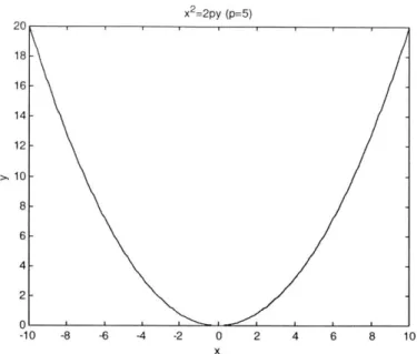
Several standard equations of the parabola are given in Cartesian coordinate.

(a)x2 = 2py

2x

(b)y2 = 2px

Wc)(y -k )2 =2p(x-h)

(d)

(x

(y

where x, y are ordinates on x-axis and y-axis, respectively; p, k, and h are all coefficients. Plot of (a) is illustrated in Figure 3.2.

The form of parabola in Polar coordinate is

r =1

1- cos 6 (3-2)

70

60

50

0 10 20 30 40 50 60 70 80 90 100

Figure 3.2 A parabola

Melan (1915) gave an equation for determining the His equation is derived from standard parabolic equation, the following calculation. Its form is

y=4f I-XI

L T

relationship between x and y. which can be proved through

(3-3) In Eq.(3-3), L = span of arch, f = rise of arch, x and y = coordinates of axes. Note that the origin is at left and of the member. It yields to

y=4f 4f )> y =- x2_ f L L) _L L _ o-y= 4fx2 -2 (Lxz: ->- y 2X2-2 (Lx+(L) L! 2 xf 2 L2 L 2 1---(y-f)= x-- -> =--=2(-L 4f ₂

_(y

Comparing to (d) in Eq.(3-1), they are identical when h = L/2, k = f, p =-L 2/(8f).

Leontovich's Equation -- y=4f(1-x/L)(x/L), f=70, L=100

40

10

30

x2=2py (p=5) 20 18- 16- 14- 12-> 10 - 8- 6- 4- 2-0 -10 -8 -6 -4 -2 0 2 4 6 8 10 x

Figure 3.3 Plot of Melan's equation

Using Eq.(3-3), one can determine the coordinates on x and y axes.

The coordinate on z-axis can be defined either by a linear or nonlinear distribution. When linearly distributed on x-z plane, it means that there are two straight lines connecting the crown and two supports. When nonlinearly distributed, the lines connecting the crown and two supports are two curves. In this paper, only linearly distributed coordinate on x-z plane is considered. The front view of the system is illustrated in Figure 3.4.

HF f4

Plane view is also rendered in Figure 3.5.

Figure 3.5 _{Top view of the system (x-y plane)}

In order to describe the system, several geometrical parameters are defined and introduced below:

(1) Rise-to-Span Ratio, h/L

The characteristic of parabolic arch in height can be represented in terms of rise-to-span ratio, h/L. _{The higher the arch, the larger the ratio.}

h

L

Figure 3.6 Rise-to-Span ratio, h/L

(2) Depth-to-Leaning Ratio, Ld/D

Depth-to-leaning ratio, Ld/D, is defined to be the ratio of the distance between two arches at crown to the distance at support. When Ld/D is zero, two arches are connected with each other at crown without distance. When Ld/D is unity, the lateral projection of the system will look like a typical frame with vertical columns.

Ld

Figure 3.7 Depth-to-Leaning ratio, Ld/D

(3) Slenderness Ratio, L/r

Similar to the definition of slenderness ratio in columns, L is the span and r is the gyration radius of cross section. It is computed through Eq.(3-5).

L _L

=L

r Fa I

r II(

3 -5 )

where Ia is the moment of inertia of cross section, Aa is the area of cross section. Using the linear distribution, the coordinate on z-axis can be computed through Eq.(3-6) and (3-7). Define the arch on the right side in Figure 3.7 to be the first arch, the left to be the second, therefore,

FirstArch>z=- _D-L (3 n 2 (3-6) SecondArch -> zi = D n 2 _(3-7)

where zi is the coordinate on z-axis, i is the index of the coordinate starting from the support and n is half the number of total segments of an arch. An arch is simulated by 20 straight segments (n=10).

3.1.2 Boundary Conditions

Two types of boundary conditions are considered; fixed and hinged. It is not allowed to generate any displacement at support in both cases. There will be rotation in hinged case. The boundary conditions in terms of displacement and reaction are expressed in Eq.(3-8) - (3-11).

Displacement

Fixed Support

ujI =0;u, =0;uj =0

A31 KU =0; fly SU = 0; /3z fSU = 0 _(3-8)

Hinged Support

u2, =0;u = 0;uI = 0

6IS 0;#; P # 0I(3 9) Reaction Fixed Support F, F 0;YF F Y 0;F 0 M, #0;2 M, 0;ZM~ 0 (3-10) Hinged Support IF, # 0;jXF, #0; Fz # 0 MX =0; jM, =0;ZMz =0 _(3-11)

3.2 Loading Types

3.2.1 Distributed Vertical Load

The type of distributed vertical load corresponds to the weight of structure. It includes any fixed member or attached equipment, which will affect the long-term behavior of structure. Since distributed vertical load is induced by gravity and proportional to the volume of structure, the estimation of loading becomes the calculation of the volume of structure. The nature of gravity load is static, according to Newton's laws of motion, when there is no relative motion between the internal center of gravity

and the external reference axis. For this reason, gravity load is also called dead load. Because of the configuration of arch, the distribution of dead load is not linear with respect to the span of arch. The distribution of dead load of parabolic arch is shown in Figure 3.8. The length of arch can be computed by Eq.(2-18) or by summing up the length of each segment.

Distribution of Dead Load 3

S2.5--

2-

1-5--10 -8 -6 0 6 8 10

Distance (from center, L=20m)

Figure 3.8 Distribution of dead load of parabolic arch (Normalized to the value at center)

3.2.2 Distributed Horizontal Load

The type of distributed horizontal load corresponds to the pressure exerted by wind, which is called wind load. The estimation of wind loads follows the regulation by American Society of Civil Engineers (ASCE) 7-98. Three allowable methods are provided in ASCE 7-98. They are (1) Method One -Simplified Procedure; (2) Method Two - Analytical Procedure; and (3) Method Three - Wind Tunnel Procedure. Method Two is adopted in this thesis.

Design wind loads are functions of wind velocity, wind direction, terrain, exposure, structural system and exterior of system. The arch system can be considered as a frame having all walls open. This leads the arch system fall in the category of open building, which is defined as "a building having each wall at least 80% open."(Sec. 6.2, ASCE 7-98) In other words,

A0 0.8Ag _(3-12)

pressure, in ft2_{;A9 = the gross area of that wall in which AO is identified, in ft}2_.

Design wind force, F (lb), on open buildings and other structures is:

F = qzGC A _(3-13)

where q, = velocity pressure evaluated at height z of the centroid of area Af, lb/ft2 G = gust effect factor; Cf = net force coefficient and Af = projected area normal to the wind except where Cf is specified for the actual surface area.

Velocity pressure, qz, at height z can be computed by Eq.(3-14).

qz =0.00256KZKztKdV2_{I (3-14)}

where K, = velocity pressure exposure coefficient; Kt = topographic factor; Kd = wind directionality factor; V = basic wind speed (Figure 3.9); I = importance factor.

According to the definition of exposure category, assume the location of the arch system belongs to "urban and suburban areas", which is Exposure B. By assuming Exposure B, corresponding constants are used in Eq.(3-15).

a =7.0; z =1200(ft); = ;b= -;

7 7

1-a =-;b =0.45; c =0.3;l = 320(ft);zen = 30(ft)

4 _(3-15)

where a = 3-second gust speed power law exponent; zg = nominal height of the atmospheric boundary layer; a = reciprocal of ; b = 3-second gust speed factor; a

= mean hourly wind speed power law exponent; b = mean hourly wind speed factor; c

= turbulence intensity factor; 1 = integral length scale factor; zmin = exposure constant. For 15 ft < z < zg, K, = 2.01(z/zg)2". At the top of arch, z = 233 ft. Thus, K, = 1.258.

From the table given by ASCE 7-98,

(233-200

Kh = _{(1.28 -1.20)+1.20 =1.2528}

(250-200 . _(3-16)

For topographic factor, Kzt,

, 90(40) 100(45) T \ 110(49) 120(54) 130(58) 140(63) 130(58) 140(63) 140(63) 14,0(63) _150(67) 150(67) Special Wind Region

90(40) 100(45) 130(58) Location _{V mph (mis)} 110(49) 120(54) Hawaii _{105 (47)} Puerto Rico 145 (65) Guam 170 (76) Virgin Islands 145 (65) American Samoa 125 (56) Notes:

1. Values are nominal design 3-second gust wind speeds in miles per hour (m/s) at 33 ft (10 m) above ground for Exposure C category.

2. Linear interpolation between wind contours is permitted.

3. Islands and coastal areas outside the last contour shall use the last wind speed contour of the coastal area.

4. Mountainous terrain, gorges, ocean promontories, and special wind regions shall be examined for unusual wind conditions.

where K =0.95;y=4;p=1.5 K2 =1 Ix PuLh -Yz K3 = e 4

Definition of Lh, x and z is shown in Figure 3.10.

v(z) x(Upwind) Lh V(Z) SI 7 rlecd-U~p ,nwind) HW2 H/2 X 7/7 ,/ .7 7/'

Figure 3.10 Definition of Variables used for Topographic Factor, Kt

Assume H/Lh = 0.5, x/Lh = 0.0 and z/Lh = 1.165, such that K1 multiplier = 0.53, K2

multiplier = 1.00, K3 multiplier = (1.165-1)/(1.5-1)*0.02 = 0.0066. Then,

K, =0.95;,y = 4;u p=1.5 K2 =1- 0 =1 1.5x 200 K₃ -4x233 e 200 = 0.0095 > K1 -

[1+(0.53

z

(3-18)

k

Recall Eq.(3-14), to compute qz

qZ = 0.00256KZKZtKd V2I

--> qz = 0.00256 x1.258 x1.000063 x 0.85 x 110 2

x1.0

-> q, = 33.1247(lb / ft2) _(3-20)

For gust effect factor, G, use the following formula:

_+.7 g Q 2+g2R2

Gf =0.925

r

1+1.7gI,

(3-21) in which Iz = intensity of turbulence; gQ = peak factor for background response; gR = peak

factor for resonant response; g, = peak factor for wind response. gQ and g, shall be taken as 3.4. The background response

Q

1

Q

1+0.63 B+h

(O -hjj(3-22)_{6 3} r

in which B = horizontal dimension of structure measured normal to wind direction (ft); h = height of a structure. L, = integral length scale of turbulence. The choice of the magnitude of B of the arch system is not easy to determine because the arch system is not a solid building with regular shape. The diameter of arch member is 5 ft, which means 10-ft width to be the width of obstacle for wind. Therefore, B is taken to be 10 ft.

Z

= 33 _(3-23)

Substituting given constants, L, becomes

I- = 320 =509.247(ft) 33 (3-24) And 1 Q = ,a 0.8828 1+0.63 10+133 0.82 509.247) _(3-25)

R = I RRRB (0.53 +0.471R) where R, =7.47N (1+1.3N)N/ 3 N,= 33) 60) (3-26) r> 0->R,=I- (1-e-2n 77 272 77=-> R, =1 _(3-27)

where the subscript I in Eq.(3-27) shall be taken as h, B, and L respectively. That means R, = Rh-> 7n= 4.6 R 1(1 V-Z

q

-0.45 x 133 0.25 (33) x11Ox 88 = 102.87 60 0.3376 x 133 = 2.0078 - R,,= 0.3763 q = 4.6x 102.87 7 = 4.6x 0.3376xl =0.15 1 RB= 0.9065 102.87 77= 4.6x 0.3376 x10 = 0.151 RL = 0.9065 102.87 _(3-29)

Here B = L =10 ft and N = 1.6713 as calculated. Thus, R,, = 0.099. Assume damping ratio for each mode is 2% = 0.02, R equals to 0.3092.

33 //6 33 6

I, = c -I =0.3-x = 0.2378 (3-30)

Kz 133 (-0

Peak factor for wind response is calculated by

0.577 S n(3600) 21n(3600n) -> 2ln

(3600x0.3376)

For force coefficient factor, Cf, the formula is

Cf = 4.0e2 -5.9e+4.0

(3-32) where , = ratio of solid area to gross area of one structure face for segment under consideration. Take side projection of the arch system (Figure 3.12), compute the value of

F to be 2231.4 / 7354.94 = 0.3034. Because there is some overlap at upper bracing

members and the round shape of arch, take E to be 0.25 would still be conservative.

294 ft

24,64 ft

246 ti _{25.6 ft}

+ t

r 332.92

Therefore, force coefficient factor Cf is computed to be 2.775. And finally, design wind load is to be 147582.63 lb = 147.583 kips.

The reduction of round shape from rectangle is because of the distribution of air current and the effect of vortex. The air current distribution is displayed in Figure 3.12.

Vortex D

ArchQ

Figure 3.12 Distribution of Air Current (Top View)

If wind comes from the direction perpendicular to arch axis, different force coefficient factor (Cf = 3.61) is used and results in another wind load.

F = 33.1247 x 0.894x 3.79x 899 =101508.81(lb) _(3-33)

The application of horizontal distributed load will induce the problem of stability. This part is discussed in Chapter 4.

3.2.3 Concentrated Load

Concentrated loads are applied to the system when cables are hang below it or when pillars are supported above it. The application of hanging cables is usually for supporting a bridge slab (for through type arch bridge) or elevated structure. Pillars are used when arch is used in deck type arch bridge. Different types of bridge are shown in Figure 3.13. The magnitude of concentrated load is assumed to be constant and the result

of stiffness analysis will be normalized to obtain a dimensionless relationship between variables.

(b) Half-through type arch bridge

(a) Through yXe arch bridge

Figure 3.13 Different types of arch bridge

3.3 Numerical Approach

There are many available approaches to be used for research. They can be categorized into three main types: analytical, experimental and numerical. Their pros and cons are briefly discussed in the following section.

3.3.1 Analytical, Experimental and Numerical Approaches

The advantage of using analytical approach is its universality. Once governing equation is established and solved, an analytical answer is applicable to different cases of the same characteristics. Meanwhile, an analytical solution offers us the relationship between different variables. We can even derive some symbolic index for evaluating the response. The disadvantage of an analytical approach is establishing the model physically and solving the equation mathematically.

Another way is the experimental approach, which can be performed in model size (model test) or real size (full-scaled test). Nevertheless, experimental approach is