ASPECTS OF BIOLOGICAL SEQUENCE COMPARISON
by
Stephen Frank Altschul B.A., Harvard College (1979)
Submitted to the Department of Mathematics in partial fulfillment of the requirements for the degree of
Doctor of Philosophy at the
Massachusetts Institute of Technology June, 1987
(D
Stephen F. Altschul, 1987The author hereby grants to M.I.T. permission to reproduce and to distribute copies of this thesis document in whole or in part.
Signature of Author
Signature Redacted
I Certified by Accepted by Department of Mathematics -- ebruar- 12, 1987
Signature Redacted
7
D~aniel J.0 Klgytman7is 10rvisor
Signature Redacted
Accepted byProf. Willem V. R. Malkus Chairman, Applied Math Committee
Signature Redacted
Pkof. Sigurdur Helgason
Chairman, Departmental Graduate Committee
MASSACHUSET ITUE Department of Mathematics
OF TECHNOL Y
TABLE OF CONTENTS DEDICATION...4 ABSTRACT...5 ACKNOWLEDGEMENTS...6 I. INTRODUCTION... Biological sequences... Sequence transformation... Sequence alignment.... ... ... The cost of an alignment... A brief history of biological sequence comparison... Outline of the thesis... II. BASIC TERMINOLOGY AND METHODS... Path graphs... Dynamic programming... III. OPTIMAL SEQUENCE ALIGNMENT USING AFFINE GAP COSTS...
Affine path graphs...
An alignment algorithm for affine gap costs... Comments on the SS-2 algorithm... Previous algorithms... A biological example... ... Concave gap costs... Conclusion... 10
11
... . . 13 .. . . .. . . 15 .17.17
.19
... 21 ... . .22...
30
.... . .
33
...
37
...
39
.. .. .. .
43
.. .. .. .
46
IV. SUBALIGNMENT SIMILARITY FUNCTIONS... Probabilistic similarity function s ... Interpolation of function s... Analytic function s2... Other similarity functions... V. ALGORITHMS FOR FINDING LOCALLY OPTIMAL SUBALI
Gap costs...
Locally optimal subalignments... The SIM subroutine... Comments on the SIM subroutine.... The LES subroutine... Comments on the LES subroutine.... The TT-2 algorithm... The NES-1 subroutine... Comments on the NES-1 subroutine.. The VV-1 algorithm... The NES-2 subroutine... Comments on the NES-2 subroutine.. Weak local optimality... ...
GNMENTS....
Isosimilarity curves and the feasible region..
...47 ... 49
.51
... 54.55
.56
.56
.58
.59.60
.61
.62.63
.63
.64
.65
.65
.67.68
... .... .... .... .72 ... ... 0 ...The DD algorithm... Comments on the DD algorithm... Self-optimality... A test for self-optimality... A relative prefilter: the RPF subroutine.... Comments on the RPF subroutine... An absolute prefilter: the APF subroutine... Comments on the APF subroutine... The CC pattern recognition algorithms... The CC-1 algorithm... Comments on the CC-1 algorithm... The CC-2 algorithm... Implementation of the CC-1 algorithm...
VI. SIMILARITY SIGNIFICANCE LEVELS... Range of the analysis... Estimation of parameters... Nucleic acid sequences with non-uniform nucleotide Protein sequences.... ... Hypothesis testing... Generalizations... Three-sequence comparison... .76
.79
.81 ... 82 ...83
.85 ...85 ...89
... 92 ... 92 ... 95 ... 95 .. 95 .. 100 .. 102 .. 103 ..106 .. 121 .. 125 .. 127 .. 127 .. 131 .. 131.. 136
usage.. .. 0 . . .. . .0 .. 0 . . .. 0 . . VII. APPLICATIONS... Comparison of interleukin 2 cDNA... Comparison of yeast and E. coli pyrophosphatases... APPENDIX. RANDOM DINUCLEOTIDE AND CODON PRESERVING SEQUENCE PERMUTATION.142 Terminology... 143Graphs and edge orderings...146
Random DP premutation algorithm...152
DNA examples...153
Random doublet and triplet preserving permutation...154
Random doublet and triplon preserving permutation...154
Random DtP permutation algorithm...156
A DNA example...157
Significance of an interferon alignment...159
For
Stephan R. Wagner
ASPECTS OF BIOLOGICAL SEQUENCE COMPARISON by
Stephen Frank Altschul
Submitted to the Department of Mathematics
on February 12, 1987 in partial fulfillment of the requirements for the degree of Doctor of Philosophy in Mathematics.
ABSTRACT
This thesis investigates methods for finding optimal alignments and subalignments of biological sequences and assessing their statistical
significance. Specifically, nonlinear similarity functions are proposed as the most appropriate for comparing subalignments, in contrast to the linear similarity functions in wide use. Algorithms are developed for finding locally optimal subalignments, using any reasonable similarity function as a selection criterion. The statistical significance of nucleic acid and protein sequence subalignments is investigated using Monte Carlo methods. The methods developed are used to find interesting alignments from several real biological sequences. In addition, the thesis identifies and corrects mistakes in the literature concerning the optimal alignment of two
sequences using affine gap costs, the time complexity of finding optimal alignments using concave gap costs, and the random permutation of a sequence preserving its doublet frequency.
ACKNOWLEDGEMENTS
First, I wish to thank Professor Bruce Erickson for his encouragement, time, ideas and advice over two and a half years. Without his help this thesis could not have been written.
I am indebted to Professors Peter Sellers and Joel Cohen for many useful suggestions and for providing me with space and resources with which
to complete this work.
I am grateful also to Professor Bruce Merrifield for allowing me to join his laboratory at the Rockefeller University.
I am appreciative of financial support from various institutions, namely the National Science Foundation, which supported me with a Graduate Fellowship; the Mathematics Department, which supported me with teaching assistantships; and the Office of Naval Research and the Army Research Office which supported me through a research contract with Professor Bruce Erickson.
Finally, I would like to thank Professor Peter Sellers and the members of my thesis committee, Professors Daniel Kleitman, Bruce Erickson and Mike Sipser, for their criticism of the manuscript of this thesis.
I. INTRODUCTION
A sequence is a finite string of letters drawn from a finite alphabet. While a sequence may be treated as a purely abstract entity, many sequences have their origin in the real world. Examples of real-world sequences are pieces of English text and sequences representing the primary structure of biological macromolecules, such as proteins or nucleic acids. The set of questions it is fruitful to ask about real-world sequences depends upon the origin of the sequences. The questions investigated in this thesis are some of those that seem appropriate for protein or nucleic acid sequences. Since the discussion will be abstract, the results will apply to sequences of any kind.
Biological sequences. Deoxyribonucleic acids (DNA), ribonucleic acids (RNA) and protein molecules are each constructed as a linear sequence of a small set of chemical building blocks. (In some cases the DNA sequence is circular.) DNA molecules generally are double stranded with each strand composed of four types of deoxyribonucleotide in a specific order. The two strands of a DNA molecule are complementary so that the sequence of
nucleotides in one strand determine the sequence of nucleotides in the other. RNA molecules generally are single stranded, with a strand
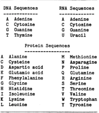
constructed from four types of ribonucleotide. Protein molecules consist of one or more polypeptide chains constructed from twenty types of amino acid. The building blocks of DNA, RNA and protein molecules frequently are represented by single letters from the Latin alphabet, as shown in
Table 1-1. One letter codes for DNA, RNA and protein sequences
DNA Sequences A Adenine C Cytosine G Guanine T Thymine RNA Sequences A Adenine C Cytosine G Guanine U Uracil Protein Sequences Alanine Cysteine Aspartic acid Glutamic acid Phenylalanine Glycine Histidine Isoleucine Lysine Leucine M N P
Q
R S T V w y Methionine Asparagine Proline Glutamine Arginine Serine Threonine Valine Tryptophan Tyrosine A C D E F G H I K LThe primary biological function of a DNA molecule is carrying genetic information encoded in the sequence of its nucleotides. It is reasonable that much of the relevant information about a DNA molecule can be captured in an abstract sequence from an alphabet of four letters representing the four deoxyribonucleotides. In contrast, the biological function of many RNA and all protein molecules is dependent upon their conformation in
space. It is thought that under physiological conditions this conformation is strongly dependent upon the sequence of building blocks from which the molecules are constructed. Predicting the three-dimensional structure of
these molecules from their sequences alone remains a distant goal.
Nevertheless, much information can be gleaned from protein sequence data. For example, two proteins with similar sequences may be evolutionarily related or may share a similar three-dimensional structure. We shall be content to represent RNA and protein as well as DNA molecules by abstract sequences of letters (Table 1-1).
Sequence transformation. Consider the three sequences "SHEHERAZADE", "SHEVARDNADZE" and "IGLOO" drawn from the space of sequences of letters of the Latin alphabet. Intuitively, the first two sequences are closer or more similar to one another than either is to the third. One approach to formalizing this concept is to define a set of operators on the space of sequences. For example, one operator might change the letter "A" to the letter "B"; a second might delete the letter "X"; a third might reverse the order of any two adjacent letters. A sufficiently rich set of operators will allow any sequence in the space to be transformed into any other by repeated use of the operators. If a positive cost is assigned to each
operator, then the cost of a given transformation of one sequence into another can be defined as the sum of the costs of the operators employed. The distance between two sequences can be defined as the minimum cost for transforming one into the other. Generally operators are defined so that if a given operator will transform sequence X to sequence Y, the inverse operator exists and has the same cost. When this is the case, distance as defined above behaves as a metric on the space of sequences.
Real-world considerations may affect the choice of operators and the costs assigned to them. For example, one may hope to correct spelling errors in typed text by finding the nearest neighbor(s) of an unrecognized word. A reasonable operator to use in such a context might be one that allowed two adjacent letters to be transposed. The cost of replacing one
letter by another might be related to the physical distance of two letters on a keyboard. For errors made in electronic text transfer a totally different set of operators and costs would probably be desirable.
Sequence alignment. The theory of evolution provides the main justification for comparing biological sequences. Two proteins with the same function in different species may have evolved from the same ancestral protein; two sections of DNA in the same gene may have descended from a duplicated ancestral fragment. There are mechanisms of mutation that
permit the substitution of one nucleotide for another and the deletion or insertion of one or more nucleotides. These mutations at the DNA level can appear at the protein level as substitutions, deletions or insertions.
While more complicated mutations are possible, these three types are the most common.
When the only operators permitted are those that substitute one letter for another and those that delete or insert one or more letters, a natural object of study that is central to this thesis is a sequence alignment. An alignment of two sequences is a one-to-one ordered correspondence of their elements, where an arbitrary number of nulls (missing letters) may be inserted into each sequence. Two nulls may not be placed into
correspondence. One alignment of "SHEHERAZADE" and "SHEVARDNADZE" is SHE-HER--A-ZADE
SHEV-ARDNADZ--E
There is no simple correspondence between sequence transformations, as described above, and sequence alignments. For example, a transformation of
"SHEHERAZADE" to "SHEVARDNADZE" may pass through the sequence
"THEHERAZADE". There is no way of indicating this in an alignment.
Both sequence transformations and sequence alignments can be thought of as explaining relationships between sequences. Alignments promote parsimony of explanation. A letter of one sequence is either unaltered, changed into a different letter, or deleted. More roundabout explanations of relationship are excluded.
In this thesis, a subsequence of a sequence is a string of adjacent letters from the sequence. A subalignment of two sequences is an alignment of a subsequence from each sequence. A diagonal (sub)alignment is a
(sub)alignment containing no nulls.
The cost of an alignment. As with sequence transformations, the intuition that one sequence alignment is better (more convincing as an
explanation of relationship) than another is formalized by defining a
real-valued cost function on alignments. While an infinite variety of cost functions can be imagined, we use the operator notion to narrow the
definition.
DEFINITION. A substitution cost function is a real-valued function on unordered pairs of letters.
DEFINITION. A gap cost function is a real-valued function on strings of letters.
DEFINITION. Given substitution and gap costs, the cost of an
alignment or subalignment is the sum of the substitution cost for each pair of aligned letters and the gap cost for each maximal string of letters aligned with nulls.
In this thesis, we shall assume that alignments with lower cost are better and that all costs are rational and non-negative. Further, we shall assume that the gap cost of the concatenated string XY is never greater
than the sum of the gap costs of the individual strings X and Y. For
purposes of illustration we shall frequently use the substitution cost
function cid(xy) defined to be 0 when x = y and 1 otherwise.
In the literature of biological sequence comparison, alignment cost as defined above has sometimes been called distance or similarity (Needleman and Wunsch, 1970). We shall use the word distance to mean the minimum cost of aligning two sequences and shall reserve the word similarity for a
constraints to those given above are either implied or explicitly imposed on the substitution and gap cost functions. For instance, Sellers
(1974a,b) places conditions on substitution and gap cost functions that force the minimum cost of aligning two sequences to act as a metric on the space of sequences.
A brief history of biological sequence comparison. The method of dynamic programming (described below) was introduced to biological sequence comparison by Needleman and Wunsch (1970) to find optimal alignments of two protein sequences. Their algorithm had time complexity O(MN), where M is the length of the shorter and N the length of the longer sequence. Though they speculated on the possibility of using various substitution and gap costs, they.confined their study to the case in which all gap costs are identical. Sankoff (1972) described how the dynamic programming approach could be modified so that only alignments with fewer than a fixed number of gaps were studied. Sellers (1974a), treating the null element as a member of the alphabet, proved that if the substitution costs provide a metric for the alphabet, then this metric can be extended to the space of sequences. He also showed (Sellers, 1974b) that a dynamic programming algorithm can be used to find the distance between any two sequences. Waterman et al.
(1976) described an algorithm of time complexity O(MN2
) for finding the optimal alignments of two sequences when arbitrary gap costs are allowed. This contrasted with Sellers' algorithm, which required the gap cost of a string to be the sum of the gap costs for each element of the string.
Dayhoff et al. (1978) derived a substitution cost function for protein sequence comparison from studies of related proteins with known sequences.
Schwartz and Dayhoff (1978) studied the relative effectiveness of this and other substitution cost functions for detecting distant relationships among proteins. Smith and Waterman (1981a,b) proposed that Needleman-Wunsch similarity can be used to define optimal subalignments for two sequences, and described an algorithm for finding optimal subalignments. Smith et al.
(1981) showed that the Sellers minimum-cost and the Needleman-Wunsch maximum-similarity definitions of optimal alignments are equivalent.
Gotoh (1982) described an O(MN) time algorithm for finding an optimal alignment of two sequences when affine gap costs are used. His paper was only partly correct (Chapter III; Altschul and Erickson, 1986a) since his algorithm correctly finds the minimum alignment cost but in general does
not produce an alignment that has this cost. Sankoff and Kruskal (1983) edited a book reviewing the entire field of sequence comparison, in which Erickson and Sellers (1983) described an algorithm for finding optimal alignments of a specified sequence with unspecified subsequences of a second sequence. Fitch and Smith (1983) showed that affine gap costs may be necessary to find the biologically correct alignment of two sequences.
Fitch (1983a) described a procedure for permuting a sequence while preserving its doublet frequency. His conjecture that this procedure generates with equal probability all sequences that have identical doublet
composition is incorrect (Appendix; Altschul and Erickson, 1985). Ukkonen (1983) described an algorithm for finding the optimal alignment of two sequences which in most cases runs much faster than the traditional dynamic programming algorithm. Waterman (1984a) reviewed the field of sequence comparison.
Waterman (1984b) described two algorithms for finding the optimal alignment cost of two sequences when arbitrary concave gap costs are
allowed. He conjectured that these algorithms have time complexity O(MN). This conjecture is incorrect (Chapter III; Altschul, 1987). Sellers (1984) defined local optimality for subalignments and described an algorithm that will find all and only the locally optimal subalignments of two sequences when a linear similarity function is used. He also showed that the
algorithm of Smith and Waterman (1981a,b) can produce different "optimal" subalignments when the two input sequences are reversed.
Altschul and Erickson (1985) described an algorithm for randomly permuting a nucleotide sequence while preserving its dinucleotide, its dinucleotide and trinucleotide, or its dinucleotide and codon usage.
Altschul and Erickson (1986a) described a modification of Gotoh's algorithm that correctly finds all and only the optimal alignments of two sequences in O(MN) time when affine gap costs are used. Altschul and Erickson
(1986b) proposed the use of a nonlinear similarity function for comparing subalignments and studied the significance levels of this function when used for nucleic acid comparison. Altschul and Erickson (1986c) described algorithms for finding locally optimal subalignments of two sequences when nonlinear similarity functions are used. While this list of papers is not intended to be exhaustive, it does mention most of the papers with major bearing upon the concerns of this thesis.
Outline of the thesis. Chapter II describes the basic terminology and methods used through much of the thesis. In Chapter III a modification of Gotoh's algorithm is described that correctly finds in O(MN) time all and
only the optimal alignments of two sequences when affine gap costs are employed. A more detailed form of path graph than that traditionally used is needed to represent accurately all and only the optimal alignments. Also, the time complexity of Waterman's 1984 algorithms for concave gap costs is analyzed.
The problem of finding locally optimal subalignments can be divided into three separate problems: first, defining a similarity function with which to compare subalignments; second, devising algorithms to find subalignments which maximize the chosen similarity function; third,
assessing the statistical significance of a subalignment in the context of
the search performed. These three problems are addressed in Chapters IV, V and VI. In Chapter IV, functions nonlinear in length and cost are proposed
as more appropriate measures of subalignment similarity than the linear functions previously used. In Chapter V, various algorithms are described for finding locally optimal subalignments using the criterion of any
reasonable similarity function. In Chapter VI, the distribution of optimal similarity scores from the comparison of two nucleic acid or protein
sequences is studied.
Chapter VII presents applications of the methods developed in earlier chapters. The Appendix presents a method for randomly permuting nucleic acid sequences while preserving their dinucleotide, dinucleotide and
trinucleotide, or dinucleotide and codon usage. This method can be useful in Monte Carlo simulations for preserving statistical correlations often found in real biological sequences.
II. BASIC TERMINOLOGY AND METHODS
Path graphs. Almost all of the algorithms described in this thesis are based on the underlying concept of a path graph. The two sequences being compared are X = x x2'. xM and Y
=
y y2''' N. Without loss ofgenerality, X is the shorter of the two sequences, so that M N. The path graph for these two sequences consists of (M+1)(N+l) nodes and 3MN + M + N edges, as shown in Figure 2-1a.
Each node N has as many as six adjacent edges (Figure 2-1b). If each is present, the upper adjacent edges of Ni,j are Vi,j, Hjj and Di,j and the lower adjacent edges are V i+1,j, Hi, j+1 and Di+1,j+i' Similarly, each node Nij has as many as six adjacent nodes. The upper adjacent nodes
of Nij are Nii,, Ni,j_. and Ni_,j_ and the lower adjacent nodes are
Ni+1,j, Ni,j+1 and Ni+1,j+l*
DEFINITION. A path in a path graph is a sequence of nodes and edges noe1n, ... eznz where for all iE{1,2,...,z) nil1 is an upper adjacent node of
ni and ei is the edge connecting them.
Each subalignment of X and Y corresponds to a unique path in the path
graph, and conversely. Each alignment of X and Y corresponds to a unique path from N0,0 to NM,N, and conversely. In general, vertical edge V
aligns xi with a null after y ,, horizontal edge Hij aligns yj with a null after xi, and diagonal edge Dij aligns xi with yj (Figure 2-1). Because of this isomorphism, we shall frequently refer to paths in path graphs as subalignments or alignments.
Figure 2-1. Nomenclature for a path graph.
(a) The complete graph for sequences X
=
x x2.. xM and Y=
Y1y2- -YN' (b) The node Ni, and its six adjacent edges.a
y,
x,
x
2XM-1
XM
b
D
1
j
1,9
H
,kj
N.
y
2Y
3YN-1 YN
V.
IJ
V
Hij
The locus Lk is the set of index pairs (i,j) such that i + j
=
k. For example, the set {N3,0 , N2,1, N1,2, No,3} contains the nodes of locus L3. Pair (i,j) is below Lk if i + j > k and above Lk if i + j < k. The notation Z (note comma) refers to a specific element of the array Zii
(no comma).
The algorithms described in this thesis associate various arrays with the nodes and edges of a path graph. They frequently use six rectangular number arrays (Pi , Qi, Rij, A , B , C ). The first three arrays store numbers associated with the graph nodes Nii; the last three store numbers associated respectively with the graph edges Vjj, Hii and Dii. The
algorithms also frequently use seven rectangular bit arrays (aii, b i, ...
gij) to store data associated with the graph edges. Arrays aij, dii and egi are associated with the graph edges Vii; arrays bi, fij and gjj are associated with the graph edges Hi; array cii is associated with the graph edges Dij. For all arrays, index i ranges from 0 to M+1 and index j ranges from 0 to N+1. It is possible to limit the first index to the range 0 to M and the second index to the range 0 to N, but then dealing with the borders of the arrays sometimes becomes more complicated.
Dynamic programming. A good description of the dynamic programming method can be found in Kruskal (1983). The main idea is that the optimal alignments of two sequences can be found by an inductive procedure that discovers first the optimal alignments of initial subsequences. The simplest example of dynamic programming arises when we treat a null (represented by the character '-') as if it were another letter of the alphabet, so that only substitution costs c(x,y) need be specified
(Sellers, 1974a). Using the notation developed above, the basic dynamic programming algorithm for finding all and only the optimal alignments of two sequences can be written as follows. All number variables with a negative index are assumed to have value +oo. All bit variables with first index greater than M or second index greater than N are assumed to have value 0.
f1) For i from 0 to M and
j
from 0 to N:If i
= j
0 set Ru to 0; otherwise set Rij tomin [Ri_,, + c(xi,-), Rigj.i + c(-,yj), Ri_i,j_ + c(xigyj)].
If Rij
=
Ri j + c(xi,-) set aigj to 1, otherwise to 0. If Rig=
R + c(-,y) set bij to 1, otherwise to 0. If R 1 R=
+ Cxipyj) set cij to- 1, otherwise to O.{21 For i from M to 0 and j from N to 0:
Except when i =M and
j =
N, if a i+1, j - b i ,j+1~ - c-i+j+ 0,+,+-set ai,jg bigj and ci,j to 0.
After step {l}, RMN records the minimum cost of aligning sequences X and Y. After step {2}, all and only the optimal alignments of X and Y are represented by paths from N0 0 to NM,N that use only edges whose associated bits are set to 1 in arrays aid, b and . Both the time and space complexity of the basic dynamic programming algorithm are O(MN).
III. OPTIMAL SEQUENCE ALIGNMENT USING AFFINE GAP COSTS
While it is possible to define gap costs that depend explicitly upon the string deleted or inserted, it is generally difficult to find a
justification for doing so. The usual practice and, for ease of
presentation, the one we shall adopt is to choose gap costs dependent only on the length of the string. Such gap costs can be represented by a
function w(x), where x is the length of the gap.
Sellers' algorithm for finding all optimal alignments (1974a,b) has time complexity O(MN). The algorithm requires the cost of a gap to be the sum of costs for each letter in the gap. Such gap costs will be called linear because if the cost for each letter is U then w(x)
=
Ux.Since a single mutation event can insert or delete an entire segment
of a genetic sequence, a long gap should arguably cost only slightly more than a shorter one. Waterman et al. (1976) have generalized the Sellers algorithm so that any gap cost function w(x) can be used. Fitch and Smith (1983) have discussed a case in which such gap costs are necessary in order to produce the correct alignment. The major disadvantage of the algorithm of Waterman et al. (1976) is that its time complexity is O(MN2).
Recently,
Waterman (1984b) has described two algorithms for concave gap costs that he conjectures to have time complexity O(MN). It is shown below that this conjecture is incorrect.
The general approach of Waterman et al. (1976) allows each null in a gap to have a different cost. Gotoh (1982) considered the more restricted
sum of costs for each letter in the gap. If the cost for each letter is U, then w(x)
=
V + Ux, where V,U . 0. The major advantage of Gotoh'salgorithm is that it finds the minimum cost of aligning two sequences in O(MN) steps.
In addition to the minimum alignment cost, Gotoh's algorithm attempts to find just one (rather than all) of the optimal alignments. However the single alignment found occasionally fails to be optimal. Taylor (1984) has described a modification of Gotoh's algorithm that always finds at least one optimal alignment. Taylor's algorithm has the disadvantages that in the general case it does not find all and only the optimal alignments and that its storage requirements depend on the length of the longest gap to be allowed.
We describe in this chapter a modification of Gotoh's algorithm, called the SS-2 algorithm, that correctly finds all and only the optimal alignments of two sequences in O(MN) steps. We also present two sequences and a set of gap costs for which Gotoh's algorithm fails to find the single optimal alignment, and two sequences for which Taylor's algorithm can not find all and only the optimal alignments. First, we introduce a more precise form of path graph than previously used, which is needed to
represent accurately all optimal alignments for affine gap costs. In this chapter the gap costs cid are used for purposes of illustration.
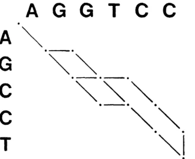
Affine path graphs. If linear gap costs are employed, all optimal alignments of two sequences can simultaneously be represented in a standard
of sequences AGCCT and AGGTCC are represented by the five overlapping paths of the linear path graph in Figure 3-1. For affine gap costs, however, a linear path graph can be ambiguous in indicating precisely which paths are optimal. For example, if w(x)
=
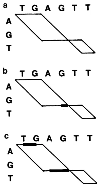
1 + x, sequences AGT and TGAGTT have a minimum alignment cost of 5. Panels a-c of Figure 3-2 show all threeoptimal alignments with this cost and the corresponding simple path graphs. In Figure 3-3a these three optimal paths are combined to give a composite graph. This graph contains a fourth path (Figure 3-2d) but fails to indicate that this fourth path is not optimal.
One way to solve this problem is to represent horizontal and vertical
edges more precisely by the eight symbols shown in Figure 3-4a. Their meanings are defined by the following four conventions, which are
illustrated in Figure 3-4b. (1) A path using a horizontal edge whose left
half is bold must also use the horizontal edge to its left. (2) A path using a horizontal edge whose right half is bold must also use the
horizontal edge to its right. (3) A path using a vertical edge whose top half is bold must also use the vertical edge above. (4) A path using a
vertical edge whose bottom half is bold must also use the vertical edge below.
A path graph that employs these symbols and conventions is called an affine path graph. For example, the three optimal alignments in panels a-c of Figure 3-2 are indicated unambiguously by the affine path graph shown in Figure 3-3b. The SS-2 algorithm presented below actually produces the equivalent affine path graph shown in Figure 3-3c.
Figure 3-1. Paths representing the five optimal alignments of AGCCT and AGGTCC.
A G G
TC
C
A
G
c
c
T
Figure 3-2. Four alignments of AGT and TGAGTT, and their path graphs. (a-c) Optimal alignments for w(x)
=
1 + x.(d) A non-optimal alignment.
a T
G A G T T
- -A
G T-COST:
2
+1
+0
+0
+0
+2
5
T G
A
G T T
bT
G A G T T
-
-
A G
-T
COST:
2
1
*0
+0
+2
*0
-5
T G
A
G
T T
T G A G
T T
A
G
T
d
T
G A G T T
A
G
T
AG
~
- -T
COST:
I +0
*2
*1
+ I +0
-5
T G
A
G T T
A G - - T COST: I + 0 + 2 * I+ 0 + 26
T G
A
G
T T
A
G
T
A
G
T
c
Figure 3-3. Composite path graphs representing the optimal alignments of AGT and TGAGTT for w(x)
=
1 + x.(a) The linear path graph.
(b) An affine path graph representing only the optimal alignments.
(c) The affine path graph produced by the SS-2 algorithm.
a
T
G A G TT
A
G
T
b
T
G A G TT
A
G
T
C
T
G A G T T
A
G
T
Figure 3-4. New edge symbols and their meaning.
(a) Eight symbols for horizontal and vertical edges.
(b) No path using the central edge may use the dotted edges.
b
% %4 .4 I .4 I .4 S 'I .4 U .4 .4 I .4 .4 .4 .4 .4 .4 .4 .47
I
.4 .4 .4 .4 4.K::4
I .4When affine gap costs are used, the minimum cost of continuing a path from a given node to the lower right node of the graph may depend upon whether the given node was entered using a vertical, horizontal or diagonal edge. Paths that enter a node through different edges may have different optimal continuations. Thus new edge symbols, such as those in
Figure 3-4a, are necessary if all and only the optimal paths are to be represented in a single path graph. Using affine gap costs w(x)
=
V + Ux is equivalent to charging V + U for the first null in a gap and U for each subsequent null. Since any path that uses a vertical or horizontal edge has already opened a gap, each subsequent null in the gap will have identical cost U. Thus all paths that enter a node through a given edge will have the same optimal continuations. Therefore the edge symbols of Figure 3-4a provide sufficient modification of the linear path graph to indicate precisely all and only the optimal alignments for affine gap costs.When non-affine gap costs are employed, however, even an affine path graph will not suffice in the general case to represent accurately all and only the optimal alignments of two sequences. For example, if w(1) = 1.2 and w(x) = 0.7 + 0.7(x) for x > 1, there are two optimal alignments of the sequences AGTCGA and GTTACCG (Figure 3-5a). A linear path graph containing the paths that represent each of these alignments appears in Figure 3-5c. It is not possible to use the horizontal edge symbols of Figure 3-4a in this graph in a way that includes both optimal alignments but excludes the two non-optimal alignments shown in Figure 3-5b. Further generalization of the vertical and horizontal edge symbols, however, would allow precise
Figure 3-5. Non-affine gap costs.
(a) The two optimal alignments of AGTCGA and GTTACCG for w(1)
=
1.2 and w(x)=
0.7 + 0.7(x) when x > 1.(b) Two non-optimal alignments.
(c) A composite path graph representing the optimal alignments.
A
G
T
C
G
A
COST: I + *0
+1.2
+0
*1
+1
-
5.2
G
T
T
A
C
C
G
A G T - - -COST:1.2
+0
+0
+1.2
+0.9
+0.7
+C
G
A
0
+0
+1.2
- G T T A C C Gb
A
G
T
COST: I 1 +0
+1.2
+0.9
+C
G
A
0
+0
+1.2 -5.3
G
T
T
A
C
C
G
A
G
T
-C
G
A
COST:1.2
+0
+0
+1.2
+0.9
+0
+1 1
G
T
T
A
C
C
G
C
G T T A
A
G
T
C
G
a
N
5.2
a 5.3C C G
representation of the optimal alignments implied by these gap costs. For general gap costs, a set of pointers can be used at each node to indicate from which nodes above or to the left optimal alignments can come.
An alignment algorithm for affine gap costs. An extension of Gotoh's
algorithm is presented here that finds all and only the optimal alignments of two sequences for affine gap costs and represents them by an affine path graph in the manner described above. Let the affine gap costs be
w(x) = V + Ux. In place of the arrays P and R two one-dimensional number arrays, and in place of array Q a variable, provide sufficient storage (Gotoh, 1982). The three rectangular arrays are used here for ease of exposition.
The SS-2 algorithm consists of the following 11 steps. It calculates the minimum alignment cost, RM,N, and an affine path graph containing all and only those paths that represent optimal alignments of sequences X and Y. All statements involving a negative index should be omitted.
INITIALIZATION. Execute step {11.
M) Initialize the number and bit arrays:
For j from 0 to N, set P 09 to +w and R
,
to V + Uj.For i from 0 to M, set Qi,0 to +o and Ri,0 to V + Ui. Set R0,0 to 0.
Set bit arrays a-g uniformly to 0. Set cM+1,N+1 to 1.
COST ASSIGNMENT. For i from 0 to M and j from 0 to N, execute steps {2} to {7}.
{2} Find the minimum cost of a path ending at node Nij and using edge
V .
Set Pij to U + min (Pi-i,j, Ri..1, + V).
{3) Determine if cost Pij can be achieved using edge Vi_ ,j and if it can be achieved without using edge V
If Piqj = P + U, set di.ij to 1.
If P
=
Ri-ij + V + U, set ei.ij to 1.{4} Find the minimum cost of a path ending at node Nij and using edge
Hi~j:
Set Q to U + min (Qi,j_-, Rigj.. + V).
(5} Determine if cost Qi, can be achieved using edge Hijjl and if it can be achieved without using edge H
If Qi
=
Qi,9_, + U, set f to 1.If Qi
=
Ri, j-_ + V + U, set gv j-, to 1.{6) Find the minimum cost of a path ending at node N j:
Set R to min (PJ, Q ij Ri + c(xivyj)).
(7}
Determine if cost Rij can be achieved by using edge Vi,jg Higj or Dii:If Rig = Pig , set ai, to 1. If R = Qij' set bij to 1.
EDGE ASSIGNMENT. For i from M to 0 and j from N to 0, execute steps {81 to {11}.
{81 If there is no optimal path passing through node N which has cost R at node Ni,j9 remove edges V, Hi and D :
If (ai+, j = 0 o ,j
=
0) and (bi,j+1 = 0 or gj =0) and (c i+1,j+1 = 0),set ai, bij and cij to 0.
{9} If no optimal path passes through Ni, proceed to the next node: If a,+1 , j = bi, j+1 = ci+1 , j+1 = 0 9
skip steps {10} and {111.
(10} If edge Vi+,,j is in an optimal path and requires edge Vi,j to be in an optimal path, determine if an optimal path that uses edge Vj+1,j must use edge V and the converse:
If a,+,j = 1 and d = 1,
[set di+1,j to 1 - ejj set ejj to 1 - ai,j and] set aij to 1.
[Otherwise, set di+,
j
and e to 0.]{11} If edge H j+1 is in an optimal path and requires edge Hi j to be in an optimal path, determine if an optimal path that uses edge Hi, j+1 must use edge Hij and the converse:
If b ij+ 1 = 1 and f = 1,
[set f ij+1 to 1 - g , set gi,j to 1 - bi,j and] set bij to 1.
Comments on the SS-2 algorithm. The meaning of the bit arrays changes during the execution of the algorithm. Let an (i,A) path be a path from
N0,0 to N . After the cost assignment section is complete, the seven bit arrays store the following information:
ai = 1 iff an optimal (i,j) path uses Vjj. bi
=
1 iff an optimal (i,j) path uses Hi.C
=
1 iff an optimal (i,j) path uses Dij.di
=
1 iff among (i+i,j) paths through Ni1 , an optimal one uses V il.ei
=
1 iff among (i+1,j) paths through Ni, an optimal one does not use V ,= 1 iff among (i,j+i) paths through Ni, an optimal one uses Hi, f
gi = 1 iff among (i,j+i) paths through Ni, an optimal one does not use H i.
After the edge assignment section is complete, the seven bit arrays store the affine path graph, as illustrated in Figure 3-6 and described below:
ai,j 1 = 1 iff an optimal (M,N) path uses V . bii = 1 iff an optimal (M,N) path uses Hi. ci, = 1 iff an optimal (M,N) path uses Dii.
dii = 1 iff every optimal (M,N) path that uses Vij also uses Vi-1 ,j. (The top half of Vi, is bold.)
ei1 = 1 iff every optimal (M,N) path that uses Vij also uses Vi+1, j (The bottom half of V is bold.)
Figure 3-6. Bit array assignments. Arrays a-c correspond to full edges and d-g to half edges.
a
b
f
I
d
e
9
Hi,j-i. (The left half of Hjj is bold.)
gi,j
=
1 iff every optimal (M,N) path that uses Hjj also uses Hi,j+1' (The right half of Hi is bold.)Note that if aij = 0, bits d and e are meaningless. Similarly, if bitj = 0 fij and gj are meaningless. Table 3-1 shows the values of the number and bit arrays after the cost and edge assignment for sequences
X = AGT and Y = TGAGTT where w(x) = 1 + x. The affine path graph for this example is presented in Figure 3-3c.
Since the algorithm involves a fixed number of steps for each node, its execution requires O(MN) steps. In the initialization step, O need only be a number larger than any number with which it will be compared during execution of the algorithm; the number 2V + U max(M,N) + 1 will suffice. The bit cM+1,N+1 is initially set to 1 so that the conditions of steps (81 and (9) are false for node NM,N If the four expressions in brackets in steps {10} and {11} are omitted, the linear path graph
represented by bit arrays a-c contains all and only those edges that are
part of some optimal path; such a graph often contains non-optimal paths.
All seven bit arrays are still required to find these edges. While a specific set of substitution costs has been used in all examples in this paper, the SS-2 algorithm allows any set of substitution costs to be
employed. Also, slight modification will allow it to employ different sets of affine gap costs for terminal and interior gaps. When the SS-2
algorithm is implemented on a computer lacking bit storage, the seven bits associated with a given node may conveniently be packed into a single byte.
Table 3-1. Number and bit arrays during execution of the SS-2 algorithm
Node After Cost After Edge
Index Assignment Assignment
i j P Q R a b c d e f g a b c d e f g 00 0 1 0 2 0
3
0
4
0 506
10 1 11
2 13 114 15 16 20 2 1 2 2 2 3 2 4 2 5 2 630
3 1 3 23 3
3 4
3 5
3 6
co 2 03
CO 4 co5oo 6
co7
2co 4 4 5 36 4
7 58 6
9 7
3-
c
3 5
5 5
5 3 7 48 5
9 6
4 co 4 63 5
5 5
5 4
7 5
8 5
01 1 0 1 0 1 0 10 1 000
01 0 1 1 0 1 1 1 0 100 0
01 0 1 0 1 10 11 1 00 0
01 0 1 01 0 1 1 0 0 10 0
0
*1 0 1 0 1 0* 01* 0 * * 0*1* 0.1 011 0*1 0.1 01* 0 0 0 0 0* 01* 01* 011 01* 0110*1* 0*1* 1**1Starred bits are meaningless. Bits with index i = 4 or j = 7 do not change after initialization, and are not shown.
Previous algorithms. If w(x)
=
5 + x, a single optimal alignment exists for sequences AAAGGG and TTAAAAGGGGTT (Figure 3-7). This alignment can not be found by Gotoh's algorithm. It saves only the edge bit arrays a-c during cost assignment in the f orward direction. Steps corresponding to steps {31 and {5} of the SS-2 algorithm are absent. Gotoh's algorithm then repeats the cost assignment in the reverse direction, which saves additional edges, and finds a path with as few turns as possible that uses only saved edges. Since the two edges marked by arrows in the graph of Figure 3-7 are not saved during either the forward or reverse costassignment, neither edge can appear in the path found by Gotoh's algorithm. Thus the path shown in Figure 3-7 is not found by Gotoh's algorithm even though it represents the only optimal alignment.
If w(x)
=
1 + x, sequences AGT and TGAGTT have only the three optimal alignments shown in panels a-c of Figure 3-2. Taylor's algorithm for finding all optimal alignments (Taylor, 1984) saves at each node one vertical and one horizontal pointer for path traceback. Such a pointer system can find any pair of optimal alignments or all four alignments of Figure 3-2, but it can not find precisely the three optimal alignments. In order to identify all and only the optimal alignments in the general case, a pointer system similar to that described by Smith et al. (1981) or Taylor (1984) must allow for an arbitrary number of pointers at each node, wheremany bits may be required to represent each pointer. In contrast, the system described above requires the storage of only seven bits per node even when gaps of arbitrary length are present. The optimal alignments can easily be represented by the corresponding affine path graph.
Figure 3-7. The optimal alignment of AAAGGG and TTAAAAGGGGTT for
w(x)
=
5 + x. Arrows indicate two edges of the path graph not saved by Gotoh's algorithm.T T A A A
AGGGGT
T
A
A
A
G
+ +
G
G
A A A - - - G G GCOST:
I *1
0
6 +I II
+0
+1 +1
-15
T T A A A A G G G G T TAlternatively, all optimal alignments may be extracted from the bit arrays a-g and output linearly, as shown on the right of Figure 3-2. When
non-affine gap costs are employed, a generalization of this system may be
inferior to a system of pointers.
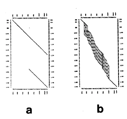
A biological example. The advantage of using affine gap costs when comparing biological sequences is illustrated by two DNA sequences for interleukin 2 (IL-2), an important regulator of T-cell clonal expansion. The DNA sequences code for human IL-2 (Taniguchi et al., 1983) and murine IL-2 (Yokata et al., 1985). The DD algorithm (see Chapter V) was used to search for interesting gap-free subalignments of the two IL-2 sequences using similiarity function si (see Chapter IV). Two of the four best subalignments found were human segment 65-107 with mouse segment 77-119 (43 nucleotides) and human segment 91-299 with mouse segment 133-341 (209 nucleotides). The ends of these subalignments overlap, as shown by the two paths in Figure 3-8a for that part of the DD graph involving human segment 76-107 (H) and murine segment 88-149 (M). Joining these two
subalignments requires a net deletion of 30 nucleotides from M, which can be achieved by inserting one or more gaps into segment H.
Using the SS algorithm (Sellers, 1974a,b) and gap costs w(x) = 2x (Erickson and Sellers, 1983) to align segments H and M produces a large number of optimal subalignments (Figure 3-8b). Because it costs nothing to open a gap, every optimal alignment contains at least 12 separate gaps in segment H, as illustrated by line H1 of Figure 3-9. These alignments imply that at least 12 insertions or deletions are needed to explain the
Figure 3-8. Five path graphs for two DNA sequences from interleukin 2. Vertical sequence M is a 62-nucleotide murine segment and horizontal sequence H is a 32-nucleotide human segment.
(a) Part of a larger DD path graph.
(b) The linear path graph for w(x)
=
2x; paths contain 12-18 gaps.(o) The affine path graph for w(x)
=
0.5 + Ux and U k 1; paths con 3-11 gaps.(d) The affine path graph for w(x) = 1 + Ux and U 1 1; paths conta 1-3 gaps.
(e) The affine path graph for w(x) = V + Ux, V > 1 and U k 0.5; pa
contain only 1 gap.
?CTO C.40S,0Mac a tCTS 900C To . 0 00 a, 120 128 ?FtoCjk**SPA^OA Cos C1 A :40clsh CA ;
a
I I
a
LS 14. 4 lo I I I I I I II it "CS 6"eoat& C~A * t CTONCAI"jo &o110 1 its L&S1
I~
40144
j
46 II I
I I
I I I
b
tainin
thsFigure 3-8. (Continued). Five path graphs for two DNA sequences from
interleukin 2. Vertical sequence M is a 62-nucleotide surine segment and
horizontal sequence H is a 32-nucleotide human segment. (a) Part of a larger DD path graph.
(b) The linear path graph for w(x) = 2x; paths oontain 12-18 gaps.
(c) The affine path graph for w(x) = 0.5 + Ux and U 1 1; paths conta
3-11 gaps.
(d) The affine path graph for w(x) = 1 + Ux and U 1 1; paths contain
1-3 gaps.
(e) The affine path graph for w(x) = V + Ux, V > 1 and U k 0.5; path contain only 1 gap.
1 1 1 1
?
1 II
TVFCfA a r C CT* tMCO*sOCAC
I I I t I I 1I ?CreCAAAOMlatAtc eC041CTOSOCiA 0 Is 29 &as 143 3. !li
. 103 jog 34 ?~t5CSAAS~AOSCOC5OCTh2SSCTSS5OCA 1 1 1 3 11 ii
*s 3 -.I::
SS14 s t aI ISO' i i 14 349d
I I
I
I
I I
11
?t .5 etAAMACA C4ca0t C ISTOO" to,
rT0C ot 0At Or A : Aas cra 'ah C saT 0$ ,A
I
e
I I
I
e
in
3
12. 14, .44 INFigure 3-9. Three representative optimal alignments of murine segment M and human segment H from interleukin 2. Each of the lines H1-H3 is aligned with line M. Smaller letters are different from the corresponding letters in M.
88
100
110
120
130
140
149
M
TCTACAGCGGAAGCACAGCAGCAGCAGCAGCAGCAGCAGCAGCAGCAGCAGCACCTGGAGCA
Hi TCTACA----AAG-A-A--A--A-CA-CA-CAGCT--A-CA--A--A-C---TGGAGCA
H2 TCTACAAAGAAAACA---CAGCTACAACTGGAGCA
H3 TCTACAAAGAAAACACAGCTACAAC---TGGAGCA
76 80
90
100
101
107
segment. Such a large number of events is considered to be unlikely.
The number of insertions or deletions needed becomes smaller when a positive cost V is imposed for opening a gap (Figure 3-8c,d,e). For V > 1 and U 0.5, all 30 nulls must be joined into a single gap, which can be inserted into any one of 11 different places in segment H (Figure 3-8e). Specifically, it can be placed after nucleotide 90 (line H2 of Figure 3-9), after nucleotide 100 (line H3 of Figure 3-9), or after any nucleotide in between. Since murine segment 103-132 encodes 10 glutamine residues, the alignment of lines M and H2 in Figure 3-9 seems the most plausible. Our
experience in comparing nucleotide sequences using affine gap costs suggests that the costs w(x) = 2.5 + 0.5(x) are useful.
Concave gap costs. The algorithm of Waterman et al. (1976) allows arbitrary gap costs w(x). It finds the optimal alignment cost by setting Ritj = min [(Ri-k,j + w(k))k<i, (Rij.l + w(l)),<jg Ri_,j_ + c(xjyj)]
The time complexity of this algorithm is O(MN2
).
Waterman (1984b) has recently described two new algorithms for concave gap costs that he conjectures have time complexity essentially 0(MN). It is shown below that the first of these algorithms has worst-case time complexity at least 0(M2N). For reasonable concave gap costs its average time complexity is also O(M2
N). This algorithm therefore is asymptotically better than that of Waterman et al. (1976) for sequences with greatly
different lengths, but for the usual case of sequences with approximately equal length it is better by at most a constant factor. The average time complexity of the second algorithm of Waterman (1984b) is difficult to
analyze. Its worst-case time complexity appears to be 0[max(M3,MN)].
DEFINITION. Gap costs w(x) are concave (Waterman, 1984b) if for all ij,k > 0, w(i+j+k) - w(i+k) w(j+k) - w(k).
Waterman's first algorithm (1984b) for finding the minimum cost, RMN of aligning sequences X and Y using concave gap costs can be written thus:
Mi} For i from 0 to M, set Ri,0 to w(i) and the set Si to the empty set. For j from 1 to N, set R
j
to w(j) and the set T to the empty set.{2} For i from 1 to M and j from 1 to N:
Set P to min [Ri 1 + w(1), (Rkj + w(i-k))keT.J. If P = Ri.ij+ w(1), add i-1 to the set T .
Set Q to min [Riv.. 1 + w(1), (Rik + w(j-k))kcSi1' If Q
=
R u 1 + w(1), add j-1 to the set Si. Set Ruj to min [P, Q, Riljl + c(xi,yj)].Waterman conjectures that
ISil
grows no faster than log(j) and 'T1 nofaster than log(i). He concludes that the time complexity of the algorithm is effectively O(MN). An example is presented below in which 'Sit grows
linearly with j for j < i and 1T I grows linearly with i for i < j. This alone renders the time complexity of the algorithm O(M2
N); any assumption may be made about the behavior of ISiI as j->o.
Let c(x,y) = 0 if x = y and 1 otherwise, and assume that
w(i+1) > w(i) > 0 for all i
>
0. Let X = Y = AAA... AA. During iteration (i,j) of step {2}, P = R + w(1) if and only if i < j+1. Similarly,Q = R, + w(1) if and only if j < i+1. After completion of iteration (ij), IT I
=
min(ij+1) andISI1
=
min(i+1,j). The minimization during iteration (i,j) thus requires examining more than 2 min(i,j) values. Therefore the algorithm has worst-case time complexity at least O(M2N).Gap costs for which the marginal cost of a null is less than half the mean cost of aligning two elements do not seem appropriate. With such gap costs, the optimal alignment of two long sequences frequently consists of
one long deletion and one long insertion. This observation motivates the following definition.
DEFINITION. Gap costs w(x) are reasonable if limx>. [w(x+1)-w(x)) > 6/2 where F is the expected value of c(x,y) for letters x and y chosen randomly with an appropriate distribution.
When two arbitrary sequences are aligned using reasonable concave gap costs it is usually the case that Q
=
Ri, _, + w(1) whenJ
< i+1: on the average two nulls are replaced by a pair of aligned elements. Thus for reasonable gap costs the algorithm's average as well as its worst-case time complexity is at least O(M2N).Waterman (1984b) suggests that his first algorithm can be improved as follows. Whenever Q
=
Rij. 1 + w(1) in step {2}, for each kESi solveRij. 1 + w(1+h) = Rik + w(j-k+h) [3.1)
for h. If there is no solution or if
J+h
> N then remove k from S i. Ifj+h
< N then Ri,k need not be considered when calculating Ri,x untilcalculations are done for T ,
The worst-case time complexity of this algorithm depends strongly upon the function w(x) and is difficult to analyze. Yet consider sequence X consisting of M C's and sequence Y consisting of M A's followed by an arbitrary number of C's. For reasonable concave gap costs ISjj = 1 while j M+1. For j > M+1, however, it appears that |SA) can grow linearly with j-M at least until j reaches M+1+i. If N 2M this requires a total of O(M3) solutions of equation 3.1. The worst-case time complexity of the algorithm therefore appears to be 0[max(M3,MN)J for at least some concave gap costs.
For average sequences and reasonable gap costs, while j 5 i it is expected not only that Q
=
Ru,1-i + w(1) but also that equation 3.1 has no solution. Therefore ISij should stay near 1 for j i. It is not clear how ISgj grows on the average forj
> i. The average time compl'exity of Waterman's second algorithm (1984b) thus remains an open question.Conclusion. In this chapter it has been shown how to find in O(MN) time all and only the optimal alignments of two sequences using affine gap costs. Previously, Waterman et al. (1976) had shown how to find the
optimal alignments in O(MN2) time, Gotoh (1982) how to find the optimal alignment cost in 0(MN) time, and Taylor (1984) how to find at least one of the optimal alignments in O(MN) time.
Further, it has been shown that Waterman's algorithms (1984b) for concave gap costs have worst-case time complexity at least O(M3). It remains a challenge to find an O(MN) time algorithm for concave gap costs.