Publisher’s version / Version de l'éditeur:
Nano Letters, 14, 12, pp. 7107-7114, 2014-11-14
READ THESE TERMS AND CONDITIONS CAREFULLY BEFORE USING THIS WEBSITE.
https://nrc-publications.canada.ca/eng/copyright
Vous avez des questions? Nous pouvons vous aider. Pour communiquer directement avec un auteur, consultez la première page de la revue dans laquelle son article a été publié afin de trouver ses coordonnées. Si vous n’arrivez pas à les repérer, communiquez avec nous à [email protected].
Questions? Contact the NRC Publications Archive team at
[email protected]. If you wish to email the authors directly, please see the first page of the publication for their contact information.
NRC Publications Archive
Archives des publications du CNRC
This publication could be one of several versions: author’s original, accepted manuscript or the publisher’s version. / La version de cette publication peut être l’une des suivantes : la version prépublication de l’auteur, la version acceptée du manuscrit ou la version de l’éditeur.
For the publisher’s version, please access the DOI link below./ Pour consulter la version de l’éditeur, utilisez le lien DOI ci-dessous.
https://doi.org/10.1021/nl503581d
Access and use of this website and the material on it are subject to the Terms and Conditions set forth at
Polarization entangled photons from quantum dots embedded in
nanowires
Huber, Tobias; Predojević, Ana; Khoshnegar, Milad; Dalacu, Dan; Poole,
Philip J.; Majedi, Hamed; Weihs, Gregor
https://publications-cnrc.canada.ca/fra/droits
L’accès à ce site Web et l’utilisation de son contenu sont assujettis aux conditions présentées dans le site LISEZ CES CONDITIONS ATTENTIVEMENT AVANT D’UTILISER CE SITE WEB.
NRC Publications Record / Notice d'Archives des publications de CNRC:
https://nrc-publications.canada.ca/eng/view/object/?id=58c9a609-e3bb-4e35-adad-38b91b86d82d https://publications-cnrc.canada.ca/fra/voir/objet/?id=58c9a609-e3bb-4e35-adad-38b91b86d82dPolarization Entangled Photons from Quantum Dots Embedded in
Nanowires
Tobias Huber,*
,†Ana Predojević,
†Milad Khoshnegar,*
,‡,§Dan Dalacu,
∥Philip J. Poole,
∥Hamed Majedi,
‡,§and Gregor Weihs
†,‡†
Institut für Experimentalphysik, Universität Innsbruck, Technikerstr. 25, 6020 Innsbruck, Austria
‡
Institute for Quantum Computing and§
Waterloo Institute for Nanotechnology, University of Waterloo, 200 University Ave. West, Waterloo, Ontario N2L 3G1, Canada
∥National Research Council of Canada, 1200 Montreal Road, Ottawa, Ontario K1A 0R6, Canada
ABSTRACT: In this Letter, we present entanglement generated from a novel structure: a single InAsP quantum dot embedded in an InP nanowire. These structures can grow in a site-controlled way and exhibit high collection efficiency; we detect 0.5 million biexciton counts per second coupled into a single mode fiber with a standard commercial avalanche photo diode. If we correct for the known setup losses and detector efficiency, we get an extraction efficiency of 15(3) %. For the measured polarization entanglement, we observe a
fidelity of 0.76(2) to a reference maximally entangled state as well as a concurrence of 0.57(6).
KEYWORDS: Quantum optics, polarization entanglement, quantum dots, nanowires
L
inear optical quantum computation1 as well as mostquantum communication protocols2 require photon entanglement. Additionally, entanglement interconnects the nodes of a quantum network3 and enables different processor architectures and an increase of computational power.4 Quantum dots are promising candidates for generating polarization entangled photon pairs from the biexciton−exciton recombination cascade.5,6 In contrast to other sources of entangled photon pairs,7in quantum dots it is possible to create photon pairs deterministically in a coherent way,8 and they possess inherent subpoissonian photon statistics.9 Nanowire (NW) quantum dots were proposed to deliver superior performance as entangled photon pair sources because of their high symmetry10 and considerably enhanced light extraction efficiencies of axial excitation and collection.11−13 Although a lot of experimental efforts focused on the generation of entangled photon pairs from semiconductor quantum dots,14−19 we are the first to report on the
experimental realization of entangled photon pairs from NW quantum dots. Furthermore, NW quantum dots are advanta-geous in terms of fabrication simplicity; fewer steps are involved in growing and isolating single emitters. They can be positioned homogeneously at predefined positions (see Figure 4c),20−22 and the versatility in the axial and radial growth of III−V nanowires23 allows to manipulate both their electronic and optical properties. The excitonic energy states of NW quantum dots can be deterministically modified by controlling the growth parameters. Finally, single quantum dots can be easily stacked up in a nanowire,24 forming quantum dot molecules with unprecedented design flexibility.
Sample Structure. The NW quantum dots investigated here are ternary In(As)P insertions embedded inside [111]-oriented tapered InP nanowires grown in the wurtzite phase surrounded by a cladding (see Figure 1a). The radial growth of clad InP nanowires provides the option to increase their thickness for optical confinement and allows for coupling between the quantum dot dipole and the nanowire guided modes. From the dispersion diagram of the guided modes in a cylindrical waveguide, we can infer that, beyond the fundamental mode, the second mode that the quantum dot can couple to emerges for DD> 0.23λ0.25Here, DDstands for
the nanowire diameter, and λ0is the mode wavelength in free
space. To achieve the highest extraction efficiency the optimal range of cladding diameters has been numerically demonstrated to be 0.2 < DD/λ0< 0.25.12,26 This means that the extraction
efficiency is not just a function of the number of supported modes. Rather it relies on how well the optical power in the guided modes can couple into the low-index medium (here vacuum). The s-shell excitonic resonances of the quantum dots under study were tuned to be around 910−920 nm (see Figure 1b); hence the cladding diameter is set to ∼200 nm (DD< 0.23
×910 nm) to avoid multimode coupling.
The axial aspect ratio ahof NW quantum dots, defined as the ratio between their height hD and diameter, determines the
strength of the single particle localization and tailors the dispersion of the hole. In order to save the oscillator strength
Received: September 17, 2014
Revised: November 10, 2014
Published: November 14, 2014
pubs.acs.org/NanoLett
against the internal [111]-oriented (vertical) piezoelectric field27 which separates the electron and hole wave functions along the nanowire axis and the exchange-induced spin-flip and cross-dephasing processes,28 adequately strong axial quantiza-tion is favorable (ah < 0.3).29 In addition, the single particle
orbitals are very small in very flat quantum dots (ah < 0.15), and they may present larger anisotropic exchange splitting under morphological asymmetries. A moderate axial local-ization (0.15 < ah < 0.3) maintains the hole ground state h0
predominantly heavy hole (hh)-like,30i.e., |Jh
0, Jzh0⟩= |3/2, ±3/
2⟩ (Jh
0 represents the total angular momentum of the s-shell
hole); thus the quantum dot dipole effectively couples only to circularly polarized light. That the NW quantum dot emission is mostly circularly polarized if collected along the NW axis was also found in ref 31. The final height of the clad nanowire, i.e., LNWin Figure 1a, reaches approximately twice the height of its
core. Details on the growth process can be found elsewhere.23 Methods. The sample was held at 5 K in a temperature-stabilized liquid flow cryostat. The quantum dots were pumped nonresonantly (λexc= 835 nm using a Ti:sapphire laser in cw or
ps-pulsed mode), above the donor−acceptor recombination level usually observed at ∼1.44 eV and in proximity to the wurtzite InP band gap ∼1.50 meV, to photogenerate carriers in
the nanowire continuum. The excitation beam was focused on the spatially isolated nanowire from the side. The quantum dot photoluminescence was collected by an objective lens with a numerical aperture (NA) of 0.7 and dispersed by grating spectrometers (spectral resolution ∼0.02 nm) in order to separate the exciton X0 and biexciton XX0photons and send
them to different polarization analyzers and photon detectors. We applied avalanche photodiodes (APD) with ∼300 ps temporal resolution for correlation experiments not requiring a high time resolution and fiber-pigtailed single-photon detection modules from Micro Photon Devices (MPD) with a high temporal resolution of 35 ps for polarization entanglement measurements. The high-resolution detectors had a quantum efficiency below 5% at wavelengths above 900 nm which leads to integration times of 20 min per projection to resolve the cross-correlation pattern. A time-tagging module was utilized to record correlations between the detection modules. The typical count rate of the MPD detectors during the correlation measurements was ∼65 kHz for X0and ∼23 kHz for XX0after
polarization projection.
We performed fine-structure splitting (FSS) and correlation measurements on the emission of the NW quantum dots using the experimental setup shown in Figure 1d.
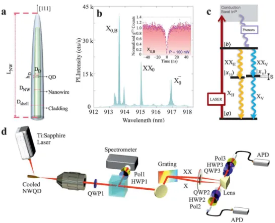
Figure 1.Schematic, spectrum, and energy scheme of the NW quantum dot and experimental setup. (a) Schematic of a clad NW quantum dot tapered at the top. hD: quantum dot height ∼6−8 nm; DD: quantum dot diameter 28 nm; DNW: nanowire (core) diameter ∼28 nm; Dshell: cladding
diameter ∼200 nm; LNW: nanowire length. (b) Photoluminescence intensity of s-shell excitonic resonances of the quantum dot studied in this paper
(dot A): exciton X0,B, biexciton XX0, and negative trion X0−in continuous-wave (cw) nonresonant excitation with a power of Pexc= 500 nW. The inset
illustrates the normalized autocorrelation counts g(2) from the X
0,B line at low excitation power Pexc= 100 nW, confirming a low multiphoton
contribution. Similar g(2)-patterns are observed for the other spectral features. (c) Energy level structure of the NW quantum dot. The excitation laser
creates charge carriers in proximity to the InP band gap. Electrons and holes can relax into the quantum dot by phonon interactions and can fill the biexciton state |b⟩. The recombination can happen on the left or the right path via the exciton state |xH(V)⟩which is the symmetric (antisymmetric)
superposition of the spin up and spin down |x+(−)1⟩state. (d) Experimental setup. The quantum dot was nonresonantly excited using a ps-pulsed
Ti:sapphire laser. The emission was collected using a high NA objective and was analyzed using either a spectrometer and a CCD-camera or using a fiber-coupled dual output grating spectrometer and APDs. Quarter wave plate (QWP) 1 converts the predominant circular polarization of the emitted photons into the rectilinear basis. Half wave plate (HWP) 1 and polarizer (Pol) 1 were used to measure the fine-structure splitting. QWP 2(3), HWP2(3), and Pol 2(3) were used to project the photon states on distinct polarizations to reconstruct the density matrix of the photon pair.
Nano Letters Letter
dx.doi.org/10.1021/nl503581d | Nano Lett. 2014, 14, 7107−7114
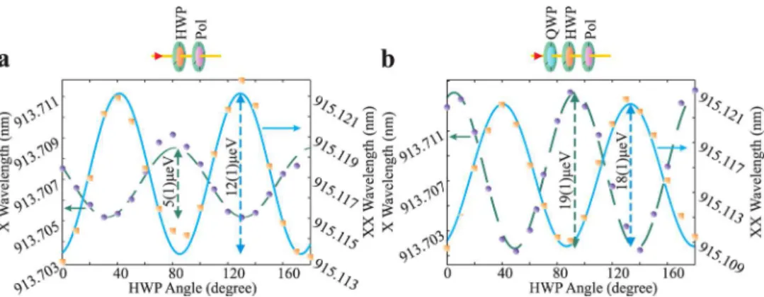
We initially measured the FSS by rotating a HWP in front of a fixed linear polarizer and guiding the quantum dot emission to a grating spectrometer (see Figure 1d). For this measure-ment the quarter-wave plate 1 (QWP1) was removed. The X0
and XX0spectral lines were then fitted to Lorentzian line shapes
to resolve the oscillation of the projected states as a result of the half-wave plate (HWP) rotation. The oscillations showed relatively moderate FSSs in the range of 4(1) to 12(2) μeV for
Figure 2. Fine-structure splitting of dot A. The purple circles (orange squares) and the green dashed (blue solid) fit line represent X0 (XX0)
recombination photons. (a) shows the evolution of resonances when the emission is guided through HWP1 and Pol1. The X0oscillation differs more
than a factor of 2 from the result of the XX0oscillation. We note that, since XX0itself exhibits no exchange splitting, its wavelength oscillation must
arise exclusively from the FSS of the X0state, i.e., SX0= SXX0. (b) shows the same measurement as in (a) with the additional fixed QWP1 in front of
the rotating HWP1. In this case, the amplitudes of X0and XX0oscillations are equal within the error. This measurement shows that the FSS in a
system with predominantly circular polarization is strongly underestimated if the basis of emission is not rectilinear. The slightly unequal amplitudes of the oscillations indicate that the emitters’ polarization was not turned perfectly to rectilinear bases but still has some ellipticity.
Figure 3.Comparison of XX0−X0cross-correlation coincidences with detectors unable to resolve the time oscillations described in the text. (a)
Coincidence counts after projecting the photons onto HH (both photons XX0 and X0 projected onto horizontal polarization H) (red) and
coincidence counts in HV projection (green). Inset: coincidence counts in RR projection (blue) and RL projection (purple), where the projection onto RR gives fewer coincidences than the projection onto RL . Comparing the two plots reflects that the quantum dot dipole primarily couples to the nanowires circular basis as the projections onto HH and HV present no significant difference. (b) Coincidence counts in HH projection (red) and HV projection (green) after inserting QWP1 into the common emission path. Coincidences in the H/V basis are strongly suppressed. A high level of background counts appears here on account of cw pumping. (c) Coincidence counts for different QWP1 settings. The exciton was projected to H, and the polarizer in front of the biexciton was turned. Thus, 0° corresponds to a projection onto HH, and 90° corresponds to a projection onto HV.
all studied quantum dots in different samples. The X0and XX0
oscillations versus the HWP angle are plotted in Figure 2a for dot A. This measurement, however, underestimates the actual FSS because the quantum dot photons couple to the wire’s circular polarization as we will show later in the paper. A measurement on a mixture of circularly polarized light presents no significant variation of the count rate when analyzed via a rotating linear polarizer. For this reason we repeated the FSS measurement with QWP1 in the common emission path. The result can be seen in Figure 2b with a value of S = 18(1) μeV for the FSS. This result shows that the widely used method of a rotating half-wave plate in front of a fixed polarizer can produce results which mask the true value of the FSS if the measured system is not linearly polarized. To rule out the possibility that the polarization rotation was introduced by our setup, we tested our setup with a polarized laser beam and a polarimeter. For the six measured polarizations (horizontal, vertical, diagonal, antidiagonal, right, and left) the error introduced by the setup is less than 1%. Because all quantum dots on the sample show a finite FSS (between 4(1) and 18(1) μeV), we decided to measure the polarization entanglement properties on the brightest dot which is the one introduced here.
For generating an entangled photon pair, the quantum dot state is prepared in the biexciton state (see Figure 1c). After the emission of the biexciton photon, the exciton spin state is entangled with the polarization of the biexciton photon. Since the spin-up and the spin-down exciton states are no eigenstates of the system if they are not degenerate,32the exciton state will evolve with time, e.g., for the emission of a right circular (R) polarized biexciton photon the exciton will result in the state33
|Ψ ⟩ = φ ⟩ − φ ⟩ + − − x i x 1 2(e e ) i i QD /2 1 /2 1 (1)
The phase ϕ = Sτ/ℏ, where τ is the time elapsed between the first and second photon emission, is directly transferred on the phase of the exciton photon when the exciton recombines. Thus, the exciton photon wave function is
|Ψ ⟩ = φ | ⟩ − −φ | ⟩ i 1 2(e L e R ) X i /2 i /2 0 (2)
Considering the two-photon state this will lead to an evolution between the |Φ+⟩ = (1/21/2)(|RL⟩ + |LR⟩) and |Φ−⟩ = (1/
21/2)(|RR⟩ + |LL⟩) Bell states. The state could be rewritten in
the H/V (horizontal/vertical) polarization basis as34
|Ψ⟩ = 1 | ⟩ + φ| ⟩ 2( HH e VV )
i
(3)
or in the D/A (diagonal/antidiagonal) polarization basis where we get an oscillation between the |Φ+⟩ = (1/21/2)(|DD⟩ + |
AA⟩) and the |Φ−⟩= (1/21/2)(|DA⟩ + |AD⟩) state similar to the
R/L basis.
This shows that a change of the phase in an entangled state can be directly measured in a time-resolved correlation measurement by observing the correct polarization projection, e.g., projecting both photons onto R polarization (projection onto RR) should show high coincidence probability for times where the two photon state is in |Φ−⟩ and low coincidence probability when the state is in |Φ+⟩. The opposite behavior is
expected for a projection onto DD. If the oscillation is visible in two complementary bases, the third complementary basis (e.g., H/V basis) should show classical correlations as reported in ref 35, which does not show oscillations.
For the sake of comparison to previously reported measure-ments from entangled photon pairs from quantum dots, it would be beneficial if the basis where classical correlations can be observed were H/V. Unfortunately, in our system this is not the case (see Figure 3a). The figure shows almost equal probabilities for HH and HV, respectively. Classical correlations can be partially observed in the R/L basis (see inset in Figure 3a). To get classical correlations in the H/V basis, we locally rotate the polarization state by inserting a quarter wave plate (QWP1) into the common emission path of both XX0and X0
photons (see Figure 1d for the setup and Figure 3b for the obtained result). For achieving maximum visibility in the H/V basis, we performed several coincidence measurements with different QWP1 settings. For each visibility measurement the polarizer in the X0photon path was fixed to H and the polarizer
in the XX0 photon path was rotated (see Figure 3c). Such a
local rotation of the polarization qubit cannot affect the degree of entanglement but can change the fidelity to a particular desired state.
To quantify the degree of entanglement, a tomographic experiment was implemented with 16 cross-correlation measurements of different combinations of polarization projections.36The NW quantum dots were excited by a pulsed laser to minimize any uncorrelated photons caused by re-excitations in a continuous pumping scheme. Owing to the nonzero FSS, the evolving phase of the photon pair state reduces the time-integrated concurrence.34 We therefore postselect the correlated photons within specific time windows and calculate the fidelity with respect to a reference Bell state for each time interval. Accordingly, a temporal resolution sufficient to resolve the correlation pattern of each window is necessary. The period of the photon pair phase ϕ is predicted to be ∼230(12) ps for an FSS of S ∼ 18(1) μeV (see Figure 2b), i.e., every ∼115 ps the phase of photon pair flips, while its power simultaneously fades according to the finite exciton lifetime (∼2 ns). In order to resolve the oscillations we used highly time-resolving detectors after the spectral filtering and the polarization state projection.
Theoretical Investigation of the Fine-Structure Split-ting. An anisotropic FSS results from the exchange energy caused by the Rashba spin−orbit interaction in combination with a low symmetry of electron and hole orbitals. The anisotropic exchange splitting is theoretically predicted to vanish once the net symmetry of the exciton wave function exceeds C2v.10,37The ideal hexagonal (D6h) or cylindrical (D∞h)
symmetry of [111]-oriented zinc blende (or wurtzite) NW quantum dots leads to C3v-symmetric orbitals, which preserve
the degeneracy of the bright excitons X0,B. This elevated
symmetry character directly originates from the C3vsymmetry
of the strain-induced potentials, including the piezoelectric potential. The origin of the FSS in our NW quantum dots could be explained either by (a) an in-plane (perpendicular to the nanowire axis) asymmetry, namely elongation, (b) off-center growth of the nanowire core, or (c) inhomogeneity of the quantum dot material composition, which all may bring down the symmetry of the net confinement and lift the X0,B
degeneracy. In the following, we discuss each of above potential sources of FSS.
Quantum Dot Elongation. According to the atomistic million-atom many-body pseudopotential calculations by Singh et al., a small level of FSS (∼3−8 μeV) appears upon 5−15% lateral elongation of pure InAs disk quantum dots (hD= 3.5 nm
and DD = 25 nm) embedded in [111]-oriented InP
Nano Letters Letter
dx.doi.org/10.1021/nl503581d | Nano Lett. 2014, 14, 7107−7114
nanowires.10For hexagonal quantum dots of comparable size, a similar range of FSS is expected. In our case of ternary In(As)P insertions with a large fraction of phosphorus (InAs0.2P0.8) and
hD= 6−8 nm, an even more pronounced elongation is required
to induce this amount of FSS as the quantum dot confinement and piezoelectric potential are both weak and the orbitals are comparatively dilute. We do not observe any evident sign of lateral elongation in scanning electron microscopy (SEM) images showing the cross sections of the nanowire cores (see Figure 4b). On average, a small elongation ratio (<5%) is confirmed for the investigated nanowires, which is unable to induce a significant level of FSS (>10 μeV).
Off-Center Nanowire Growth. Another source of FSS could be the dislocation of the quantum dot insertion with respect to the nanowire axis due to the displacement of the gold particle during the temperature ramp. Figure 5a shows the plan view SEM image of a clad nanowire, where the nanowire core is misaligned with the axis of the cladding. A considerable displacement, as shown in the inset of Figure 5a, induces a nonuniform strain field and piezoelectric potential. We modeled the impact of a moderate displacement (ΔD = 14
nm <0.2Dshell) on a hexagonal InAs0.2P0.8quantum dot with hD
= 6 nm and DD= 28 nm embedded inside a 80-nm-thick InP
nanowire (see Figure 5b). The details of the modeling can be
found elsewhere.29Figure 5c shows the single particle orbitals of electrons (e0−e2) and holes (h0−h2) of a quantum dot with
the above specifications. As expected, the single particle orbitals present a C3vsymmetry once the quantum dot is located at the
center of nanowire (ΔD= 0). The bottom panel of Figure 5c
shows the single particle states in a quantum dot 14 nm dislocated along the [11̅0] direction. The C2vsymmetry of the
wave function shows p-states (e1−e2and h1−h2), which signifies
the asymmetry of the underlying strain field. This low symmetry character is not quite visible in the ground state (e0 and h0) because (a) the displacement is limited and the
strain field partially relaxes within the cladding, and (b) the compressive strain experienced by the InAs0.2P0.8 insertion
inside an InP matrix is weak. Therefore, we expect that only a small part of the FSS, namely, <5 μeV, can be induced by the quantum dot dislocation in our investigated samples.
Compositional Inhomogeneity. The above discussions suggest that the FSS in our NW quantum dots mostly originates from the compositional anisotropy rather than the geometrical asymmetry. It is well-known that any anisotropy along the main quantization axis can lead to a polarized piezoelectric field and FSS in SK dots.27,38 NW quantum dots are however immune to these types of (geometrical) axial anisotropy;29 thus the FSS observed in our samples must be
Figure 4.Scanning electron microscopy (SEM) images of the nanowires. (a) SEM image of a single tapered nanowire, which is spatially isolated for convenient optical access. (b) Top view SEM image of a clad nanowire showing the in-plane hexagonal symmetry of its core (and the embedded quantum dot), without any sign of significant elongation. (c) SEM picture of an array of nanowires, showing their homogeneous positioning.
Figure 5.Wave function calculations for off-centered quantum dots. (a) Plan view SEM image of a clad nanowire depicting its cross section. The nanowire core is slightly displaced with respect to the center of cladding. Inset: plan view SEM image of a nanowire core showing a significant displacement off the center. (b) Cross section of numerically modeled InAs0.2P0.8/InP NW quantum dots with hexagonal symmetry. Left, the
quantum dot center and the cladding axis are aligned; Right, the quantum dot center is moved 14 nm along [11̅0] direction with respect to the cladding axis. (c) The probability density of electrons (holes) in the s shell, e0(h0), and p shells, e1−e2(h1−h2) of NW quantum dots introduced in b.
Only the quantum dot region is illustrated. Top: orbitals exhibit C3vsymmetry when the nanowire core is located at the center of cladding. Bottom:
primarily induced by an inhomogeneity of their ternary composition. Versteegh et al.39have recently shown that for thicker QDs the FSS vanishes, with the drawback of longer emission wavelength, but it might be possible to develop a thermal annealing process to get rid of the compositional inhomogeneity and thus decrease the FSS to sub-μeV level for any desired target wavelength.
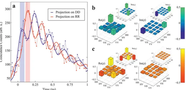
Results. Figure 6a shows the cross-correlation counts for both the RR and DD projections obtained with 35 ps temporal resolution. Here, the oscillatory behavior of photon pair wave function is clearly observable in the corresponding correlation patterns, particularly within the early stages after the cascade initialization. The period of the fitted oscillatory functions τfit=
225(5) ps agrees with the value of 230(12) ps calculated from the FSS value.
In order to identify the photon pair states, the 65-ps-wide shaded areas in Figure 6a were postselected, and the corresponding density matrices ρ were reconstructed using a maximum-likelihood estimation36 from the raw data without any background subtraction. The reconstructed density matrix ρ1for the first time window of 65 ps right after the excitation is
shown in Figure 6b. The inset shows the density matrix ρth1of
the state |Ψth1⟩= (1/(2)1/2)(|HH⟩ + i|VV⟩) to which ρ1has a
fidelity of F = 0.74(2). Since we performed a tomographic measurement, we calculated the fidelity directly from ρ1, F =
Tr(((ρ1)1/2·ρth·(ρ1)1/2)1/2)2, instead of using the correlation
visibility in different polarization bases.40The concurrence of ρ1
is C = 0.57(6). Within the following time window, where the projection of the RR state has a maximum, a phase rotation occurs as could be inferred from the associated density matrix shown in Figure 6c. The fidelity with the reference state |Ψ−⟩=
(1/21/2)(|HH⟩ − |VV⟩) and the photon concurrence were
calculated to be F = 0.69(2) and C = 0.45(2). Increasing the coincidence window of the first analyzed state slowly reduces the fidelity and reaches F = 0.53(3) to the |Ψth1⟩state and F =
0.51(1) to the |Ψ−⟩state when the window is 180 ps. Since the
coincidence window now includes two orthogonal states, a maximally mixed state (with F = 0.5) is expected. To improve the fidelity, a resonant pumping scheme would be beneficial.41 Having a closer look at the fidelities (see Table 1), we find that the state is not only represented in the |ϕ±
⟩subspace. The
highest fidelity we get to a state which is rotated, for both analyzed coincidence windows. We attribute this to a nonperfect state rotation which originates in the coupling of the quantum dot to the nanowire’s circular polarization. The resulting emission might be not perfectly circular but elliptical to some degree. Considering an elliptical photon polarization, the QWP1 will not turn the polarization of the emission to rectilinear basis, introducing an error in the expected photon state.
Conclusion. We utilized temporal selection of quantum correlated photons and observed rather high levels of fidelity, F = 0.76(2) (C = 0.57(6)) and F = 0.70(2) (C = 0.45(2)), despite the comparably fast phase variation of the photon pair state. The periodicity of the phase oscillation was first estimated directly via FSS measurements, then validated by the oscillatory behavior of the cross-correlation patterns. Our results serve as a prototypical assessment of the optical quality of NW quantum
Figure 6.Tomographic measurement of polarization entanglement. (a) shows two specific analyzer settings, while (b,c) shows real and imaginary parts of the density matrices associated with the reconstructed and the corresponding theoretical states. (a) Cross-correlation counts of the DD (red) and RR (blue) projections resolved with 35 ps temporal resolution. Please note that the separation between the obtained data points is only 16 ps. The detectors are still not able to resolve the oscillations fully; otherwise their minima would reach zero. The red and blue curves represent the fits to the correlation functions with oscillations of the same period and amplitude and 180° phase difference, indicating the evolving phase of the photon pair state. The blue curve reaches its local maxima where the red curve has its local minima and vice versa. (b) shows the reconstructed density matrix with photons postselected in a time window of 65 ps immediately after the cascade decay. The insets show the density matrix components of the ideal theoretical state. (c) Similar to (b), but measured at a later time interval of 65 ps (where the projection onto RR (a) has its maximum), once the photon pair phase has evolved.
Table 1. Fidelities of the Reconstructed Density Matrices to Different Maximally Entangled States
reference state F to ρ1 F to ρ2 |ϕ+⟩= (1/√2)(|HH⟩ + |VV⟩) 0.53(2) 0.13(2) (1/√2)(|HH⟩ + i|VV⟩) 0.74(2) 0.50(2) |ϕ−⟩= (1/√2)(|HH⟩ − |VV⟩) 0.29(2) 0.69(2) (1/√2)(|HH⟩ + i|VV⟩) 0.08(1) 0.33(2) (1/√2)(|HH⟩ + ei·70°|VV⟩) 0.76(2) (1/√2)(|HH⟩ + ei·160°|VV⟩) 0.70(2)
Nano Letters Letter
dx.doi.org/10.1021/nl503581d | Nano Lett. 2014, 14, 7107−7114
dots for generating polarization entangled photon pairs. While we were writing this, we found that similar results on entanglement were measured simultaneously by Versteegh et al.39
Reconstructing the Density Matrix. We performed the reconstruction of the density matrix following James et al.,36 and we will give a short summary of the necessary steps here. We do not follow a very strict nor complete theoretical description but rather give the reader a guideline. For more details we would like to refer to the original paper.36The goal of the reconstruction is to find the most likely density matrix ρ̂. What can be measured are coincidence counts n, obtained by performing different projections of the type |ψν⟩, where each ν
stands for a set of given polarizations for exciton and biexciton. The coincidence counts are given by36
ψ ρ ψ
= ⟨ | ̂| ⟩
ν ν ν
n N (4)
where N is a constant which depends on the detectable photon flux. It is convenient to convert the 4 × 4 matrix ρ̂ to a 16-dimensional vector using36
∑
ρ̂ = Γ̂ ν ν ν = r 1 16 (5)The Γ̂ν matrices can be found in Appendix B of James’
paper.36We can now introduce Bμ,ν= ⟨ψν|Γ̂μ|ψν⟩and rewrite eq
4 as nν= N∑μ=116 Bν,μrμ. This can be inverted to give:
36
∑
= ν μ ν μ μ − = − r ( )N 1 (B ) n 1 16 1 , (6)To rewrite ρ̂ as a matrix, we define M̂ν= ∑μ=116 (B−1)ν,μΓ̂μ and
substitute eq 6 into eq 5 and find that ρ̂ = (N)−1∑ν=116 M̂νnν. For
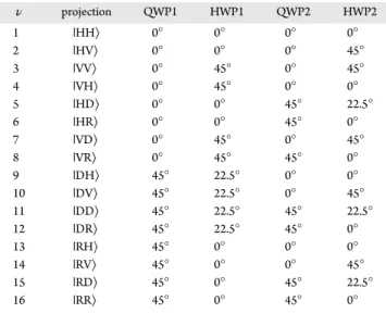
the set of states given in Table 2, the final formula for the density matrix is ρ̂ = ∑ν=116 M̂νnν/∑ν=14 nν.
Unfortunately the obtained matrix is not necessarily physical. This can be fixed, by defining a new matrix ρ̂p = T̂
†
(t)T̂(t)/ Tr{T̂†(t)T̂(t)} where T̂(t) is defined in eq 4.4 7 of ref 36 and
the rules on how to link the entries of ρ̂ with t1,2,...16are defined
in eq 4.6 therein. As we now have a physical guess for our matrix ρ̂p, we can perform a numerical optimization routine to
find the most likely density matrix. This is done by minimizing (numerically) the function:
∑
ψ ρ ψ ψ ρ ψ = ⟨ | ̂ | ⟩ − ⟨ | ̂ | ⟩ ν ν ν ν ν ν = L t t t N n N ( , , ... ) [ ] 2 p p 1 2 16 1 16 2 (7)In our experiment the following values were found for the 16 projections in the first post selected time interval: n1= 151, n2=
19, n3= 34, n4= 100, n5= 85, n6= 86, n7= 84, n8= 72, n9= 77,
n10= 87, n11= 129, n12= 30, n13= 93, n14= 59, n15= 42, n16=
79. The reconstructed density matrix is shown in Figure 6b. For estimating the error on the reconstructed matrix, we performed the above-described reconstruction for 1000 differ-ent sets of random values where the randomness is modeled as Poissonian noise on the measured value.
Additional Cross-Correlation Data.In Figure 7, the time-resolved biexciton exciton cross-correlation for the HH, and the
HV projection is presented to complete the time-resolved data sets for three different bases. The rectilinear and circular data set is shown in Figure 6.
■
AUTHOR INFORMATIONCorresponding Authors
*E-mail: [email protected]. *E-mail: [email protected].
Notes
The authors declare no competing financial interest.
■
ACKNOWLEDGMENTSThe authors thank the funding agencies. This work was funded by NSERC, the European Research Council (project EnSeNa, no. 275531), and the Canadian Institute for Advanced Research through its Quantum Information Processing program. T. H. thanks the Austrian Academy of Sciences for receiving a DOC Fellowship. M. K. thanks the Waterloo Institute for Nano-technology and NSERC’s CryptoWorks21 program for their fellowships. A. P. would like to thank Austrian Science Fund (FWF) for support provided through Elise Richter Fellowship V-375.
■
REFERENCES(1) Knill, E.; Laflamme, R.; Milburn, G. Nature 2001, 409, 46−52. (2) Tittel, W.; Weihs, G. Quantum Infor. Comput. 2001, 1, 3−56. (3) Bennett, C. H. Phys. Today 1995, 8, 24−30.
Table 2. List of Tomographic States and Required Settings for the Waveplates If the Polarizer Is Set to H
ν projection QWP1 HWP1 QWP2 HWP2 1 |HH⟩ 0° 0° 0° 0° 2 |HV⟩ 0° 0° 0° 45° 3 |VV⟩ 0° 45° 0° 45° 4 |VH⟩ 0° 45° 0° 0° 5 |HD⟩ 0° 0° 45° 22.5° 6 |HR⟩ 0° 0° 45° 0° 7 |VD⟩ 0° 45° 0° 45° 8 |VR⟩ 0° 45° 45° 0° 9 |DH⟩ 45° 22.5° 0° 0° 10 |DV⟩ 45° 22.5° 0° 45° 11 |DD⟩ 45° 22.5° 45° 22.5° 12 |DR⟩ 45° 22.5° 45° 0° 13 |RH⟩ 45° 0° 0° 0° 14 |RV⟩ 45° 0° 0° 45° 15 |RD⟩ 45° 0° 45° 22.5° 16 |RR⟩ 45° 0° 45° 0°
Figure 7. Time resolved biexciton−exciton cross correlations in the HH and HV basis. The record resolution is 16 ps, and the detector resolution is 35 ps. No oscillation is visible as expected.
(4) Ward, M.; Dean, M.; Stevenson, R.; Bennett, A.; Ellis, D.; Cooper, K.; Farrer, I.; Nicoll, C.; Ritchie, D.; Shields, A. Nat. Commun. 2014, 5, 3316.
(5) Benson, O.; Santori, C.; Pelton, M.; Yamamoto, Y. Phys. Rev. Lett. 2000, 84, 2513−2516.
(6) Akopian, N.; Lindner, N. H.; Poem, E.; Berlatzky, Y.; Avron, J.; Gershoni, D.; Gerardot, B. D.; Petroff, P. M. Phys. Rev. Lett. 2006, 96, 130501.
(7) Predojević, A.; Grabher, S.; Weihs, G. Opt. Express 2012, 20, 25022−25029.
(8) Jayakumar, H.; Predojević, A.; Huber, T.; Kauten, T.; Solomon, G. S.; Weihs, G. Phys. Rev. Lett. 2013, 110, 135505.
(9) Predojević, A.; Ježek, M.; Huber, T.; Jayakumar, H.; Kauten, T.; Solomon, G. S.; Filip, R.; Weihs, G. Opt. Express 2014, 22, 4789−4798.
(10) Singh, R.; Bester, G. Phys. Rev. Lett. 2009, 103, 063601. (11) Claudon, J.; Bleuse, J.; Malik, N. S.; Bazin, M.; Jaffrennou, P.; Gregersen, N.; Sauvan, C.; Lalanne, P.; Gerard, J.-M. Nat. Photonics 2010, 4, 174−177.
(12) Reimer, M. E.; Bulgarini, G.; Akopian, N.; Hocevar, M.; Bavinck, M. B.; Verheijen, M. A.; Bakkers, E. P.; Kouwenhoven, L. P.; Zwiller, V. Nat. Commun. 2012, 3, 737.
(13) Munsch, M.; Malik, N. S.; Dupuy, E.; Delga, A.; Bleuse, J.; Gérard, J.-M.; Claudon, J.; Gregersen, N.; Mørk, J. Phys. Rev. Lett. 2013, 110, 177402.
(14) Stevenson, R. M.; Young, R. J.; Atkinson, P.; Cooper, K.; Ritchie, D. A.; Shields, A. J. Nature 2006, 439, 179−182.
(15) Dousse, A.; Suffczyński, J.; Beveratos, A.; Krebs, O.; Lematre, A.; Sagnes, I.; Bloch, J.; Voisin, P.; Senellart, P. Nature 2010, 466, 217− 220.
(16) Jayakumar, H.; Predojević, A.; Kauten, T.; Huber, T.; Solomon, G. S.; Weihs, G. Nat. Commun. 2014, 5, 4251.
(17) Juska, G.; Dimastrodonato, V.; Mereni, L. O.; Gocalinska, A.; Pelucchi, E. Nature Photonics 2013, 7, 527−531.
(18) Kuroda, T.; Mano, T.; Ha, N.; Nakajima, H.; Kumano, H.; Urbaszek, B.; Jo, M.; Abbarchi, M.; Sakuma, Y.; Sakoda, K.; Suemune, I.; Marie, X.; Amand, T. Phys. Rev. B 2013, 88, 041306.
(19) Trotta, R.; Zallo, E.; Magerl, E.; Schmidt, O. G.; Rastelli, A. Phys. Rev. B 2013, 88, 155312.
(20) Hertenberger, S.; et al. Appl. Phys. Lett. 2012, 101, 43116. (21) Makhonin, M. N.; Foster, A. P.; Krysa, A. B.; Fry, P. W.; Davies, D. G.; Grange, T.; Walther, T.; Skolnick, M. S.; Wilson, L. R. Nano Lett. 2013, 13, 861−865 PMID: 23398085.
(22) Dalacu, D.; Mnaymneh, K.; Wu, X.; Lapointe, J.; Aers, G. C.; Poole, P. J.; Williams, R. L. Appl. Phys. Lett. 2011, 98, 251101.
(23) Dalacu, D.; Mnaymneh, K.; Lapointe, J.; Wu, X.; Poole, P. J.; Bulgarini, G.; Zwiller, V.; Reimer, M. E. Nano Lett. 2012, 12, 5919− 5923 PMID: 23066839.
(24) Björk, M. T.; Thelander, C.; Hansen, A. E.; Jensen, L. E.; Larsson, M. W.; Wallenberg, L. R.; Samuelson, L. Nano Lett. 2004, 4, 1621−1625.
(25) Bleuse, J.; Claudon, J.; Creasey, M.; Malik, N. S.; Gérard, J.-M.; Maksymov, I.; Hugonin, J.-P.; Lalanne, P. Phys. Rev. Lett. 2011, 106, 103601.
(26) Friedler, I.; Sauvan, C.; Hugonin, J. P.; Lalanne, P.; Claudon, J.; Gérard, J. M. Opt. Express 2009, 17, 2095−2110.
(27) Schliwa, A.; Winkelnkemper, M.; Lochmann, A.; Stock, E.; Bimberg, D. Phys. Rev. B 2009, 80, 161307.
(28) Tsitsishvili, E.; v. Baltz, R.; Kalt, H. Phys. Rev. B 2005, 72, 155333.
(29) Khoshnegar, M.; Majedi, A. H. Phys. Rev. B 2012, 86, 205318. (30) Niquet, Y.-M.; Mojica, D. C. Phys. Rev. B 2008, 77, 115316. (31) van Weert, M. H. M.; Akopian, N.; Kelkensberg, F.; Perinetti, U.; van Kouwen, M. P.; Rivas, J. G.; Borgström, M. T.; Algra, R. E.; Verheijen, M. A.; Bakkers, E. P. A. M.; Kouwenhoven, L. P.; Zwiller, V. Small 2009, 5, 2134−2138.
(32) Bayer, M.; Ortner, G.; Stern, O.; Kuther, A.; Gorbunov, A. A.; Forchel, A.; Hawrylak, P.; Fafard, S.; Hinzer, K.; Reinecke, T. L.; Walck, S. N.; Reithmaier, J. P.; Klopf, F.; Schäfer, F. Phys. Rev. B 2002, 65, 195315.
(33) Wilk, T.; Webster, S. C.; Kuhn, A.; Rempe, G. Science 2007, 317, 488−490.
(34) Stevenson, R. M.; Hudson, A. J.; Bennett, A. J.; Young, R. J.; Nicoll, C. A.; Ritchie, D. A.; Shields, A. J. Phys. Rev. Lett. 2008, 101, 170501.
(35) Santori, C.; Fattal, D.; Pelton, M.; Solomon, G. S.; Yamamoto, Y. Phys. Rev. B 2002, 66, 045308.
(36) James, D. F. V.; Kwiat, P. G.; Munro, W. J.; White, A. G. Phys. Rev. A 2001, 64, 052312.
(37) Altmann, S. L.; Herzig, P. Point-Group Theory Tables; Clarendon Press: Oxford, 1994.
(38) Zieliński, M. Phys. Rev. B 2013, 88, 155319.
(39) Versteegh, M. A. M.; Reimer, M. E.; Jöns, K. D.; Dalacu, D.; Poole, P. J.; Gulinatti, A.; Giudice, A.; Zwiller, V. Nat. Commun. 2014, 5, 5298.
(40) Hudson, A. J.; Stevenson, R. M.; Bennett, A. J.; Young, R. J.; Nicoll, C. A.; Atkinson, P.; Cooper, K.; Ritchie, D. A.; Shields, A. J. Phys. Rev. Lett. 2007, 99, 266802.
(41) Müller, M.; Bounouar, S.; Jons, K. D.; Glassl, M.; Michler, P. Nat. Photonics 2014, 8, 224−228.
Nano Letters Letter
dx.doi.org/10.1021/nl503581d | Nano Lett. 2014, 14, 7107−7114