Audioptimization : global-based acoustic design

Audioptimization: Goal-Based Acoustic Design

Michael Christopher Monks

M.S. Computer Graphics

Cornell University, 1993

B.S. Computer and Information Science University of Massachusetts at Amherst, 1987

Submitted to the Department of Architecture in Partial Fulfillment of the Requirements for the

Degree of

Doctor of Philosophy in the Field of Architecture: Design and Computation at the

Massachusetts Institute of Technology

ROTCi

J

June 1999

L1i

@1999,

The author hereby grants to MIT permission to

reproduce and to distribute publicly paper and electronic copies of this thesis document in whole or in part.

A uthor: . . . .. ... . .. .. . ... . . . . .

Department of Architecture April 30, 1999 C ertified b y : . . . .. . . .. .orsey

U

Associate Professor of Architecture and Computer Science and Engineering Thesis Advisor

A ccepted by: ... ...

Stanford Anderson Professor of History and Architecture Chairman, Department Committee on Graduate Students

R eader: . . . .. . . - . .. . . . ..

Leonard McMillan Assistant Professor of Computer Science

Reader: ...

Carl Rosenberg Lecturer of Architecture

Audioptimization: Goal-Based Acoustic Design

by

Michael Christopher Monks

Submitted to the Department of Architecture on April 30, 1999, in partial fulfillment of the

requirements for the degree of

Doctor of Philosophy in the Field of Architecture: Design and Computation

Abstract

Acoustic design is a difficult problem, because the human perception of sound depends on such things as decibel level, direction of propagation, and attenuation over time, none of which are tangible or visible. The advent of computer simulation and visualization tech-niques for acoustic design and analysis has yielded a variety of approaches for modeling acoustic performance. However, current computer-aided design and simulation tools suffer from two major drawbacks. First, obtaining the desired acoustic effects may require a long, tedious sequence of modeling and/or simulation steps. Second, current techniques for mod-eling the propagation of sound in an environment are prohibitively slow and do not support interactive design.

This thesis presents a new approach to computer-aided acoustic design. It is based on the inverse problem of determining material and geometric settings for an environment from a description of the desired performance. The user interactively indicates a range of accept-able material and geometric modifications for an auditorium or similar space, and specifies acoustic goals in space and time by choosing target values for a set of acoustic measures. Given this set of goals and constraints, the system performs an optimization of surface ma-terial and geometric parameters using a combination of simulated annealing and steepest descent techniques. Visualization tools extract and present the simulated sound field for points sampled in space and time. The user manipulates the visualizations to create an in-tuitive expression of acoustic design goals.

We achieve interactive rates for surface material modifications by preprocessing the ge-ometric component of the simulation, and accelerate gege-ometric modifications to the audito-rium by trading accuracy for speed through a number of interactive controls.

We describe an interactive system that allows flexible input and display of the solution and report results for several performance spaces.

Thesis Supervisor: Julie Dorsey

Acknowledgments

As with any endeavor of this magnitude, many people have contributed to its achievement.

By far the most important influence on this work comes, not surprisingly, from my wife

Marietta. Were it not for her continuous encouragement and support, this effort would have been abandoned well short of its fruition. My son Andrew James has also provided me with the perspective and outlook that enabled me to press on, without being consumed by the

gravity of the project.

Aside from my life support, of the players that filled the most prominent roles in the work itself, my advisor and friend Julie Dorsey assumed the lead. Without her creativity, enthusi-asm, and persuasion my involvement in this project would not have begun. Julie generated the driving force to keep the project vital when it appeared to be headed for difficulties. She never lost sight of what the project could be, while I was focused on what it was.

The project itself is composed ofjoint work done by my research partner Byong Mok Oh and myself. Mok and I shared responsibilities for all aspects of the original work, although like any good team, we each deferred to the other's strengths when disagreements arose. I would like to thank my additional committee members, Carl Rosenberg and Leonard McMil-lan, for their guidance through numerous helpful suggestions and remarks.

My thanks to Alan Edelman and Steven Gortler for sharing their insights in

optimiza-tion, graphics, and overall presentation of early drafts of papers related to this work. I am also indebted to a variety of people from the acoustics community. First, thanks to Leo Be-ranek, for inspirational discussions. I am also grateful to Amar Bose, Ken Jacob and Kurt Wagner for sharing their insights on the project. Thanks goes to Mike Barron, John Walsh

and Mendel Kleiner for their help gathering background information.

Thanks to the UROPs who participated in this project, including John Tsuchiha, Max Chen, and Natalie Garner, for modeling Kresge Auditorium and Jones Halls, writing nu-merous software modules, and experimenting with the system.

Finally, let me acknowledge the lab mates who helped create an enjoyable environment in which to work. Among the most responsible are Mok, Sami Shalabi, Jeff Feldgoise,

Osama Tolba, Kavita Bala, Justin Legakis, Hans Pedersen, Rebecca Xiong, and Jon Lev-ene. Thanks people.

This work was supported by an Alfred P. Sloan Research Fellowship (BR-3659) and by a grant from the National Science Foundation (IRI-9596074). The Oakridge Bible Chapel model was provided by Kurt Wagner of the Bose Corporation.

Contents

2.2.1 Reverberation: Sabine's Formula . . . 25

2.2.2 Statistical Approximations . . . 27

3 Survey of Acoustic Simulation Approaches 29 3.1 Ray Tracing . . . .. . . - - - - . . . . 29

3.2 Statistical Methods . . . .. . . . . 30

3.3 Radiant Exchange Methods . . . . .. . . 31

3.4 Image Source . . . .. . . - - - 32 3.5 Beam Tracing . . . .. . . .. . - -. . 32 3.6 Hybrid Methods . . . .. . - . . . - - . . 33 3.7 Summary . . . .. . .. . . - - - . 33 4 Acoustic Evaluation 35 4.1 Characterization of Sound . . . . 35

4.2 Visualization of Acoustic Measures . . . 38

5 Acoustic Simulation: A Unified Beam Tracing and Statistical Approach 43 5.1 Generalized Beams . . . .. . - . . . 44

5.2 Improved Statistical Tail Approximation . . . 47

5.3 Sound Field Point Sampling . . . . 50

5.4 Multidimensional Sampling . . . . 51

5.5 Sound Field Visualization . . . 53

5.5.1 Beam Animation . . . .. . . . .. 53

5.5.2 Tempolar Plots . . . 54

6 Inverse Problem Formulation 56 6.1 Optimization . . . . . - - - -.. . . 56 6.2 Optimization Variables . . . .. . . .. 57 6.3 Constraints . . . .. . . . - - - -. . 58 6.4 Objective Function . . . .. . . 58 6.5 Optimization Problem . . . .. . . . . . 60 7 Implementation 61 7.1 Simulation. . . . .. . .. . - - - . 62

7.2 Constraints and Objectives . . . 63

7.2.1 Constraint Specification . . . . 63

7.2.2 Acoustic Performance Target Specification . . . 66

7.3 Optimization . . . . . . . . . 69

7.3.1 Global Optimization: Simulated Annealing . . . 69

7.3.2 Local Optimization: Steepest Descent . . . 71

7.3.3 Discussion . . . .. - . . . . 72

8 Case Studies 74 8.1 Oakridge Bible Chapel . . . .. . .. . . 74

8.2 Kresge Auditorium . . . 80 8.3 Jones Hall for the Performing Arts . . . 86

9 Discussion and Future Work 93

A Acoustic Measure Calculations 96

B Objective Function Construction 102

B. 1 Single Use Objectives . . . 102

B.2 Multiple Use Objectives . . . 103

C Material Library 105

D Objective Function Values for Case Studies 106

D. 1 Oakridge Bible Chapel . . . 106 D.2 Kresge Auditorium . . . 107 D.3 Jones Hall . . . 112

List of Figures

2-1 Wave terminology. . . . .. . . . . - - -. 19 2-2 Distance attenuation obeys inverse-square law. . . . 22

2-3 Air attenuation curves for three frequencies of sound at room temperature

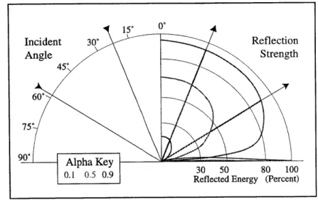
and 50% relative humidity. . . . 23 2-4 Angle dependent surface reflection plots for three materials with average

absorption coefficients of 0.9 (blue,) 0.5 (green,) and 0.1 (red.) . . . 24

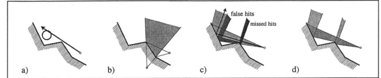
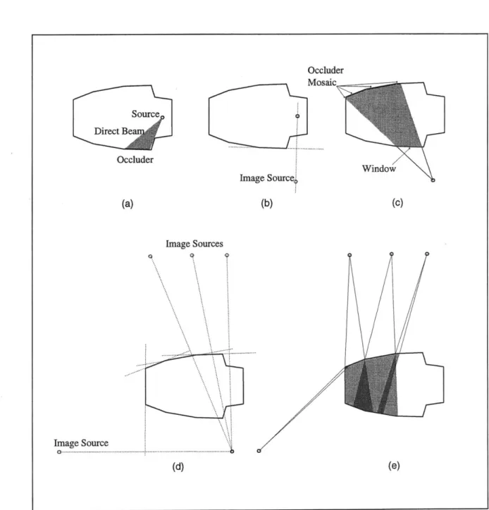
3-1 a) Ray tracing: positional errors. b) Image-source: limited scope of image source. c) Beam tracing with fixed profiles: false and missed hits. d) Gen-eral beams: correct hits. . . . .. . . -31 4-1 Graphical icons representing (from left to right): IACC, EDT, and BR. . . . 39 4-2 Scalar values of sound level data are represented with color over all surfaces

of an enclosure. . . . .. . . .. - - - -. 41 4-3 Visualization showing scalar values of sound level data represented with

color for the seating region along with EDT and BR values, represented with icons at a grid of sample points within an enclosure. . . . 41 4-4 Color indicates sound strength data at four time steps. . . . 42 5-1 Construction series for three generations of beams. Occluders are shown

in red, and windows are shown in green. Dotted lines indicate construction lines for mirrored image source location. . . . 45

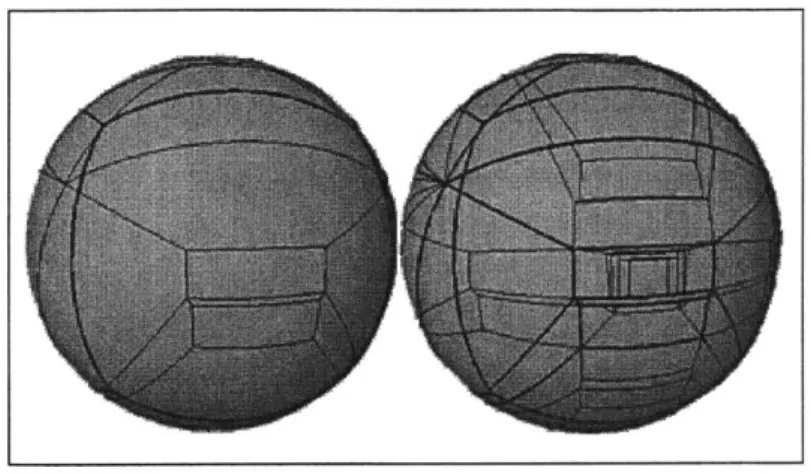
5-2 Beam profiles mapped onto a sphere centered at the source. a) First

gener-ation. b) Second genergener-ation. . . . 46

5-3 Receiver point within a beam projects onto the window and an occluder. . . 47

5-4 Improved energy decay calculation based upon projected areas, effective a. 48 5-5 Sphere with radius ri has the same volume V as the enclosure. Sphere with radius r2 has volume V2, twice the volume of the enclosure. The statistical time when a typical receiver will have incurred n hits is Ir. . . . 49

5-6 Hits from beams are combined with the statistical tail. . . . 51

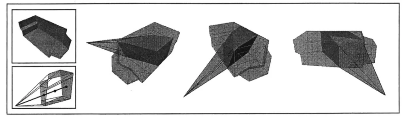
5-7 Octree representation of a beam intersected with a 3D receiver. . . . 52

5-8 Three snapshots of wave front propagation. . . . 54

5-9 Tempolar plots for three hall locations. . . . 55

7-1 Overview of the interactive design process. . . . 62

7-2 Material and geometry editors. . . . 64

7-3 Geometry constraint specification. a) Coordinate system axis icon used for transformation specification. b) Rotation constraint specified by orienting and selecting a rotation axis. c) Possible configurations resulting from trans-lation constraint specification for a set of ceiling panels. d) Scale constraint specified by indicating a point and direction of scale. The constraints are discretized according to user specified divisions . . . 65

7-4 Graphical difference icons representing (from left to right) IACC, EDT,and BR. ... ... . . . . . - . - - - - -. 66

7-5 Sound strength target specification. . . . 67

7-6 Sound level specification editor. . . . 68

7-7 These illustrations show ideal values for two different types of hall uses. left: symphonic music. right: speech. . . . 69

8-1 Interior photograph of Oakridge Chapel (courtesy of Dale Chote.) . . . 75

8-3 Computer model of Kresge Auditorium. . . . . 80 8-4 Variable positions for the rear and forward bank of reflectors and the back

stage wall in Kresge Auditorium for the initial (red) configuration, the ge-ometry only (green) configuration, and the combined materials and geom-etry (blue) configuration. . . . 82 8-5 Jones Hall: illustration of hall configuration with movable ceiling panels

(top) in raised position, and (bottom) in lowered position. Source of fig-ures: [25] . . . .. . -. . . . . 87

8-6 Computer model of Jones Hall. The left illustration shows the variable

po-sitions for the rear stage wall, and the right illustration shows the variable positions for the ceiling panels. The initial positions are indicated in red. . . 88

8-7 Resulting ceiling panel configurations for Jones Hall: left: symphony con-figuration (green,) right: opera concon-figuration (blue.) . . . 90

List of Tables

8.1 Acoustic measure readings for Oakridge Chapel. . . . 76

8.2 Acoustic measure readings for Kresge Auditorium. . . . 81

8.3 Acoustic measure readings for Jones Hall. The modified configuration en-tries give the individual objective ratings for the configuration resulting from the optimization using the combined objective. . . . .. . . 89

B.1 Acoustic measure targets for predefined objectives. . . . 103

C. 1 An example of a Material Library. . . . 105

D. 1 Ceiling variable assignments for Oakridge Bible Chapel. . . . 107

D.2 Wall and ceiling variable assignments for Oakridge Bible Chapel. . . . 108

D.3 Acoustic measure readings and objective function values for Oakridge Bible Chapel. . . . .. . .. . .. . - - - . .. 108

D.4 Initial materials for Kresge Auditorium. . . . 109

D.5 Variable assignments for the 'Material Only' optimization of Kresge Audi-torium . . . . - -. . - - - -. . . . 109

D.6 Variable assignments for the 'Material and Geometry' optimization of Kresge Auditorium . . . . - - - . . 110

D.7 Variable assignments for the 'Music' optimization of Kresge Auditorium. 110 D.8 Variable assignments for the 'Speech' optimization of Kresge Auditorium. 110 D.9 Acoustic measure readings and objective function values for Kresge Audi-torium . . . - . . . . . . - - - . 111

D. 10 Initial materials for Jones Hall. . . . 112 D. 11 Variable assignments for the combined objective for Jones Hall. . . . 112 D. 12 Acoustic measure readings and objective function values for Jones Hall. . 113

Chapter 1

Introduction

Acoustic design is a difficult process, because the human perception of sound depends on such things as decibel level, direction of propagation, and attenuation over time, none of which are tangible or visible. This makes the acoustic performance of a hall very difficult to anticipate. Furthermore, the design process is marked by many complex, often conflict-ing goals and constraints. For instance, financial concerns might dictate a larger hall with increased seating capacity, which can have negative effects on the hall's acoustics, such as excessive reverberation and noticeable gaps between direct and reverberant sound; fan shaped halls bring the audience closer to the stage than other configurations, but they may fail to make the listener feel surrounded by the sound; the application of highly absorbent materials may reduce disturbing echoes, but they may also deaden the hall. In many renova-tions, budgetary, aesthetic, or physical impediments limit modificarenova-tions, compounding the difficulties confronting the designer. In addition, a hall might need to accommodate a wide range of performances, from lectures to symphonic music, each with different acoustic re-quirements. In short, a concert hall's acoustics depends on the designer's ability to balance many factors.

In 1922, the renowned acoustic researcher, W. C. Sabine, had the following to say about the acoustic design task:

The problem is necessarily complex, and each room presents many conditions, each of which contributes to the result in a greater or less degree according to circumstances. To take justly into account these varied conditions, the solution of the problem should be quantitative, not merely qualitative; and to reach its highest usefulness it should be such that its application can precede, not follow, the construction of the building. [45]

Various tools exist today to assist designers with the design process. Traditionally, de-signers have built physical scale models and tested them visually and acoustically. For ex-ample, by coating the interiors of the models with reflective material and then shining lasers from various source positions, they try to assess the sight and sound lines of the audience in a hall. They also might attempt to measure acoustical qualities of a proposed environment by conducting acoustic tests on a model using sources and receivers scaled in both frequency and size. Even water models are used sometimes to visualize the acoustic wave propaga-tion in a design. These tradipropaga-tional methods have proven to be inflexible, costly, and time consuming to implement, and are particularly troublesome to modify as the design evolves. They are most effectively used to verify the performance of a completed design, rather than to aid in the design process.

The advent of computer simulation and visualization techniques for acoustic design and analysis has yielded a variety of approaches for modeling acoustic performance [12, 22, 34,

39, 13]. While simulation and visualization techniques can be useful in predicting

acous-tic performance, they fail to enhance the design process itself, which still involves a bur-densome iterative process of trial and error. Today's CAD systems for acoustic design are based almost exclusively on direct methods-those that compute a solution from a com-plete description of an environment and relevant parameters. While these systems can be extremely useful in evaluating the performance of a given 3D environment, they involve a tedious specify-simulate-evaluate loop in which the user is responsible for specifying input

parameters and for evaluating the results; the computer is responsible only for computing and displaying the results of these simulations. Because the simulation is a costly part of the loop, it is difficult for a designer to explore the space of possible designs and to achieve specific, desired results.

An alternative approach to design is to consider the inverse problem-that is, to allow the user to create a target and have the algorithm work backward to establish various pa-rameters. In this division of labor, the user is now responsible for specifying objectives to be achieved; the computer is responsible for searching the design space, i.e. for selecting parameters optimally with respect to user-supplied objectives. Several lighting design and rendering systems have employed inverse design. For example, the user can specify the lo-cation of highlights and shadows [42], pixel intensities or surface radiance values [47, 43], or subjective impressions of illumination [28]; the computer then attempts to determine lighting or reflectance parameters that best match the given objectives using optimization techniques. Because sound is considerably more complex than light, an inverse approach appears to have even more potential in assisting acoustic designers.

In this thesis, I present an inverse, interactive acoustic design system. With this ap-proach, the designer specifies goals for acoustic performance in space and time via high level acoustic qualities, such as "decay time" and "sound level." Our system allows the de-signer to constrain changes to the environment by specifying the range of allowable material as well as geometric modifications for surfaces in the hall. Acoustic targets may be suitable for one type of performance, or may reflect multiple uses. With this information, the sys-tem performs a constrained optimization of surface material and geometric parameters for a subset of elements in the environment, and returns the hall configuration that best matches performance targets.

Our audioptimization design system has the following components: an acoustic evalu-ation module that combines acoustic measures calculated from sound field data to produce a rating for the hall configuration; a visualization toolkit that facilitates an intuitive assess-ment of the complex time-dependent nature of sound, and provides an interactive means to

express desired acoustic performance; design space specification editors that are used to in-dicate the allowable range of material and geometry modifications for the hall; an optimiza-tion module that searches for the best hall configuraoptimiza-tion in the design space using both sim-ulated annealing for global searching and steepest descent for local searching; and a more geometrically accurate acoustic simulation algorithm that quickly calculates the sound field produced by a given hall configuration.

This system helps a designer produce an architectural configuration that achieves a de-sired acoustic performance. For a new building, the system may suggest optimal configu-rations that would not otherwise be considered; for a hall with modifiable components or for a renovation project, it may assist in optimizing an existing configuration. By using op-timization routines within an interactive application, our system reveals complex acoustic properties and steers the design process toward the designer's goals.

1.1 Thesis Overview

The remainder of this thesis is organized as follows. Chapter 2 provides background in room acoustics. Chapter 3 presents previous research in acoustic simulation algorithms. I survey sound characterization measures in Chapter 4 and present visualization tools used to display these acoustic qualities. Chapter 5 details our new simulation algorithm that addresses both computation speed and geometric accuracy. Chapter 6 defines the new components intro-duced by the inverse design approach-the specification of the design space, the definition of the objective function, and the optimization strategy used to search the design space for the best configuration. I describe the implementation details of these new components in the context of our audioptimization design system in Chapter 7. I demonstrate the audiop-timization system through several case studies of actual buildings in Chapter 8.

Chapter 2

Acoustics

This chapter presents background on the phenomenon of sound, from both a physical and psychological viewpoint. In addition, room acoustics is introduced, and a short survey of position independent acoustic measures is presented. Given this background information, the limitations of the approximations and simplifying assumptions made by the acoustic evaluation and simulation algorithms presented in the following chapters can be better un-derstood.

2.1 Physics of Sound

Sound is the result of a disturbance in the ambient pressure, Po, of particles within an elastic medium that can be heard by a human observer or an instrument [8]. Since my focus is room acoustics, I will be addressing sinusoidal sources propagating sound waves through air. As a sound wave travels, its energy is transferred between air particles via collisions. The result is a longitudinal pressure wave composed of alternating regions of compression and rarefac-tion propagating away from the source. Although the wave may travel a great distance, the motion of particles remains local, as particles oscillate about their ambient positions rela-tive to the wave propagation direction. While each particle will undergo the same motion, the motion will be delayed, or phase shifted, at different points along the wave. Particle

wavelength (one cycle) Maximum Compression amplitude AmbientAAA I Pressure _Distance Maximum cycles Rarefaction frequency '0 = second

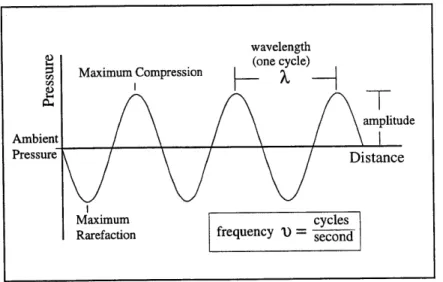
Figure 2-1: Wave terminology.

velocity u(t) and sound pressure p(t) are orthogonal, cyclic functions such that when par-ticle density is greatest, parpar-ticle velocity is at its ambient level, and when parpar-ticle velocity is greatest, particle density is at its ambient level [8].

Sound waves share the same characterization as waves of other types, summarized briefly as follows [20]. The length of one cycle of a sound wave-the distance between correspond-ing crest points, for example-is its wavelength, A, shown in Figure 2-1. The time it takes for the wave to travel one wavelength, is its period, T. Its frequency, v, is the number of cycles generated by the sound source in one second, measured in Hertz (Hz). The speed of sound c is independent of A, but depends on environmental conditions such as air tempera-ture, humidity, and air motion gradients. I assume static conditions for all acoustic modeling presented in this thesis, setting the speed of sound to 345 meters per second.

When the displacement of air by a disturbance takes place fast enough, that is, so fast that the heat resulting from compression does not have time to dissipate between wave cy-cles, the phenomenon is called adiabatic compression, and produces sound waves [8]. The resulting pressure change is related to the change in volume given by the equation PV" =

constant, where the gas constant -y is 1.4 for air. Under these adiabatic conditions, the

by the wave equation

02p

2

ap

1

82p

+

ar2 r ogr C2 19t2 with a solution of the form

p(r, t) = V2 p, (2.2)

where p, is the complex root mean square (rms) pressure at a distance r from the source, and

j is defined as v/-T [8]. This solution yields the (rms) pressure, or effective sound pressure, which monotonically decreases through time, not the instantaneous pressure, which is an oscillating function.

Intensity, I, is defined as the average rate at which power flows in a given direction through a unit area perpendicular to that direction. The relation between intensity and ef-fective sound pressure is given by

I = , (2.3)

where po is the density of air and c is the speed of sound, and the product po c is the charac-teristic impedance of the medium [8]. For a spherical source, intensity in the radial direction can also be expressed in terms of source power W, neglecting attenuation due to intervening media, as follows:

W

I= . (2.4)

4 7rr2

The audible range of sound for the typical human observer encompasses frequencies between 20 Hz and 20 kHz [20]. The perceptible range of intensity covers fourteen orders of magnitude [18]. Instead of working with intensity values directly, it is more convenient to convert these values to various log scale measures. These measures typically use decibel (dB) units, where a decibel is ten times the log of a ratio of energies. Intensity Level (IL) is given in decibels and is defined as

IL = 10 log , (2.5)

Iref

where Iref is 10-12,1"1, the weakest sound intensity perceptible to the typical human lis-tener [8]. A similar measure, Sound Pressure Level (SPL) is also given in decibels and de-fined as

SPL = 20 log -, (2.6)

Pref

where pref is 2 * 10-5n'2"" [8].

While these measures do not directly map to the human perception of loudness-a dou-bling of the sound level does not correspond to a doudou-bling of the perception of loudness-a

10 dB increase in level roughly maps to a doubling in loudness. In fact, a doubling of the

intensity of sound, or a 3 dB change in level, is just noticeable to the human observer [18]. Our perception of loudness is frequency dependent as well. A sound of 50 dB SPL will fall below our threshold of hearing at 50 Hz, while at 1 kHz it will be easily heard. Equal

loud-ness curves have been established that relate frequency and sound level to loudloud-ness [31]. Most sound sources produce complex sounds, composed of a rich spectrum of frequen-cies. As sound propagates throughout an enclosure, sound waves exhibit frequency depen-dent behavior. In the following sections we will take a look at the interaction of sound with surfaces in an enclosure, with intervening media, and with other sound waves, and discuss the role that frequency plays in these situations.

2.1.1

Sound Attenuation

Many aspects of our perception of sound within an enclosure are directly related to its decay through time. As it propagates, a spherical wave decays in intensity due to distance, air, and surface attenuation, as follows:

* Distance Attenuation: As can be seen from Equation 2.4, intensity decays with the

Figure 2-2: Distance attenuation obeys inverse-square law.

distributed over a larger area. Figure 2-2 shows this relationship.

e Air Attenuation: Sound intensity also decays by absorption as the sound wave passes through air. While this effect is negligible over short distances under normal atmo-spheric conditions, it is more significant in large acoustic spaces like concert halls and auditoria. The effect of air absorption on sound intensity is modeled by the following equation

I = Io * ed, (2.7)

where d is distance traveled in meters, and m is the frequency dependent energy at-tenuation constant in meters-' [8]. The value of m depends on atmospheric condi-tions such as relative humidity and temperature. Air attenuation is more pronounced for higher frequency sound. For example, after traveling a distance of 345 meters, (one second), the intensity of a 2 kHz wave will decrease roughly 43%, while that of a 500 Hz wave will decrease only 15% under certain atmospheric conditions. In this work, we fix the values for temperature at 680F and relative humidity at 50%.

atmo-Figure 2-3: Air attenuation curves for three frequencies of sound at room temperature and 50% relative humidity.

spheric conditions.

e Surface Attenuation: Surface absorption has the most significant effect on sound de-cay. Whenever a wave front impinges upon a surface, some portion of its energy is removed from the reflected wave. This sound energy is transferred to the surface by setting the surface into motion, which in turn may initiate new waves on the other side of the surface, accounting for transmission. The extent to which absorption takes place at a surface depends upon many factors, including the materials that comprise the surface, the frequency of the impinging wave front, and the angle of incidence of

the wave front.

The absorption behavior of a surface is commonly characterized by a single value, the

absorption coefficient, a, which is the ratio between energy that strikes the surface

and energy reflected from the surface, averaged over all incident angles [8]. While representing the behavior of sound reflecting from a surface with a single constant term only loosely approximates the actual behavior, it is a useful indicator of the effect that the surface will have on the overall acoustics of an enclosure. The non-uniformity of the reflection curves shown in Figure 2-4 gives an indication of the limitation of

Frequency Dependent Air Attenuation 0

25

50-751

100 1

Figure 2-4: Angle dependent surface reflection plots for three materials with average ab-sorption coefficients of 0.9 (blue,) 0.5 (green,) and 0.1 (red.)

this approximation method [35].

2.1.2 Wave Properties

If an obstacle is encountered whose surface is much more broad in dimension than the

wave-length of impinging sound, the surface will reflect the sound. The manner in which the sound is reflected depends upon the scale of surface roughness with respect to the wave-length of sound. Smooth surfaces will reflect sound geometrically, such that the reflection angle is equal to the angle of incidence. Surfaces with roughness of comparable or greater scale than the wavelength of sound will diffuse sound [31].

An obstacle whose scale is small compared to the wavelength of an approaching sound wave will have little effect on the wave. The wave will be temporarily disrupted after pass-ing the obstacle, and reform a short distance beyond it. This behavior occurs because the air particles that carry the sound energy are moving in all directions, and will spread the wave energy laterally if unrestricted. This behavior is called diffraction, and accounts for related behaviors such as sound turning corners, or fanning out as it passes through openings [20]. If one imagines a volume of air space through which many sound waves pass-from

many different directions, covering a spectrum of frequencies-the particles within that air space respond to all sound waves at once. The human listener is able to separate and discern the effects on those particles due to different frequencies, imposing some level of order to the chaos. If waves of the same frequency are traveling in the same direction through that air space, they will either reenforce each other if they are in phase, or interfere destructively if they are out of phase. In the following section I begin to discuss the degree to which various properties of sound are taken into account in the context of room acoustics.

2.2

Room Acoustics

One goal of room acoustics is to predict various characteristics of the sound that would be produced in an acoustic enclosure, given a description of the room and a sound source. All the information required to characterize the room's acoustics is generated by computing the sound field created by such a source within that room. Theoretically the response of the room could be solved exactly using the wave equation, given the myriad boundary condi-tions as input. Practically, however, the complexities introduced by any but the simplest conditions make this calculation intractable. Additionally, even if practical, such a calcula-tion would yield far more informacalcula-tion than necessary to characterize the behavior of sound in the room to the level of detail that is useful [31].

Fortunately, much insight can be gained by considering various degrees of approxima-tion of the sound source and the room, and making simplifying assumpapproxima-tions about the be-havior of sound transport and sound-surface interactions. I summarize a few of the most simple, yet useful approximations below.

2.2.1 Reverberation: Sabine's Formula

For many years the only measure of the acoustic quality of a space was its reverberance, or the time it took for a sound to become inaudible after the source was terminated.

that the material qualities of various surfaces and objects in the room have on the reverber-ance of the room. While a researcher at Harvard University, Sabine was given the task of determining why the lecture room of the Fogg Art Museum had such poor acoustics, and to suggest modifications that would solve the problem.

Sabine observed that, while the room was modeled after its neighbor, the acousticly successful Sanders Theatre, the materials of the surfaces were very different, with Sanders faced with wood and the lecture room with tile on plaster. He conducted an experiment in which he measured the reverberation times for various hall configurations. When empty, the hall's reverberance measured 5.62 seconds. Sabine gradually added a number of cushions from Sanders Theatre, arranged throughout the room, taking additional measurements. The reverberation time was reduced by the addition of cushions, reaching a low of 1.14 seconds. Sabine then tested and catalogued a number of materials and fixtures (including people,) calculating the absorption characteristics of each with respect to that of the seat cushions used previously.

By fitting the data to a smooth curve, Sabine realized that the minor discrepancies would

vanish if reverberation was plotted against the total exposed surface area of the cushions, instead of the running length of cushions. From these and other experiments, Sabine arrived at a formula, derived empirically, to predict the reverberation time T of a room given its volume V in cubic feet and the total room absorption a in sabins within the room. A sabin is defined as one square foot of perfect absorption. His formula follows:

T = 0.05-, (2.8)

a

where the number of sabins is found by summation, over all surfaces S in the room, of the product of surface area S, and the absorption coefficient o, [18]. Just as a is frequency dependent, so too is T. While this formula does not account for the effects of such factors as the proximity of absorptive materials to the source, for example, Sabine himself noted that "it would be a mistake to suppose that ... [the position of absorption within the room] is of no consequence." [45]

2.2.2

Statistical Approximations

The rate of decay of sound density D in a room can be approximated by calculating sta-tistical averages of the room's geometry and material characteristics [8]. The two values needed are the mean time between surface reflections, and the average absorption at reflec-tion. From this data the envelope of decay due to surface absorption is calculated.

The first simplification is introduced by replacing the geometric description of the room with its meanfree path, d, defined as the average path length that sound can travel between

surface reflections. d is approximated by the formula

4V

d= -, (2.9)

where V is the volume of the room, and S is the total surface area within the room [8]. Given d, the mean time, t', between reflections is simply t' = d, where c is the speed of sound.

Complex absorption effects at each surface are replaced by the average absorption

co-efficient for the entire enclosure,

a, which is the weighted average of surface absorption

_ a1S+a2S2

+--+nSn

a

=

(2.10)

S

Absorption due to the contents of the room is accounted for by appending their absorption values to the numerator, although their additional surface area is typically neglected in the denominator [8].

Statistically speaking, the sound energy remaining after the first reflection at time t' is given by Dt, = Do(1 - a), and at time 2t' by D2t, = Do(1 - d)2. Beranek shows that

by converting from a discrete into a continuous formulation, the following function gives a

statistical approximation to the energy density remaining at any point in time:

He solves for the reverberation time T by rearranging this equation to isolate t, and substi-tuting 60 dB for the ratio of Do to Dt, arriving at the following formula:

60V

T = 0 (2.12)

1.085ca"

where a' is termed metric absorption units, and is defined as -S ln(1 -

a),

While these tools give us some indication of the character of the sound field created by a source within an enclosure, they are limited by the simplifying assumptions implicit in their derivations. Energy density is not uniform throughout the enclosure, due in part to the irregularity of geometry and the non-uniform distribution of absorptive material. Further, during the last few decades a number of acoustic measures have been developed, which re-quire more detailed information about the sound field than these calculations provide. The values for many of these measures vary for different positions throughout the hall, and re-quire directional and temporal data along with the intensity of sound for each passing wave-front. Fortunately, a variety of sophisticated simulation algorithms have been developed in recent years. In the following chapter I survey these algorithms and discuss their strengths and weaknesses.

Chapter 3

Survey of Acoustic Simulation

Approaches

In order to evaluate the acoustics of a virtual enclosure it is necessary to simulate the sound field it produces and extract the data required to calculate various acoustic measures. There has been a large amount of previous work in acoustic simulation [7, 31]. These approaches can be divided into five general categories: ray tracing [30], statistical methods [22], radiant exchange methods [34, 48, 52], image source methods [12], and beam tracing [21, 34, 19]. There are also a variety of hybrid simulation techniques, which typically approximate the sound field by modeling the early and late sound fields separately and combining the results [22, 34, 39]. I survey the major simulation algorithms below.

3.1 Ray Tracing

The ray tracing method propagates particles along rays away from the source, which reflect from the surfaces they strike. Ray information is recorded by the receivers that these rays encounter within the enclosure. Since the probability is zero that a dimensionless particle will encounter a dimensionless receiver point in space, receivers are represented as volumes instead of points. Because of this approximation, receivers may record hits from rays that

could not possibly reach them, as shown in Figure 3-la. Errors in the direction and arrival time of the sound will also result.

Another shortcoming of this method is the immense number of rays that are necessary in order to insure that all paths between the source and a receiver are represented. As an illustration, consider a receiver point represented with a sphere of radius one meter, located ten meters from the source in any arbitrary direction. At this distance, one must shoot about

600 rays, uniformly distributed, to insure that the receiver sphere is struck. Now consider

the case where we are interested in modeling sound propagation through one full second. Given that sound will travel 345 meters in that amount of time, one would need about 100 times as many rays to insure that a receiver at that distance would be hit. At this sampling density, however, our receiver at ten meters would be struck by 100 redundant rays, all repre-senting the same path to the source. The problem is compounded when considering that the projected angle of any given surface, not the receiver sphere, may determine the minimum density of rays. While ray subdivision may address some of these issues, no guarantees can be made that all paths will be found using ray tracing.

3.2 Statistical Methods

By relaxing the restriction that rays impinging upon a surface must reflect geometrically, and

exchanging the goal of finding all possible paths between sources and receivers for the goal of capturing the overall character of sound propagation, ray tracing techniques have been imbued with statistical behavior. Diffusion is modeled with this method by allowing rays to reflect from surfaces in randomly selected directions based upon probability distribution functions. Furthermore, instead of continuing to trace rays as their energy decreases, rays may be terminated at reflection with a probability based on the absorption characteristics of the reflecting surface. Diffraction effects might also be modeled using statistical methods, perhaps by perturbing ray propagation directions mid flight between reflections. While the range of behaviors that can be captured with statistical approaches is quite broad, its

appli-false hits

missed hits

a) b) c) d)

Figure 3-1: a) Ray tracing: positional errors. b) Image-source: limited scope of image source. c) Beam tracing with fixed profiles: false and missed hits. d) General beams: cor-rect hits.

cation might be better suited to modeling later sound, when the direction of propagation is less critical.

3.3 Radiant Exchange Methods

Recently, the radiant exchange methods used for modeling light transport have begun to be applied to acoustic modeling. Assuming diffuse reflection, the percent of energy that leaves one surface and arrives at another is calculated for all pairs of surfaces in a polygonalized environment. Energy is then radiated into the environment, and a steady state solution is cal-culated. Two issues emerge when applying this technique to sound transport. First, while the arrival time can be ignored for light, it is critical for sound. Second, the diffuse reflection assumption is invalid for modeling most interactions between sound and surfaces. It is par-ticularly troublesome for modeling early sound, where the directional effects are especially important. While it is more acceptable to model late sound than the early sound using dif-fuse reflection assumptions, more cost effective approaches may suffice for modeling late

3.4 Image Source

The image source method is based on geometric sound transport assumptions. In the ideal case, the approach works as follows. In a room where the surfaces are covered with per-fect mirrors, a receiver would be afper-fected by every image of the source, whether direct or reflected, that is visible at the receiver location. No temporal or directional errors would result. While this is the ideal outcome, problems arise in the implementation of the method. Image sources are constructed by mirror reflecting the source across all planar surfaces, as shown in Figure 3-1c. This process recurses, treating each image source as a source. Each resulting image source could potentially influence each receiver. Unfortunately, many im-age sources constructed in this way are not realizable, and the valid ones are often extremely limited in their scope, as shown in Figure 3-1b. That is, they may only contribute to a frac-tion of the entire room volume. Recursive validity checking is required to ensure receiver-source visibility. Unless preemptive culling is performed during the construction of image sources, a geometric explosion of image sources results.

3.5

Beam Tracing

A variation on the ray tracing method is beam tracing. Here the rays are characterized by

cir-cular cones or polygonal cones of various preset profiles [57]. Receivers are represented as points. As these beams emanate from the source, receivers that are enclosed within the vol-ume of the beam are updated. As they propagate, beams reflect geometrically from surfaces encountered by their central axis. The geometric explosion that characterizes the image source method is avoided here because the number of beams does not grow during propaga-tion. However, the method suffers from various shortcomings. If circular beams are packed such that they touch but do not overlap each other, then gaps result, leaving regions within the room erroneously uneffected by the sound. Conversely, if the beams are allowed to over-lap, removing the gaps, then regions are double covered, causing simulation errors [33]. These systematic errors are eliminated for the direct field by using perfectly packed

trian-gular profiles, for example, which attain full spherical coverage of the source. However, the errors reemerge at reflection since beams are not split when they illuminate multiple surfaces, striking an edge or a corner. As a consequence, false hits and missed hits result,

as shown in Figure 3-lc [34].

3.6 Hybrid Methods

Many hybrid approaches have emerged that incorporate the best features of these methods. The image source method is best used for modeling early reflections where directional and temporal accuracy is critical. The method may be paired with ray tracing, which is used to establish valid image sources [39, 58]. The image source method is rarely used for later reflections due to the exponential increase in cost. Lewers models late sound with the radi-ant exchange method [34]. Others use ray tracing, randomizing the reflection direction to attain a diffusing effect [39]. Still others use a statistical approach based on the results of an earlier, or ongoing ray tracing phase [57, 22]. Heinz presents an approach in which surfaces in the enclosure are assigned a wavelength dependent diffusion coefficient, which is used to transfer energy from the incoming ray to the diffuse field [22]. Various approaches are used to combine the early and late response simulations.

3.7 Summary

In the context of acoustic design, it is not necessary that the simulations achieve audio-realistic results. In fact, such a level of detail would detract from the process. While the

high computation costs required by radiant exchange methods may be worthwhile for ap-plications requiring high fidelity reproduction, geometric assumptions suffice for our pur-poses. In Chapter 5 1 describe our new acoustic simulation algorithm, which builds upon the strengths of the methods just described, making improvements in both geometric accuracy and computation speed. In addition, I present a more complete set of acoustic performance

Chapter 4

Acoustic Evaluation

This chapter presents the set of objective measures used by our system to evaluate the acous-tic quality of a performance space. I define the measures in the first section and introduce visualizations of the measures in the second section. These visualizations and associated in-teractive tools give the user of the system an intuitive way to quickly assess acoustic quality.

4.1 Characterization of Sound

Traditionally, reverberation time and other early decay measurements were considered the primary evaluation parameters in acoustic design. However, in recent years, researchers have recognized the inadequacies of using these criteria alone and have introduced a vari-ety of additional measures aimed at characterizing the subjective impression of human lis-teners [7]. For example, in 1991 Wu applied fuzzy set theory, noting that the subjective response of listeners is often ambiguous [63]. In 1995, Ando proposed another approach showing how to combine a number of orthogonal objective acoustic measures into a sin-gle quality rating using his subjective preference test results [5]. In 1996, Beranek built on Ando's work by linearly combining six statistically independent objective acoustic mea-sures into an evaluation function that gives an overall acoustic rating [10]. In this research, we employ Beranek's evaluation approach, known as the Objective Rating Method (ORM).

Below I define the six acoustic measures and introduce visualization techniques used to evaluate them.

Interaural Cross-Correlation Coefficient (IACC). The Interaural Cross-Correlation

Co-efficient is a binaural measure of the correlation between the signal at the two ears of a lis-tener. It characterizes how surrounded a listener feels by the sound within a hall. If the sound comes from directly in front of or behind the listener, it will arrive at both ears at the same time with complete correlation, producing no stereo effect. If it comes from an-other direction, the two signals will be out of phase and less correlated, giving the listener the desirable sensation of being enveloped by the sound. I use the following expression to calculate IACC from computer simulated output [5]:

IACC = ( A2(P) 2j)(P) (4.1)

where I( is the interaural cross correlation of the pth pulse, (D') and i$() are the autocorre-lation functions at the left and right ear, respectively, and A, is the pressure amplitude of the pth pulse from the set of P pulses. The correlation values depend on the arrival direction of the wave with respect to the listener's orientation. The numerator is greater for highly cor-related frontal signals than for less corcor-related lateral signals. Since the amplitude of sound decreases rapidly as it propagates, the sound waves that arrive the earliest generally have far greater effect on IACC.

Early Decay Time (EDT). The Early Decay Time measures the reverberation or liveliness

of the hall. Musicians characterize a hall as "dead" or "live," depending on whether EDT is too low or high. The formal definition of EDT is the time it takes for the level of sound to drop 10 decibels from its initial level, which is then normalized for comparison to traditional measures of reverberation by multiplying the value by six. As Beranek suggests, I determine

EDT by averaging the values of EDT for 500 Hz and 1000 Hz sound pulses. The best values

Bass Ratio (BR). The Bass Ratio measures how much sound comes from bass, reflecting the

persistence of low frequency energy relative to mid frequency energy. It is what musicians refer to as the "warmth" of the sound. BR is defined as:

BR = RT1 25 + RT250 (4.2)

RT500 + RT1000'

where RT is the frequency dependent reverberation time. RT is the time it takes for the sound level to drop from 5 dB to 35 dB below the initial level, which is then normalized for comparison to traditional measures of reverberation by multiplying by two. For example, for a 100 dB initial sound level, RT would be the time it takes to drop from 95 dB to 65 dB multiplied by the normalizing factor. The ideal value of BR ranges between 1.1 and 1.4 for

concert halls.

Strength Factor (G). The Strength Factor measures sound level, approximating a general

perception of loudness of the sound in a space. It is defined as follows:

G = 10 log , (4.3)

(foo A (t)dt)

where t is the time in seconds from the instant the sound pulse is initiated, i(t) is the in-tensity of a sound wave passing at time t, and iA(t) is the free field (direct) inin-tensity ten meters from the source. The numerator accumulates energy from the pulse as each prop-agated wave passes a receiver, until it is completely dissipated; the denominator receives only a single energy contribution. The division cancels the magnitude of the source power from the equation, allowing easy comparison of measured data across different halls. I av-erage the values of G at 500 Hz and 1000 Hz. The preferred values for G range between 4.0

dB and 5.5 dB for concert halls. In general, G is higher at locations closer to the source. It is instructive to see how the sound level changes through time, as well as location. We perceive a reflected wave front as an echo-perceptibly separable from the initial sound-if it arrives more than 50 msec. after the direct sound and it is substantially stronger than its neighbors. The time distribution of sound also affects our perception of clarity. Two

locations in a hall may have the same value of G, but if the energy arrives later with respect to the direct sound for one location than the other, speech will be less intelligible, and music less crisp.

Initial-Time-Delay Gap (TI). The Initial-Time-Delay Gap measures how large the hall

sounds, quantifying the perception of intimacy the listener feels in a space. It depends purely on the geometry of the hall, measuring time delay between the arrival of the direct sound and the arrival of the first reflected wave to reach the listener. In order to make comparisons among different halls, only a single value is recorded per hall, measured at a location in the center of the main seating area. It is best if TI does not exceed 20 msec.

Surface Diffusivity Index (SDI). The Surface Diffusivity Index is a measure of the amount of sound diffusion caused by gross surface detail, or macroscopic roughness of surfaces within a hall. SDI is usually determined by inspection, and it correlates to the tonal quality of the sound in a hall. I compute the SDI index for the entire hall by summing the SDI as-signed to each surface material, weighted by its area with respect to the total surface area of the hall. SDI can range between 0.0 and 1.0, with larger values representing more diffusion. The preferred value of SDI is 1.0. For example, plaster has a lower index than brick, which

has a lower index than corrugated metal.

These six statistically orthogonal acoustic measures form the basis for our analysis and optimization work. While two of the measures, SDI and TI, are single values representing the entire hall, I compute the others by averaging the values sampled at multiple spatial po-sitions, and, in the case of G, multiple points in time. Refer to Appendix A for pseudocode describing the calculation of each measure.

4.2 Visualization of Acoustic Measures

Work has been done in representing sound field data with both visualizations and aural-izations. Stettner presented a set of 3D icons to graphically convey the behavior of sound

within an enclosure [50]. He also showed the accumulation of sound energy through time

by animating pseudo-colors applied to enclosure surfaces. The Bose Auditioner system [13]

provides auralizations from simulation data at specific listener positions within a modeled hall; these auralizations approximate what the hall might sound like. Our system provides visualizations for both the sound field and a collection of acoustic measures that describe the character of the sound field as it varies in space and time within an environment. These visualizations are used both to analyze the behavior of a given design and to interactively specify desirable performance goals. In this section, I describe these visualizations and

as-sociated interactive tools.

2 0 1.0 2.0mi

low

IACC= 0 EDT=r BR- low

1800 mid

Figure 4-1: Graphical icons representing (from left to right): IACC, EDT, and BR.

The six acoustic measures used to evaluate the quality of sound fall into three categories. The first group includes those measures calculated directly from the configuration of the enclosure, requiring no sound field simulation data. TI and SDI are in this category, and their values are displayed in a text field. Members of the second group share the characteristic that their values differ throughout the enclosure. The measures IACC, EDT and BR are of this type, and are represented using icons, as shown in Figure 4-1. The third type of measure is derived from data that not only contains a spatially varying component, but a temporal component as well. Sound Strength G is of this type.

When designing icons for IACC, EDT and BR, we tried to leverage the intuition of the user whenever possible to help convey meaning. We chose representations that would all be clear from the same view direction. A cylinder is placed at each listener position, or sample

point, upon which the icons are placed. A description of the visualization tool used for each measure in the second and third category follows.

" IA CC: IACC is represented as a shell surrounding the listener icon, which

illus-trates the degree to which the listener feels surrounded by the sound. The greater the degree of encirclement of the icon by the shell, the more desirable the IACC value. " EDT: EDT is represented graphically as a cone, scaling the radius by decay time

and fixing the height. The slope of the cone gives the viewer an intuition for the rate of decay of sound. For a value of 2.0, the cone is twice the width of the listener icon. " BR: Figure 4-1 shows the graphical icon we use for BR, composed of two stacked

concentric cylinders of different widths. The top cylinder represents the mid frequency energy and the bottom cylinder represents the low frequency energy. The height of each cylinder represents the relative values in the ratio, with constant combined height.

A listener icon representing a desirable BR value of 1.25 would have the top of the

lower cylinder just above the halfway mark, as depicted in the figure.

" G: The remaining view space real estate is utilized by using color to represent relative scalar values of sound level data, sampled over selected surfaces within the enclosure. The user may choose to view G over all surfaces, as shown in Figure 4-2, or over seating regions only, as in Figure 4-3. In the latter case, we include the ability to view the accumulation of sound level through time (see Figure 4-4), simply

by moving a slider. The sampling density over the seating regions is user controlled.

This feature gives the user another way to set the balance between the accuracy and speed of the acoustic simulation, as discussed at length in Chapter 5.

I have presented the set of objective acoustic measures used by our goal-based acoustic design system to evaluate the acoustic quality of a performance space, and I have described visualizations used to communicate their values. In the following chapter I will describe the simulation algorithms that generate the data required for the calculation of these acoustic measures.

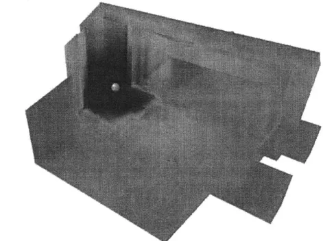
Figure 4-2: Scalar values of sound level data are represented with color over all surfaces of an enclosure.

Figure 4-3: Visualization showing scalar values of sound level data represented with color for the seating region along with EDT and BR values, represented with icons at a grid of sample points within an enclosure.

~TJ~I~ -~ - -~--- _ -

-10 msec 40 msec

80 msec 120 msec

Chapter

5

Acoustic Simulation: A Unified Beam

Tracing and Statistical Approach

In order to evaluate the acoustics of a virtual enclosure it is necessary to simulate the sound field it produces and extract the data required to calculate various acoustic measures. In this chapter, I introduce a new hybrid simulation algorithm [37] with two components: a sound beam generator that generalizes previous beam tracing methods for increased geo-metric accuracy [16], and a statistical approximation of late sound that leverages the beam tracing phase for increased speed. As with previous methods, I make a number of simpli-fying assumptions about sound transport, and replace the description of the enclosure with a planar representation. In the test models used in this thesis, this representation typically consists of a few dozen to a few hundred polygons.

I employ the geometric model of sound transport, which assumes that sound travels in

straight lines, and reflects geometrically from surfaces. Wave effects such as diffraction, de-structive interference, and other phase related effects are not considered. The angle depen-dent absorption characteristics of surfaces are not modeled, although frequency dependepen-dent characteristics are included.