HAL Id: hal-01672378
https://hal.archives-ouvertes.fr/hal-01672378
Submitted on 24 Dec 2017
HAL is a multi-disciplinary open access
archive for the deposit and dissemination of
sci-entific research documents, whether they are
pub-lished or not. The documents may come from
teaching and research institutions in France or
abroad, or from public or private research centers.
L’archive ouverte pluridisciplinaire HAL, est
destinée au dépôt et à la diffusion de documents
scientifiques de niveau recherche, publiés ou non,
émanant des établissements d’enseignement et de
recherche français ou étrangers, des laboratoires
publics ou privés.
Forecast scheduling and its extensions to account for
random events
Hind Zaaraoui, Zwi Altman, Eitan Altman, Tania Jimenez
To cite this version:
Hind Zaaraoui, Zwi Altman, Eitan Altman, Tania Jimenez. Forecast scheduling and its extensions
to account for random events. ICIN 2018 - 21st Conference on Innovation in Clouds, Internet and
Networks, Feb 2018, Paris, France. pp.1-8. �hal-01672378�
Forecast scheduling and its extensions to
account for random events
Hind Zaaraoui
∗, Zwi Altman
∗, Eitan Altman
†and Tania Jimenez
‡ ∗Orange Labs44 Avenue de la Republique, 92320 Chatillon, France Email:{hind.zaaraoui,zwi.altman}@orange.com
†INRIA Sophia Antipolis and LINCS, France
Email:[email protected]
‡Avignon University
Email:[email protected]
Abstract—Technology evolutions make possible the use of Geo-Localized Measurements (GLM) for performance and quality of service optimization thanks to the Minimization of Drive Testing (MDT) feature. Exploiting GLM in radio resource management is a key challenge in future networks. The Forecast Scheduling (FS) concept that uses GLM in the scheduling process has been recently introduced. It exploits long term time and spatial diversity of vehicular users in order to improve user throughputs and quality of service. In a previous paper we have formulated the FS as a convex optimization problem namely the maximization of an α−fair utility function of the cumulated downlink data rates of the users along their trajectories. This paper proposes an extension for the FS model to take into account different types of random events such as arrival and departure of users and uncertainties in the mobile trajectories. Simulation results illustrate the significant performance gain achieved by the FS algorithms in the presence of random events.a
Index Terms—Forecast scheduler, alpha-fair, high mobil-ity, Radio Environment Maps, geo-localized measurements, random events, trajectory uncertainty
I. INTRODUCTION
The use of GLM to improve network performance and profitability is receiving growing interest by network operators. The reason is threefold: First, it allows the operator to better know what is the real Quality of Service (QoS) provisioning to customers at any location (and not only at cell level). Second, it provides significant levers to optimize the network performance; and third, it allows personalized, user centric optimization. GLM can feed new Radio Resource Management (RRM) algo-rithms, Self-Organizing Network (SON) algoalgo-rithms, and in general, a management entity responsible to configure, optimize and troubleshoot the network. This view of
aThis work has been partially carried out in the framework of
IDEFIX project, funded by the ANR under the contract number ANR-13-INFR-0006.
GLM utilization corresponds to the general trend in 5G networks, namely the utilization of data from different sources in order to improve network operation. The data can feed applications on top of the Operation Support System such as a centralized SON server or directly feed virtual network functions in the virtual radio access network.
The perspective of having GLM has opened an active research and development domain, namely the construc-tion of Radio Environment Maps (REMs) using spatial interpolation techniques [1]. [2] for example utilizes coverage prediction algorithms based on geo-statistics Fixed Rank Kriging algorithm which is adapted to han-dle geo-location errors. The REM can be created and updated in a MDT server in the management plane and be downloaded into each Base Station (BS). It can provide maps for different quantities such as the received signal strength or Signal to Interference plus Noise Ratio (SINR). The BS can then use the REM to derive policies, to optimize different RRM algorithms such as association, handover or resource allocation, or manage interference and coverage problems. It is noted that in spite of the potential plethora of applications provided by REMs, most of the research has focused on the creation of the REM itself.
The capability of User Equipments (UEs) to report GLM to the network finds its roots in the introduction of MDT in the Long Term Evolution (LTE) standard [3]. The term MDT was motivated by the need to replace costly drive tests in order to manage and to troubleshoot the network using GLM generated by UEs. The MDT feature is presently available in mobile chipsets and can be activated by mobile operators.
The purpose of this paper is to design a scheduler, namely the FS that, by utilizing a REM, can benefit from long-term time-space diversity. The basic concept of the
FS has been introduced in [4] with application to data type of services. The FS allocation is formulated as a convex optimization problem, namely the maximization of an α−fair utility function of the cumulated rates of the mobile users along their trajectories. Similarly to the classical α−fair scheduling such as the Proportional Fair (PF) [5],[6], the forecast scheduler is an opportunistic scheduler with a degree of fairness depending on the choice of the α−fair parameter. However, the scheduling gain is not related to short term user diversity in fast fading states (measured in a millisecond timescale) as in classical α−fair scheduler, but to the long term user diversity along the trajectory. An important result of [4] that motivates the FS approach is its robustness to interference: The interference condition used to generate the REM with respect to the actual one experienced by the users has little impact on the scheduler decision, and negligible impact on the allocated rates.
Several contributions in the area of anticipatory or proactive scheduling have been recently repported (see for example [7] and references therein), with particular focus on video streaming applications. In [7], using the play-out buffer state and future channel states, the authors optimize spectral efficiency while avoiding or minimizing stalling durarion.
This paper generalizes the FS formulation to include random events such as arrivals and departures of users, or uncertainty in the predicted trajectories. The contribu-tions of the paper are the following:
• The α−fair concept is extended to the FS fairness, • A multiclass version of the FS is formulated,
• Heuristic solutions for the FS are developed to take into account random events such as users’ arrivals and departures and uncertainties in their trajectories. The paper is organized as follows: Section II recalls the basic FS model and shows how it extends the standard α−fair scheduling. Section III generalizes the FS model to the multiclass case, and proposes heuristic solutions to take into account random events. Numerical results for the different FS formulations are described in Section IV followed by concluding remarks in section V.
II. BASIC MODEL
In this Section we briefly recall the basic formulation of the FS as presented in [4]. Then, using Karush-Kuhn-Tucker (KKT) conditions, we show the relation between the FS and the α-fair scheduling.
A. Forecast scheduling formulation
Consider a macro-cell (BS) surrounded by interfering BSs. A REM is deployed in the BS and provides SINR values corresponding to the mobile location. It is recalled that a REM can provide the metric values (SINR in our case) at any point of the map thanks to interpolation algorithms, and hence any scheduling periodicity can be considered.
Consider n full buffer users moving at a constant speed during a time interval T - the scheduling period, over which n is considered constant. Suppose that time is in a discrete space: t ∈ {1, 2, .., T } = [|1, T |] and let i denote the user number, i ∈ {1, 2, .., n} = [|1, n|]. We suppose that during the scheduling duration there are no arrivals or departures of users (this assumption is later on relaxed).
A scheduling period T (typically of the order of sec-onds) is divided into scheduling time slots denoted here for simplicity as time units (e.g. of 1 ms), during which the bandwidth is shared among the scheduled users. Let ai(t) denote the bandwidth proportion allocated to a user
i at time t, ai(t) ∈ [0, 1], according to the scheduling
strategy, where ∀t, Pn
i=1ai(t) = 1, and W - the total
bandwidth. Using the Shannon equation, we write the throughput as a function φ of the SINR of user i as follows
ai(t)φ(SIN Ri(t)) = ai(t)W log2(1 + SIN Ri(t)). (1)
Denote by St
i the predicted SINR (i.e. the one provided
by the REM). The FS allocation policy is defined by the following optimization problem, with α 6= 1:
maximize : f (a) = n X i=1 (PT t=1ai(t)φ(Sit)) 1−α 1 − α (2) subject to : ∀i, ∀t, ai(t) ≥ 0 ∀t, n X i=1 ai(t) = 1
and for α → 1, the optimization problem with the same constraints reads: maximize : f (a) = n X i=1 log( T X t=1 ai(t)φ(Sit)). (3)
Both equations (2) and (3) have concave functions f for α ≥ 0, and can be solved using convex optimization. For example, one can use the convex optimization solvers such as CVX [8]. The size of the optimization problem is defined by the number of unknown variables, namely n × T .
The interpretation of (2) and (3) is the following: resources are shared fairly among the users according to the data-rate variation in their future trajectories. For example, if a user has a large enough coverage hole in his future trajectory, the forecast scheduler will take this into account and may allocate this user as much data as possible before reaching the coverage hole so as to remain fair with respect to the other users.
B. KKT for computing the FS
We briefly present the KKT optimality conditions for the forcast scheduling problem (2). It is known to provide necessary and sufficient optimality conditions. We have been using this approach to obtain closed form solutions in the special case of two users.
The objective and constraint functions in (2) are continuously differentiable for any a = (a1(1), ...a1(T ), a2(1), ..., an(T )) ∈ RnT, then
there exist multipliers λk,j and νj, where k ∈ [|1, n|]
and j ∈ [|1, T |], called KKT multipliers ([9], Chap.5) with the following Lagrangian function:
L(a, ν, λ) = f (a)+ T X j=1 νj( n X k=1 ak(j)−1)+ X k,j λk,jak(j), (4) where λk,j≥ 0.
We define the Lagrange dual function as the maximum value of L over a. Let a∗ maximize the Lagrangian function (4) for the optimal multipliers λ∗k,j and νj∗, where k ∈ [|1, n|] and j ∈ [|1, T |]. The gradiant at this point is null:
∇L(a∗, ν∗, λ∗) = 0 (5) hence for all i ∈ [|1, n|] and t ∈ [|1, T |] the following KKT conditions should be verified:
∂f (a) ∂ai(t) + ∂ ∂ai(t) T X j=1 νj( n X k=1 ak(j) − 1) + ∂ ∂ai(t) X k,j λk,jak(j) = 0, ai(t) ≥ 0, n X i=1 ai(t) = 1, λi,tai(t) = 0, λi,t ≥ 0, which is equivalent to : φ(Sit)( T X j=1 a∗i(j)φ(Sij))−α+ νt∗+ λ∗i,t = 0, (6) a∗i(t) ≥ 0, (7) n X k=1 a∗k(t) = 1, (8) λ∗i,ta∗i(t) = 0 (9) λ∗i,t ≥ 0. (10) We note that from (6), at any time t and for all users i and w, w 6= i we have φ(Sit)( T X j=1 a∗i(j)φ(Sij))−α+ λ∗i,t = φ(Swt)( T X j=1 a∗w(j)φ(Swj))−α+ λ∗w,t. (11) Similarly, from (6), for all user i and time t and u:
λ∗i,t+ νt∗ φ(St i) =λ ∗ i,u+ νu∗ φ(Su i) (12) since νt∗ does not depend on the users, and PT
j=1a ∗ i(j)φ(S
j
i) does not depend on time. Equality
(11) explicits the resource balancing among users at each time relative to α in the sense of equalizing the two expressions of each two users.
We deduce from (11) that the choice of α impacts the user selection:
• When α = 0, (11) is equivalent to φ(Sit) + λ∗i,t = φ(Swt) + λ∗w,twhich means that the scheduled user
at a future time t is the one who reaches the highest data rate at t due to equation (9). Interestingly, this particular case is the same as the normal α-fair scheduling since the maximum of the sum in the utility function is the sum of the maximum in this case.
• When α −→ 1 the FS becomes the forecast
propor-tional fairscheduler.
• When α −→ ∞ the FS becomes the max-min
forecast fairness scheduler.
Consider the case where an optimal policy uses a∗i > 0 for all i in some set I∗ and uses a∗w = 0 for w /∈ I∗.
Then for all i, k ∈ I∗ and w /∈ I∗, and by (9) that states
that λ∗i,t = 0 we have
φ(St i) (PT j=1a∗i(j)φ(S j i))α = (13) φ(St k) (PT j=1a∗k(j)φ(S j k))α = φ(S t w) (PT j=1a∗w(j)φ(S j w))α + λ∗w,t.
Since λw,t≥ 0, we have φ(St i) (PT j=1a ∗ i(j)φ(S j i))α ≥ φ(S t w) (PT j=1a∗w(j)φ(S j w))α .
The above formulation suggests a solution using a water filling type algorithm for this problem, and has enabled us to obtain an explicit solution for the special case of two users only.b
III. MULTICLASS AND RANDOM EVENTSFS
PROBLEMS
This Section generalizes the optimization model (2) in order to take into account arrivals and departures of users as well as different classes of users such as fixed and mobile, real time and non-real time services or users having different random trajectories.
A. Multiclass problem
Denote by C1 the set of real-time active users and
by C2- the set of non-real time (elastic) users. Let T1
be the minimum scheduling period for a real time user. T2 is the FS duration for all users in class C2, which
is subdivided into minimum scheduling periods of T1
(namely T2>> T1).
Static or low speed users can be included in the set C1 where users can benefit from fast fading. It is
noted that if service differentiation is sought, weighting coefficients ws(i)(s(i) being the service of the user i) can
be introduced as in Weighted Fair Queueing scheduling. The new FS model including the real-time class is written follows: maximize : f (a) = X i∈C2 (Pm t=1ai(t)φ(S t i))1−α 1 − α + X i∈C1 m X t=1 ws(i) (ai(t)φ(Sti)) 1−α 1 − α (14) subject to : ∀i, ∀t, ai(t) ≥ 0 ∀t, X i∈C1∪C2 ai(t) = 1 where m = T2/T1.
We can have as many classes as types of users and types of trajectories. For example, users approaching a traffic junction with a distance below d are attributed to a new class, denoted as C3 in Fig.1. The corresponding
duration T3 for users in C3, T3 < T2, is defined
as a function of d. The corresponding term added to the objective function of the optimization problem (14)
bResearch report in preparation.
during the period T3 is denoted as Restricted Forecast
Scheduling (RFS). At the end of T3, the users arriving
next to the random point with a distance less than d to it are switched to the set C1 due to both lower speed
and trajectory uncertainty (users can turn left, right or continue straight, see Fig.1).
Fig. 1. Forecast scheduling with different classes of traffic
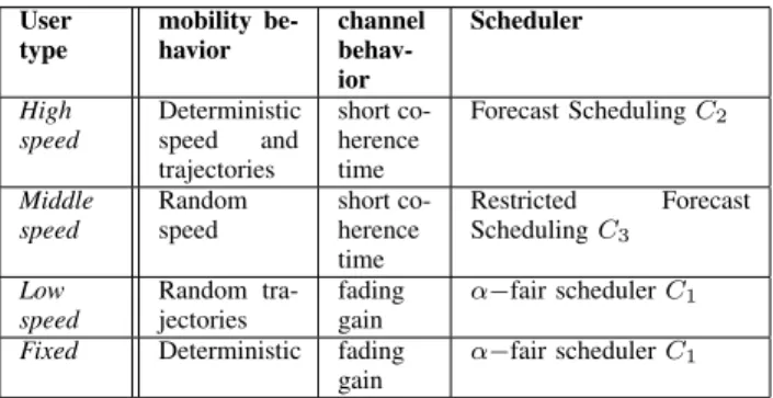
Table I summarizes the types of schedulers with the corresponding types of mobility and channel behaviours.
TABLE I
SCHEDULING TYPES WITH THE CORRESPONDING TYPES OF
MOBILITY AND CHANNEL BEHAVIOURS
User type mobility be-havior channel behav-ior Scheduler High speed Deterministic speed and trajectories short co-herence time Forecast Scheduling C2 Middle speed Random speed short co-herence time Restricted Forecast Scheduling C3 Low speed Random tra-jectories fading gain α−fair scheduler C1
Fixed Deterministic fading gain
α−fair scheduler C1
B. Arrivals and departures problem
The extension of the optimization model (2) to include arrivals and departures is described presently. One can make the same extension for the optimization problem (14). New users can be integrated in the set C1 at each
arrival time, however they will not benefit from the FS. A heuristic solution consists of initializing the opti-mization problem (2) or (14) at each user arrival and
departure. To remain fair among all users, including those who have not yet been scheduled, we recompute the forecast scheduler at each event, taking into account the received past data. This new heuristic scheduling solution is denoted the Updated Forecast Scheduling (UFS) and is inspired by the rolling horizon approach [10]. It is noted that optimizing the problem (2) or (14) for each time step or for each random event occurrence time (random variation of speeds, trajectories, number of users), taking into account the received past data, gives the same result, however the latter has significant lower complexity.
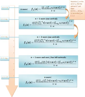
When restarting the scheduling algorithm, it is im-portant to reinject the data already received in the last scheduling period in order to remain fair among all users. In Fig.2 we explicit the scheduling algorithm for the particular optimization problem (2):
1) At time t = 1 we maximize the function f of the optimization problem (2) denoted by f1 over the
period T ;
2) We find b1= (b11(1), ..., b11(T ), ..., b1n(1), ..., b1n(T ))
the optimal solution of the function f1;
3) For the first event (arrival for example) at time t = u2, we replace ai(1), ..., ai(u2 − 1) by
b1
i(1), ..., b1i(u2− 1) for all users i in the function
f1. We obtain a new function f2to optimize at time
t = u2 (see Fig.2).
4) We proceed iteratively with the optimization of fN
at the event number N − 1 for N ∈ [1, T ]:
fN(a) = n X i=1 (PuN−1 t=1 b t i(t)φ(Sit) 1 − α + PT t=uNai(t)φ(S t i)) 1−α)1−α 1 − α (15)
IV. NUMERICAL RESULTS
We present in this Section the numerical simulations obtained using a Matlab simulator. Users are moving with a speed of 50 km/h. It is recalled that at this speed, due to too short coherence time, one cannot exploit fast fading to achieve opportunistic scheduling gain. For this reason we consider the Round Robin (RR) as a base line to the different approaches. The spatial resolution of the REM is of 1m (it is recalled that the REM interpolates GLM), and in 50km/h it corresponds to a 70 ms time intervals over which the SINR is considered constant. Hence the time resolution of the FS is of 70 ms. During this time interval, a fixed allocation is applied, namely the same users are scheduled at a time interval depending on the technology (e.g. 1 ms for LTE).
Fig. 2. FS algorithm taking into account arrival and departure of users
In the scenarios considered in this Section, a Virtual Small Cell (VSC), namely a remotely created small cell using a Large Scale Antenna System (LSAS) [11] is considered to enhance spatial SINR diversity along the trajectory.
A. CVX resolution
The objective function of the optimization problem (2) is a convex function that calls for convex optimization solver. The CVX library implemented in Matlab to re-solve this kind of problems has been used (see [8] and [12]). The CVX resolution process verifies the convexity of the problem and solves it using SDPT3 or SeDuMi. SDPT3is a MATLAB implementation of infeasible path-following algorithms for solving conic programming problems whose constraint cone is a product of semidefi-nite cones. It uses a predictor-corrector primal-dual path-following method, with different types of search direc-tion. SeDuMi is a linear/quadratic/semidefinite solver for Matlab and Octave.
Simulation parameters are depicted in Table II. B. FS with randomness
Two different types of randomness are studied in the following: trajectory randomness and a user arrival in
TABLE II
NETWORK ANDTRAFFIC CHARACTERISTICS
Network parameters
Number of macro BSs 1
Number of interfering BSs 6
Macro-cell layout hexagonal omni sectors Intersite distance 500m
Bandwidth 20M Hz
Channel characteristics
Thermal noise −174dBm/Hz
Macro Path loss (d in km) 128.1 + 37.6 log10(d) dB
Mobility traffic characteristics
User speed 50km/h
Number of users 10
File size σ full buffer (∞) One iteration = Scheduling delay 70ms
the network. We analyze the impact of a random event occurrence on five types of schedulers:
• The basic FS which does not take into account any random event during the scheduling duration T (section II-A);
• UFS which stops at each random event occurrence and integrates the past data allocated by the FS before reiterating (Section III-B);
• RFS which stops at T0 < T and integrates the
past data allocated by the FS before reiterating. This scheduling is usefull when we know when the random event will occur (any randomness along the trajectories such as a crossroad) (section III-A);
• Seer Forecast Scheduling (SFS) is a kind of oracle that sees the future and knows when and what will occur in the future. This last scheduling is used to compare how perfect are the others cited schedulings and has same formulation as the basic FS knowing all the random events.
• RR scheduling.
The two schedulers FS and UFS assume that all the users will take the Road 1 with the VSC (Figure3).
1) Trajectories randomness: The impact of random-ness in users’ trajectories for the above five schedulers is studied presently. Figure 3 shows users arriving to a cross road. If they continue straight, they reach the coverage zone of a VSC (Road 1 in the Figure), whereas if they turn right, due to propagation condition they experience signal attenuation of the order of 10dB (Road 2 in the Figure).
Figures 4 and 5 depict the normalized downloaded data for each user during the period T for the five scheduling strategies. The basic FS (yellow bars in the Figures) and the UFS (black bars) do not take into
Fig. 3. Mobile users arriving to a cross road, with the possibility to drive straight or turn right.
account the trajectory randomness. The UFS assumes the hypothetical users trajectory of Road 1 in this example. The UFS will stop as soon as a user takes a trajectory different than the expected one and will then take into account the attenuated signal in Road 2 as explained in Section III-B. 1 2 3 4 5 6 7 8 9 10 0 50 100 150 200 250 Users
Normalized downloaded data (bits/Hz)
1 2 3 4 5 6 7 8 9 10 0 50 100 150 200 250 RFS UFS FS SFS RR
Before Crossroad After Crossroad
Fig. 4. Impact of random trajectories with different scheduling strate-gies: Scenario 1, before and after the crossroad for each user
1 2 3 4 5 6 7 8 9 10 0 50 100 150 200 250 Users 1 2 3 4 5 6 7 8 9 10 0 50 100 150 200 250 Users
Normalized downloaded data (bits/Hz)
RFS UFS FS SFS RR
Before Crossroad After Crossroad
Fig. 5. Impact of random trajectories with different scheduling strate-gies: Scenario 2, before and after the crossroad for each user
In Figure 4, the first five users in the trajectory who arrive first to the random point, turn right into Road 2 (this information is not known) and the last five users take the Road 1 with the VSC. We denote this case as Scenario 1. The first five users will not receive as much
data as the last five users. Even the SFS (red bars) cannot be fair enough for the users since the first five users do not have much time to be scheduled before taking the Road 2 (bars ”Before Crossroad” in Figure 4). In the right side of Figure 4 (”After Crossroad”), the four forecast schedulers give pratically all the resource to the last five users. The SFS gives the priority to the first five users before the crossroad as they will experience lower signal after passing it, while the last five users will reach in the future the VSC area with high SINR.
The UFS and the basic FS give also the priority to the first five users before reaching the crossroad but not for the same reasons as the SFS. Users 2 to 5 are approaching the VSC and experience higher SINR so the schedulers allocate most of the resource to them. User 1 will not receive any resource as he does not have time to be scheduled before reaching the crossroad. The last five users will not be allocated as they are far from the VSC. The resources allocated by the RFS to the users grow monotonically as a function of the sojourn time in the left Section of Road 1. User 10, the last one in the road, stays longer time before the crossroad than the other users.
In the second scenario, the last five users who arrive last to the random point, are taking the Road 2 (this information is not known). The UFS and the basic FS do not give to the last five users any data (bars ”Before Crossroad” in Figure 5) since they assume that the users continue straight along the main road and cross the VSC coverage. When the first five users arrive to the VSC, the schedulers give them all the resources (bars ”After Crossroad in Figure 5).
The RFS (cyan bars) and the UFS are therefore the best schedulers to choose in this case. They achieve the best throughput and fairness according to the α-fair utility (recall that the SFS is just an oracle scheduler). The main reason for the difference between these sched-ulers is that only the RFS has the knowledge on the occurence time of the uncertain event. The RFS applies its scheduling policy during shorter intervals when an uncertain event occurs, thus remaining fair for all users. The UFS on the other hand will enhance fairness in the next scheduling interval by condidering past allocation in the scheduling policy. The RR scheduler (grey bar) underperforms all the forecast schedulers.
2) Random user arrival: An arrival of a user in the middle of the forecast scheduling period T is investigated presently. We consider the same users’ model as in the previous case but with 9 users, with user 10 arrival as shown in Figure 6. A VSC is also deployed in the users’ trajectory.
Fig. 6. Random arrival time of user 10
Only four scheduling strategies are considered as we do not know the event occurrence time, namely the RFS is not relevant here. The impact of user 10 arrival is depicted in Figure 7. The Key Performance Indicator (KPI) studied is the same as in Section IV-B1. User 10 arrives at time T /2 where we suppose in this case that T = 400 it. (recall that 1 it. = 70 ms).
In Figure 7, user 10 arrives at time t = 200 it. The main observation is that the UFS and the SFS give almost the same dowloaded data during the trajectories for all the users, even for the one that arrives randomly at time T /2 = 200 it. In fact, the UFS takes into account the arriving user that has never received any data and tries to enforce fairness between the new arrival and the active ones by integrating the past downloaded data in the utility function and optimizing the new allocation.
The basic FS (yellow bars) does not see the arrival of user 10 since it calculates the optimal scheduling for the entire period T without interruptions. Hence user 10 has to wait the next FS period time T to be scheduled.
1 2 3 4 5 6 7 8 9 10 0 50 100 150 200 250 300 350 Users
Normalized downloaded data (bits/Hz)
UFS FS SFS RR
Fig. 7. Impact of an arrival in the middle of the FS duration in the 4 schedulers
V. CONCLUSION
This paper has presented extensions of the FS that has been recently proposed in the literature. The FS utilizes GLM, namely rate or SINR, in order to exploit long term time and spatial diversity of vehicular users in mobility. The problem is posed as a convex optimization problem
that can be solved using KKT in conjunction with a convex optimization solver.
It is shown that random events such as arrivals and departures of users, or uncertainties in their trajectories can be taken into account by the FS by integrating past received data as soon as a random event occurs. Knowing the time and the type of the random event occurence (e.g. from the distance to a traffic junction) allows to implement the the FS during restricted time horizons. The different types of users, services, mobility conditions and uncertainties can be handled using the multiclass FS formulation proposed in the paper. Numerical results that compare the different FS solutions together with a base-line RR scheduling illustrate the important benefits of the FS.
REFERENCES
[1] T. Farnham, “Radio environment map techniques and perfor-mance in the presence of errors,” in IEEE International Sym-posium on Personal, Indoor, and Mobile Radio Communications (PIMRC), 2016, pp. 1–6.
[2] H. Braham et al., “Spatial prediction under location uncertainty in cellular networks,” IEEE Transactions on Wireless Communi-cations, vol. 15, no. 11, pp. 7633–7643, 2016.
[3] W. Hapsari, A. Umesh, M. Iwamura, M. Tomala, B. Gyula, B. Sebire et al., “Minimization of drive tests solution in 3GPP,” IEEE Communications Magazine, vol. 50, no. 6, pp. 28–36, 2012. [4] H. Zaaraoui, Z. Altman, E. Altman, and T. Jimenez, “Forecast scheduling for mobile users,” in IEEE International Sympo-sium on Personal, Indoor, and Mobile Radio Communications (PIMRC), 2016.
[5] J. Mo and J. Walrand, “Fair end-to-end window-based congestion control,” IEEE/ACM Transactions on Networking (ToN), vol. 8, no. 5, pp. 556–567, 2000.
[6] R. Combes, Z. Altman, and E. Altman, “Scheduling gain for frequency-selective Rayleigh-fading channels with application to self-organizing packet scheduling,” Performance Evaluation, Feb. 2011.
[7] D. Tsilimantos, A. Nogales-G´omez, and S. Valentin, “Antici-patory radio resource management for mobile video streaming with linear programming,” in IEEE International Conference on Communications (ICC), 2016, pp. 1–6.
[8] I. CVX Research, “CVX: Matlab software for disciplined convex programming, version 2.0,” http://cvxr.com/cvx, Aug. 2012. [9] S. Boyd and L. Vandenberghe, Convex optimization. Cambridge
university press, 2004.
[10] S. Sethi and G. Sorger, “A theory of rolling horizon decision making,” Annals of Operations Research, vol. 29, no. 1, pp. 387– 415, 1991.
[11] A. Tall, Z. Altman, and E. Altman, “Virtual sectorization: design and self-optimization,” in 5th International Workshop on Self-Organizing Networks (IWSON 2015), Glasgow, Scotland, May 2015.
[12] M. Grant and S. Boyd, “Graph implementations for nonsmooth convex programs,” in Recent Advances in Learning and Control, ser. Lecture Notes in Control and Information Sciences, V. Blon-del, S. Boyd, and H. Kimura, Eds. Springer-Verlag Limited, 2008, pp. 95–110.