HAL Id: hal-01486216
https://hal.archives-ouvertes.fr/hal-01486216
Submitted on 9 Mar 2017
HAL is a multi-disciplinary open access
archive for the deposit and dissemination of
sci-entific research documents, whether they are
pub-lished or not. The documents may come from
teaching and research institutions in France or
abroad, or from public or private research centers.
L’archive ouverte pluridisciplinaire HAL, est
destinée au dépôt et à la diffusion de documents
scientifiques de niveau recherche, publiés ou non,
émanant des établissements d’enseignement et de
recherche français ou étrangers, des laboratoires
publics ou privés.
Tracing Imperfectly Modular Variability in Software
Product Line Implementation
Xhevahire Tërnava, Philippe Collet
To cite this version:
Xhevahire Tërnava, Philippe Collet. Tracing Imperfectly Modular Variability in Software Product
Line Implementation. The 16th International Conference on Software Reuse, May 2017, Salvador de
Bahia, Brazil. �hal-01486216�
Tracing Imperfectly Modular Variability
in Software Product Line Implementation
Xhevahire Tërnava and Philippe Collet
Université Côte d’Azur, CNRS, I3S, France {ternava,collet}@i3s.unice.fr
Abstract. When large software product lines are engineered, a com-bined set of traditional techniques, e.g., inheritance, design patterns, generic types, is likely to be used for realizing the variability at the implementation level. In these techniques the concept of feature, as a reusable unit, does not have a first-class representation in implementa-tion, but still an imperfect form of modularization of variability can be achieved. We present in this paper a framework (i) to explicitly capture and document this imperfectly modular variability – by several combined techniques – in a dedicated variability model, and (ii) to establish trace links between this model and the variability model at the specification level. We report on the implementation of the framework through a do-main specific language, and show the feasibility of the approach on a real feature-rich system.
1
Introduction
In Software Product Line Engineering (SPLE), the core software assets are de-veloped during the domain engineering phase [13] and represent those reusable artifacts and resources that form the basis for eliciting the single software prod-ucts during the application engineering phase. Core assets are made reusable by modeling and realizing what is common and what is going to vary, i.e., the com-monality and the variability, between the related products in a methodological way. In realistic SPLs, where variability is extensive, a crucial issue is the ability to manage it in these different core assets among different abstraction levels [5]. An important aspect of the variability management activity is then the ability to trace a variable unit, commonly known as a feature [10], along the SPLE phases. Traceability is defined as the ability to describe and follow the life of a soft-ware artifact forward and backward along the softsoft-ware lifecycle [2, 7]. In SPLE there are four main dimensions of traceability: refinement, similarity, variability, and versioning traceability [2, 13]. Variability traceability "is dealt by capturing
variability information explicitly and modeling the dependencies and relation-ships separate from other development artifacts" [4]. In this work we focus on an
analysis of the variability traceability between the specification and implemen-tation level, i.e., on the realization trace links [2, 13] to the core-code assets.
The results of a recent survey on SPLE traceability, by Kim et al. [12], show that none of the current approaches fully support end–to–end traceability,
and there are unexplored research areas in these approaches. To the best of our knowledge, no variability traceability and management approache at the implementation level, e.g., [3,4,6,9,13,14], is currently addressing the early steps of capturing and modeling the variability when a subset of traditional techniques (e.g., inheritance, design patterns, generic types) are used in combination, as in many realistic SPL settings [3, 8, 9].
In this paper, we propose an approach for tracing variability between the specification level and, what we name imperfectly modular variability1 at the
implementation level. We distinguish both levels in a way similar to Becker [3]. Our contribution is a tooled framework (Sec. 3) that gives support from the early steps of variability traceability, i.e., from the capturing and modeling of the vari-ability in core-code assets. Unlike other works that tackled similar issues [6,9,14] we show how to capture and model the variability when it is implemented by sev-eral traditional techniques in combination. We keep the variability information separated from the core code assets as by Berger et al. [4] and Pohl et al. [13]. Further, as the variability to be represented may be large [13], our framework fosters the documentation of the implemented variability in a fragmented and flexible way, inspired by Kästner et al. [11]. We also report on our implementation of the framework by a Domain Specific Language (DSL), and on its application to a feature-rich system, showing its feasibility (Section 4).
2
Motivations
Background. We consider that the variability of an SPL is documented in
a Variability Model (VM), which is commonly expressed as a Feature Model (FM) [10]. An FM is mainly used at the specification level for scoping the soft-ware products within an SPL in terms of features. On the other hand variation points (vp-s) are places in a design or implementation that identify locations at which the variation occurs [9], and the way that a vp is going to vary is expressed by its variants.
Variability traceability can be established and used for different reasons, and by different stakeholders [2, 7]. It is mainly used for (semi)automating differ-ent processes in SPLE, e.g., for resolving the variability (product derivation), evolving, checking consistency, addressing, or comprehending the variability.
Imperfectly Modular Variability. For illustration and validation we use
Jav-aGeom 2, an open source geometry library for Java that is architected around
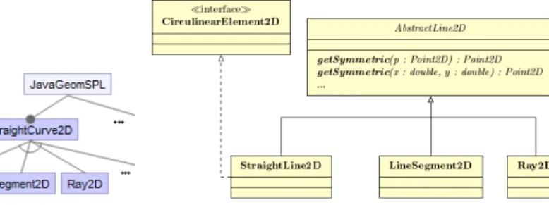
well identified features. Although not presented as an SPL, JavaGeom is a rel-evant and easily understandable case for demonstrating the applicability of our framework on the equivalent of a medium-size SPL. Let us consider the imple-mentation of a set of features as depicted in the FM on Fig. 1.StraightCurve2D
is a mandatory feature with three shown alternative features:Line2D,Segment2D, andRay2D. Focusing on the realization techniques (cf. Fig. 2), the abstract class
1
This notion is defined in Sec. 2 using a real feature-rich system. 2
Fig. 1: Features from JavaGeom Fig. 2: A detailed design excerpt of JavaGeom
AbstractLine2Dis a vp and its three variants, i.e.,StraightLine2D,LineSegment2D,
andRay2D, are created by generalizing/specializing its implementation. Features
from Fig. 1 seem to have a direct and perfect modular mapping in implemen-tation (cf. Fig. 2), e.g., «StraightCurve2Dimplemented by AbstractLine2D», or «Line2D implemented byStraightLine2D». But actually, this perfect modularity hardly exists.
Imperfect modularity comes from the fact that a feature is a domain concept
and its refinement in core-code assets is a set of vp-s and variants (even if they are modular), i.e., it does not have a direct and single mapping. For example, the featureLine2Duses several vp-s, such asAbstractLine2DandCirculinearElement2D
(other vp-s are not shown), the variant StraightLine2D (cf. Fig. 2), plus their technical vp-s (Sec. 3.2), as thegetSymmetric()vp of theAbstractLine2D. When a combined set of traditional techniques are used for implementing the variabil-ity, e.g., inheritance for StraightCurve2D, overloading for getSymmetric(), the
code is not shaped in terms of features. Therefore, the trace relation is n–to–m between the specified features to the vp-s and variants at the implementation. Moreover an SPL architect has to deal with a variety of vp-s and variants.
Our approach addresses the ability to trace this imperfectly modular vari-ability in implementation, which we define as follows: An imperfectly modular
variability in implementation occurs when some variability is implemented in a methodological way, with several implementation techniques used in combination, the code being not necessarily shaped in terms of features, but still structured with the variability traceability in mind.
3
A Three Step Traceability Approach
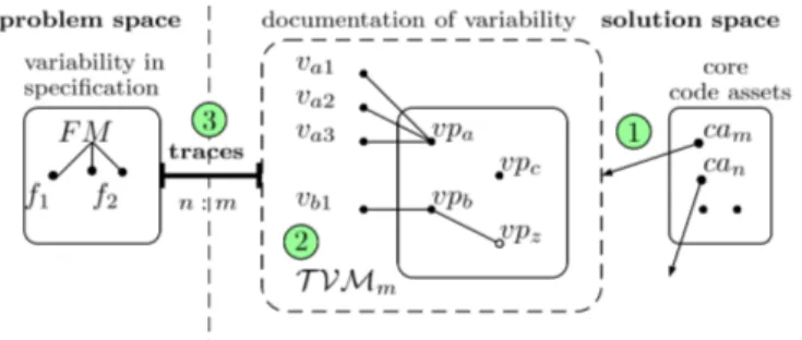
To trace imperfectly modular variability in implementation, we propose an ap-proach that follows three main steps (cf. Fig. 3):¬ capturing the implemented variability in terms of vp-s and variants, as abstract concepts, modeling (doc-umenting) the variability in terms of vp-s and variants, while keeping the con-sistency with their implementation in core-code assets, and ® establishing the trace links between the specified and implemented variabilities.
Fig. 3: Proposed traceability approach (T VMmstands for Technical Variability Model
( cf. Sec. 3.2) of the core-code asset cam, with vp-s {vpa, vpb, ...} and their respective
variants {va1, va2, ...}. While, {f1, f2, ...} are features in the FM.)
3.1 Capturing the Variability of Core-Code Assets (Step ¬)
The core-code assets that realize variability usually consist of a common part and a variable part. It can happen that a whole asset is also a variable asset. A core-code asset can be, e.g., a source file, package, class. The variable part consists of a mechanism (i.e., technique) for creating the variants, a way for resolving the variants, and the variants themselves. They are abstracted using the concepts of variation points (vp-s), variants, and their dependencies.
Let the set of all vp-s in an SPL be VP = {vpa, vpb, vpc, ...} for the set
of core-code assets, with variability or variable, CA = {cam, can, cao, ...}. We
assume that a vpx∈ VP is implemented by a single traditional technique tx∈ T .
The set T of possible techniques for vpxis then made explicit in our framework,
T = { Inheritance , Generic Type , Overriding , Strategy pattern , T e m p l a t e pattern , . . . }
A vp is not a by-product of an implementation technique [5], therefore we have to tag it in some way. "Tagging a vp" means to map the vpx ∈ VP concept to
its concrete varying element of any cax∈ CA. For example, we abstract/tag the
superclass AbstractLine2D (cf. Fig. 2) withvp_AbsLine2D, and its subclasses as variantsv_Line2D,v_Segment2D, andv_Ray2D, respectively. Depending on the size of variability and the used technique, the nature of a core asset element that represents a vp varies. We gathered their variety as characteristic properties of
vp-s. Their properties that are important to be captured are: granularity, relation
logic, binding time, evolution, and resolution.
Granularity. A vp in a core-code asset can represent a coarse-grained element
that is going to vary, e.g., a file, package, class, interface; a medium-grained element e.g., a method, a field inside a class; or a fine-grained element e.g., an expression, statement, or block of code.
Logic Relation (LG). The set of the logic relations between variants in a vp,
that are commonly faced in practice, is similar to the possible relations between features in an FM. Thus, a tx∈ T offers at least one of these logic relations,
Binding Time (BT ). Each vp is associated with a binding time, i.e., the
time when is decided for its variants, or when they are resolved. Based on the available taxonomies [6], the possible binding times for the vpxare:
BT = { Compilation , Assembly , Programming time , C o n f i g u r a t i o n , Deploy , StartUp , R u n t i m e }
Evolution (E V). Depending on whether a vp is meant to be evolved in the
future with new variants or not, it can beEV = {Open, Close}.
For example, thevp_AbsLine2Dhas a class level granularity (cf. Fig. 2). It is resolved at runtime to one of its alternative variants, v_Line2D, v_Segment2D, or
v_Ray2D, and we tag it as open as it is implemented as an abstract class. Another characteristic property of a vp is how it is resolved, i.e., whether a variant is added, removed or replaced by another variant. This matters during the process of product derivation, which is a possible usage of our framework.
3.2 Modeling the Implemented Variability (Step )
During this phase, the variability of a core-code asset caxis modeled in terms of
vp-s and variants as abstractions (cf. Fig. 3, step). We distinguish five types of vp-s that can be chosen from:
X = { vp , vp_unimpl . , vp_technical , vp_optional , vp_nested }
A resolution for each of them is given in Tbl. 1. The implementation technique
tx ∈ T of the vpx ∈ VP, which relation we write as (vpx, tx), describes three
main properties of the vpx: the relation logic for its variants, the evolution, and
the binding time. Possibly, other properties can also be abstracted and attached. Then, tx= {lgx, evx, btx, ...}, where lgx∈ LG, evx∈ EV, and btx∈ BT . So, when
the vpxis an ordinary vp (cf. Tbl. 1) we model the variability in a core-code asset
as a set of its variants V = {vx1, vx2, vx3, ...}, and the characteristic properties
derived from the vpx’s implementation technique tx. This leads to the following
definition:
vpx= {V, tx} = {{vx1, vx2, vx3, ...}, tx} (1)
As an illustration we present the ordinary vpx(cf. Tbl. 1) as in Fig. 4, numbered
with 1 . Similarly, a technical vp, e.g., the technical vpa of vpy, is represented as
in 2 . An optional vp is modeled as the vpzin 3 . We use the acronym opt here in
order to distinguish between the optional relations between variants in a vp and the optionality of the vp itself. Moreover a nested vp is illustrated as the nested
vpb of vpz, where the variant vz2 of vpz represents a common part for its three
variants {vb1, vb2, vb3}. Finally, the vpc = {{∅}, tc} in 4 is an unimplemented
vp. These types of vp-s can be combined, e.g., an optional vp can be ordinary,
unimplemented, or can have other nested or technical vp-s.
Instead of modeling the whole implemented variability at once and in one place, we model it in a fragmented way. A fragment can be any unit (i.e., a package, a file, or a class) that has its inner variability and that is worth to be separately modeled. For this reason, we designed specific models, named as
Table 1: Types of variation points that are commonly faced in practice
Types Description
Ordinary A vp is introduced and implemented ( i.e., its variants are realized) by a specific technique.
Unimplemented A vp is introduced but is without predefined variants ( i.e., its
vari-ants are unknown during the domain engineering).
Technical A vp is introduced and implemented only for supporting internally the implementation of another vp, which realizes some of the vari-ability at the specification level.
Optional The vp itself, not its variants, is optional ( i.e., when it is included or excluded in a product, so are its variants).
Nested vp When some variable part in a core-code asset becomes the common part for some other variants.
Technical Variability Models (T VM), which are created and maintained locally, i.e., closer to the core-code assets (cf. Fig. 3). They contain the abstractions of
vp-s and variantvp-s, their tagvp-s with core avp-svp-set elementvp-s, and devp-scribe the variability of a specific core-code asset. For example, the variability of a camwith six different
vp-s is modeled by the T VMmas in Fig. 4.
All the T VMs together constitute the Main Technical Variability Model (MT VM). Unlike the organization of features in an FM as a tree structure, in MT VM the vp-s reside in a forest-like structure. Moreover, the meaning of a vp is extended, i.e., it is the place at which the variation occurs [9], and represents the used technique to realize the variability.
(vpx, tx) vx1 vx2 vx3 1 (vpy, ty) vy1 (vpa, ta) va1 va2 2 (vpz, tz, opt) vz1 vz2≡ (vpb, tb) vb1 vb2 vb3 3 4 (vpc, tc) T VMm
Fig. 4: An example of the Technical Variability Model (T VMm) for a cam
3.3 Establishing the Trace Links (Step ®)
The last step of our approach (cf. Fig. 3, step ®) is to map the variability between the VM at specification level (i.e., features in an FM) and the MT VM at implementation level (i.e., vp-s and variants), by establishing the trace links between them.
Let us suppose that fx ∈ F M is a variable feature at specification level,
where F M = {f1, f2, f3, ...}. For mapping features to vp-s, we use a single
presents the variability realization trace link in implementation. When fx is
implemented ideally by a single variation point vpx, or conversely, we write:
fx 7−→ vpx, or implementedBy(fx, vpx). Similarly, fx can be implemented by a
single variant vxn ∈ V (cf. Sec. 3.2), i.e., fx 7−→ vxn. For example, the feature
StraightCurve2D (cf. Fig. 1) is implemented by vp_AbsLine2D (cf. Fig. 2), i.e.,
StraightCurve2D 7−→ vp_AbsLine2D, or Ray2D 7−→ v_Ray2D. When fx is
imple-mented by several vp-s, which can be from the same core-code asset or not, then
fx7−→ {vpx, vpy, vpz, ...}.
The mapping between features and vp-s is a partial mapping, as some fea-tures in F M are abstract feafea-tures (i.e., do not require an implementation), or they can be deferred to be implemented later.
4
Implementation and Application
We implemented the proposed framework as an internal DSL in Scala. The interoperability between Java and Scala enabled us to use the DSL in JavaGeom. To document and trace variability, the DSL provides two modulesfragmentand
traces, respectively. We used them to analyse 92% of the 35,456 lines of code from JavaGeom. The successful documentation phase resulted in 11 T VMs, all
of them being at the package level. We observed that vp-s in JavaGeom are implemented using up to three techniques, inheritance, overloading, and generic types. Then, we established the trace links between the specified features (cf. Fig. 1, which consist of 110 features extracted from its documentation) to the
vp-s and variants in implementation (cf. Fig. 2). We successfully traced 199 vp-s,
with 269 variants, showing the feasibility of our approach.
Capturing and documenting different types of vp-s and their implementation techniques during the variability traceability, as in JavaGeom, becomes impor-tant during the usage of trace links. For example, the relation logic between the variants in a vp is needed to check the consistency between the variability at the specification and implementation level. Similarly, knowledge of the binding time of vp-s is necessary during the product derivation.
5
Conclusion
Tracing the variability between the specification and implementation levels is an important part of the development process in SPL engineering. At the implemen-tation level, a combination of traditional variability implemenimplemen-tation techniques are actually used in many realistic SPLs, thus leading to a form of imperfectly
modular variability in implementation. The key contribution of our approach is
a three-step framework for capturing, documenting, and tracing this imperfectly modular variability, together with some DSL-based tool support.
A limitation of the DSL, but not of the framework itself, is that we could not apply it for tracing the variability at the finest granularity level, e.g., at the expression level, as our internal DSL in Scala uses reflection for tagging the vari-ability. Although using reflection is not mandatory, this helps to keep the strong
consistency between the abstractions of vp-s and variants with the core-code assets themselves. Although we used the DSL successfully in a real feature-rich system, we plan to extend this framework in supporting the documentation of the dependencies between the vp-s themselves and to integrate the DSL with an-other DSL that models the variability specifically at the specification level, such as FAMILIAR [1]. With these two extensions, we plan to apply our variability traceability framework to (semi)automated consistency checking of variability between the specification and implementation levels on several case studies.
References
1. Acher, M., Collet, P., Lahire, P., France, R.B.: FAMILIAR: a domain-specific lan-guage for large scale management of feature models. Science of Computer Pro-gramming (SCP) 78(6), 657–681 (2013)
2. Anquetil, N., Kulesza, U., Mitschke, R., Moreira, A., Royer, J.C., Rummler, A., Sousa, A.: A model-driven traceability framework for software product lines. Soft-ware & Systems Modeling 9(4), 427–451 (2010)
3. Becker, M.: Towards a general model of variability in product families. In: Work-shop on Software Variability Management. Editors Jilles van Gurp and Jan Bosch. Groningen, The Netherlands. http://www. cs. rug. nl/Research/SE/svm/proceed-ingsSVM2003Groningen. pdf. pp. 19–27 (2003)
4. Berg, K., Bishop, J., Muthig, D.: Tracing software product line variability: from problem to solution space. In: Proceedings of the 2005 annual research conference of the South African institute of computer scientists and information technologists on IT research in developing countries. pp. 182–191. South African Institute for Computer Scientists and Information Technologists (2005)
5. Bosch, J., Florijn, G., Greefhorst, D., Kuusela, J., Obbink, J.H., Pohl, K.: Vari-ability issues in software product lines. In: Software Product-Family Engineering, pp. 13–21. Springer (2001)
6. Capilla, R., Bosch, J., Kang, K.C.: Systems and Software Variability Management. Springer (2013)
7. Cleland-Huang, J., Gotel, O., Zisman, A.: Software and systems traceability, vol. 2. Springer (2012)
8. Coplien, J.O.: Multi-paradigm Design for C+. Addison-Wesley (1999)
9. Jacobson, I., Griss, M., Jonsson, P.: Software reuse: architecture, process and orga-nization for business success. ACM Press/Addison-Wesley Publishing Co. (1997) 10. Kang, K.C., Kim, S., Lee, J., Kim, K., Shin, E., Huh, M.: FORM: a feature-oriented
reuse method with domain-specific reference architectures. Annals of Software En-gineering 5(1), 143–168 (1998)
11. Kästner, C., Ostermann, K., Erdweg, S.: A variability-aware module system. In: ACM SIGPLAN Notices. vol. 47, pp. 773–792. ACM (2012)
12. Kim, J., Kang, S., Lee, J.: A comparison of software product line traceability ap-proaches from end-to-end traceability perspectives. International Journal of Soft-ware Engineering and Knowledge Engineering 24(04), 677–714 (2014)
13. Pohl, K., Böckle, G., van der Linden, F.J.: Software product line engineering: foundations, principles and techniques. Springer Science & Business Media (2005) 14. Schmid, K., John, I.: A customizable approach to full lifecycle variability