Acquisition and modeling of material appearance

Acquisition and Modeling of Material Appearance

by

Wai Kit Addy Ngan

B.S.E., Princeton University (2001)

S.M., Massachusetts Institute of Technology (2003)

Submitted to the Department of Electrical Engineering and Computer

Science

in partial fulfillment of the requirements for the degree of

Doctor of Philosophy

at the

Massachusetts Institute of Technology

August 2006

@

Massachusetts Institute of Technology 2006. All rights reserved.

A uthor ...

...

Department f Electical Engineering and Computer Science

t 30, 2006

Certified by...

...

...

Fr6do Durand

Associate Professor

Thesis Supervisor

Accepted by....

Arthur C. Smith

Chairman, Department Committee on Graduate Students

ARCH? VS

JAN

112007

LIBRARIES

Acquisition and Modeling of Material Appearance

by

Wai Kit Addy Ngan

Submitted to the Department of Electrical Engineering and Computer Science on August 30, 2006, in partial fulfillment of the

requirements for the degree of Doctor of Philosophy

Abstract

In computer graphics, the realistic rendering of synthetic scenes requires a precise descrip-tion of surface geometry, lighting, and material appearance. While 3D geometry scanning and modeling have advanced significantly in recent years, measurement and modeling of accurate material appearance have remained critical challenges. Analytical models are the main tools to describe material appearance in most current applications. They provide compact and smooth approximations to real materials but lack the expressiveness to rep-resent complex materials. Data-driven approaches based on exhaustive measurements are fully general but the measurement process is difficult and the storage requirement is very high. In this thesis, we propose the use of hybrid representations that are more compact and easier to acquire than exhaustive measurement, while preserving much generality of a data-driven approach.

To represent complex bidirectional reflectance distribution functions (BRDFs), we present a new method to estimate a general microfacet distribution from measured data. We show that this representation is able to reproduce complex materials that are impossible to model with purely analytical models. We also propose a new method that significantly reduces measurement cost and time of the bidirectional texture function (BTF) through a statisti-cal characterization of texture appearance. Our reconstruction method combines naturally aligned images and alignment-insensitive statistics to produce visually plausible results. We demonstrate our acquisition system which is able to capture intricate materials like fabrics in less than ten minutes with commodity equipments.

In addition, we present a method to facilitate effective user design in the space of ma-terial appearance. We introduce a metric in the space of reflectance which corresponds roughly to perceptual measures. The main idea of our approach is to evaluate reflectance differences in terms of their induced rendered images, instead of the reflectance function itself defined in the angular domains. With rendered images, we show that even a simple computational metric can provide good perceptual spacing and enable intuitive navigation of the reflectance space.

Thesis Supervisor: Fr6do Durand Title: Associate Professor

Acknowledgments

First and foremost, I would like to thank my advisor Professor Fr6do Durand for his support and guidance for the past four years. His ever-flowing stream of insights and ideas in broad areas of computer graphics have never ceased to amaze me. Working with him has been a fruitful and enjoyable learning experience. I am also very grateful that he has made himself available to me most of the time despite his immense workload. In particular, my thesis would not have been completed in time if Fr6do had not presented the two papers at EGSR 2006 on my behalf. Our discussions also go beyond research - I have enjoyed chatting about photography and travel with him. Fr6do has played an important role in making my time in graduate school a pleasant experience.

I would like to thank Professor Leonard McMillan for advising me during my first year of graduate studies. I would also like to thank Wojciech Matusik for his collaborations on more than a few projects, including most work presented in this thesis as well as other ones. His devotion and relentless energy are contagious and have propelled me to try to think and work harder. I also would like to express my gratitude to Hanspeter Pfister, who co-advised me on several projects at MERL.

I would like to thank my thesis committee members Professors Jovan Popovic and Edward Adelson for their time and input on the thesis, especially given the tight schedules. I want to thank Eric Chan for his insightful inputs on both graphics research and photography, and being a great officemate. I would also like to thank Sara Su who has been a supportive officemate and practically proofread every paper I have written, including this thesis. Soonmin Bae, Jiawen Chen, Barb Cutler, Paul Green, Tilke Judd, Jan Kautz, Jaakko Lehtinen, Tom Mertens, Sylvain Paris, Marco da Silva, Daniel Vlasic, Robert Wang, Matthias Zwicker have all provided valuable feedbacks to my research. Tom Buehler has helped me to produce several paper videos, and Bryt Bradley has been the magical force behind the scenes of everything the graphics group has accomplished. I would like to thank all members of the MIT Computer Graphics Group for their support.

Finally, I would like to thank my family for their love and support over many years. My girl-friend Joyce has provided more than spiritual support -she has provided tremendous help in the construction of various hardware setups and measurement targets. Of course, I am even more grate-ful for her love, patience and support. This thesis is dedicated to her.

Contents

1 Introduction

1.1 C ontext . . . . 1.2 Modeling of Homogeneous Reflectance . ...

1.3 Measurement and Modeling of Spatially-Varying Reflectance .. 1.4 Material Appearance Model Navigation . ...

1.5 Thesis Overview ... 2 Background

2.1 Definitions and Notations ... 2.1.1 Radiometry ... 2.1.2 Reflectance ...

2.2 Comparison of Reflectance Representations . . 2.2.1 Limitations ... .... 2.3 Reflectance Measurement ... 2.3.1 BRDF Measurement ... 2.3.2 BTF Measurement ... 2.3.3 Reflectance Fields ... 2.4 BRDF Representations ... 2.4.1 Analytical Models ...

2.4.2 Generalized microfacet model ... 2.4.3 Data-driven Representations ... 2.5 Spatially-Varying Reflectance . . . . 2.5.1 Approximations ... 25 . . . . . 25 .. .. ... .. 25 .. .. .. .. . 26 . . . . . 30 .. .. .. .. . 31 . . . . . 3 1 .. .. ... . . 31 .. .. ... . . 34 .. .. ... . . 35 .. .. ... . . 36 .. .. .. ... 36 . . . . . 4 1 . . . . . 4 1 . . . . . 42 .. .. ... .. 42

2.5.2 BTF . . . 43

2.6 Statistical Analysis of Reflectance and Texture . ... 44

2.6.1 Texture Modeling and Synthesis ... . . . 44

2.6.2 Light- and View-Dependent Statistics . ... 45

2.7 Perceptual Study of Material Appearance . ... 46

2.7.1 Reflectance Perception under Unknown Illumination ... 46

2.7.2 Perceptual Distance in Reflectance Space . ... 47

3 Analysis of Isotropic BRDF Models 49 3.1 D ata Set . . . 50 3.2 Data Processing ... 50 3.3 M ethodology ... 51 3.3.1 BRDF models ... 51 3.3.2 Fitting BRDFs ... 52 3.3.3 Error M etric ... 52 3.4 Analysis ... . ... ... . 53

3.4.1 Fitting quality of the models . ... .. 53

3.4.2 M ultiple lobes ... 57

3.4.3 Evaluation of different microfacet distributions . ... 58

3.4.4 Fresnel effect ... 59

3.5 Formulation of the specular lobe ... .... 59

3.6 Summary .... ... ... 62

3.7 Discussion ... ... 63

4 Representing BRDFs with a Sampled Microfacet Distribution 65 4.1 Background ... 66

4.1.1 Microfacet Theory ... 66

4.1.2 Ashikhmin's Microfacet-based BRDF Generator . ... 67

4.2 Estimation of the Microfacet Distribution from Measured Data ... 69

4.3 Data Analysis ... 70

4.3.1 Measurement of anisotropic materials . ... 70 8

4.3.2 Analytical Models ... . . 4.3.3 Generalized Microfacet Model ... 4.4 Reconstruction ...

4.5 Application to Isotropic BRDFs . . . . 4.5.1 Results .. ... ... ... 4.6 Summary ...

4.7 Discussion ...

5 Statistical Acquisition of Texture Appearance 5.1 Acquisition ... 5.1.1 Implementation ... 5.1.2 Alternative Setup ... 5.2 Reconstruction ... 5.2.1 Histogram Statistics ... 5.2.2 Data Preprocess ... 5.2.3 Texture Generation ... 5.2.4 Texture Tiling ... 5.3 Hardware Implementation . . . . 5.3.1 Data Preparation ... 5.3.2 Real-time Rendering ... 5.4 Results ... . ...

5.4.1 Acquisition and reconstruction ... 5.4.2 Validation ... 5.4.3 Statistical characterization . . . . 5.4.4 Sampling Density ... 5.5 Limitations ... 5.6 Summary ... 5.7 Discussion ...

6 Image-based Navigation of Analytical BRDF Models 6.1 Related Work ... 9 81 . .. ... .. .. 82 . .. ... .. .. 82 . .. ... .. .. 84 . .. ... .. .. 84 . .. .. ... .. 85 . .. .. ... .. 87 . .. .. ... .. 88 . .. ... .. .. 90 . . . . . 91 . .. .. .. ... 9 1 . .. .. .. ... 92 . .. .. .. ... 92 . . . . . 92 . .. .. .. ... 94 . . . . . 96 . .. .. .. ... 98 . .. ... . ... 99 . .. .. .. ...101 . .. ... .. ..103 105 106

6.2 BRDF Metric ...

6.2.1 Image-driven Metric ... 6.2.2 Metric Evaluation ... 6.3 Fast Distance Computation ...

6.3.1 Embedding in a Unified Euclidean Space 6.4 Navigation Interface ...

6.4.1 Image Pre-rendering ... 6.4.2 Interface Implementation ... 6.5 Navigating Across Different Models ... 6.6 Summary ... 6.7 Discussion ... . . . 108 . ... .. .. ... .. .108 . ... .. .. ... .. .109 . ... .. ... .. .. .114 . . . .114 .. .. .. ... .. .. .115 .. .. .. ... .. .. .116 . . . 117 . . . .119 ... 121 ... 121

7 Conclusions and Future Work 7.1 Conclusions ... ... 7.2 Analytical and Data-Driven Representations ... 7.3 Future Work ... ... 125 . . . 125

. . .. . . . 127

List of Figures

2-1 Geometry of surface reflection ... 27 2-2 Image-based measurement of isotropic BRDFs [66, 68]. The surface

nor-mals of the spherical sample provide two degrees of freedom, the rotating light provides the third for the 3D isotropic BRDF . ... 32 2-3 Our acquisition setup for anisotropic materials. The cylinder tilt, surface

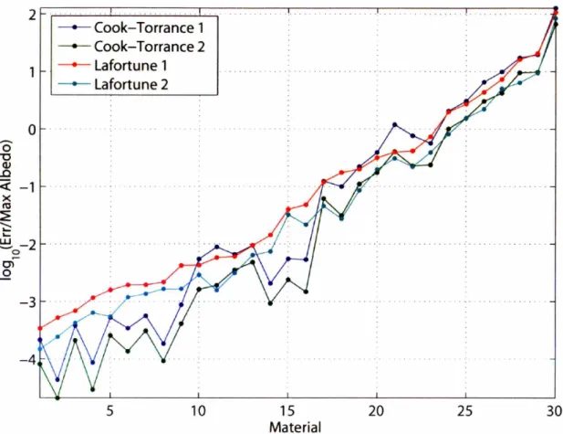
normal variation, light position and strip orientation each contributes to one degree of freedom for acquiring the 4D BRDF . ... 33 3-1 The normalized fitting errors (logarithmic scale) of five analytic models to

our isotropic data set of 100 BRDFs. The BRDFs are sorted by the errors in the Lafortune model (Red) for the purpose of visualization. ... 55 3-2 Fitting the measured "green-metallic-paint" BRDF with the seven models.

Clockwise from upper left: Measured, Ward, Ward-Duer, Blinn-Phong, He, Ashikhmin-Shirley, Cook-Torrance, Lafortune. . ... 56 3-3 Polar plots of the measured "green-metallic-paint" in the incidence plane

compared to the fits from the Ward, Cook-Torrance and Lafortune models. Cubic root applied. ... ... 57 3-4 The fitting errors (logarithmic scale) with one/two lobes of the Cook-Torrance

and the Lafortune models. ... 58 3-5 Fitting the measured BRDF "nickel" with the multi-lobe Cook-Torrance

and Lafortune models. Left to Right: Input, Torrance 1 lobe, Cook-Torrance 2 lobes, Lafortune 1 lobe, Lafortune 2 lobes. ... 59

3-6 The V -R lobe compared with the H -N lobe remapped to the outgoing

directions ... 60

3-7 Side and top-down view of the measured "PVC" BRDF, at 550 incidence. (Cubic root is applied to the BRDF for visualization.) Its specular lobe exhibits a similar asymmetry to the H -N lobe. . ... 61

4-1 Target cylinder covered with velvet. . ... .. 71

4-2 Sampling density for a typical measured BRDF at a particular view direc-tion (0 = 45, 0 = 0). Blue: data bins containing valid measurements. .... 72

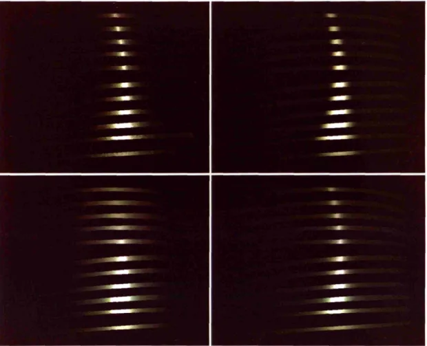
4-3 Brushed Aluminum: One measurement photograph (upper left), recon-struction using Ward model (ax = 0.04, ay = 0.135) (upper right), recon-struction using Poulin-Fournier model (n = 3000, d = 0.18, h = 0.5)(lower left), reconstruction using Ashikhmin model with sampled microfacet dis-tribution (lower right) ... ... 73

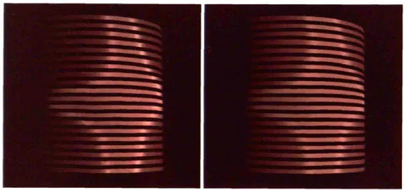
4-4 Left: Purple satin -one input photograph. Right: -reconstruction using sampled microfacet distribution. . ... .... 74

4-5 Left: Brushed aluminium macro photograph. Right: deduced microfacet distribution (log plot). ... 74

4-6 Left: Purple satin macro photograph with sketched double cones. Right: deduced microfacet distribution (log spherical plot). . ... 75

4-7 Left: Red velvet macro photograph. Right: deduced microfacet distribution (log spherical plot) . ... ... 75

4-8 Full reconstruction of purple satin (left) and yellow satin (right). ... 76

4-9 Estimated microfacet distribution of the measured BRDF nickel. ... 77

4-10 Comparing the microfacet distribution approximation (right) to the mea-sured BRDF nickel (left) ... 78

5-1 Acquisition setup for spatially-varying materials. . ... 83

5-2 Reconstruction pipeline. ... 85

5-4 View interpolation/extrapolation in spherical coordinates. The view direc-tions are grouped into classes with similar incidence angle 0 and form rings on the hemisphere. With this semi-uniform structure, the view direction can be interpolated or extrapolated in a bilinear fashion. . ... 88 5-5 Rendered images of the measured materials. . ... 93 5-6 Validation with materials from the Bonn BTF database. ... . . 95 5-7 Comparing approximations to the measured materials knitwear- 1 and

green-knitwear ... ... 96 5-8 Texture reconstruction at o) = (60,0). Row 1: Carpet from Koudelka et al.

[51], Row 2: Measured material carpet-i. . ... . . . . 97

5-9 Comparing the interpolated pixel histograms to the Bonn measurement of the material proposte ... 97 5-10 Comparing different sampling density (Proposte). . ... . 98 5-11 Reconstruction of wool at different sampling densities, compared to the full

resolution data (81 views x 81 lights) from Bonn BTF Database. ... 99 5-12 Reconstruction of the impalla material at different sampling densities,

com-pared to the full resolution data (81 views x 81 lights) from Bonn BTF Database. ... 100 5-13 Comparing our reconstruction technique against direct interpolation at low

sampling densities (Wool BTF). ... 100 5-14 Failure case for the Lego BTF [o• = (60, 0)]. Our reconstruction is unable

to reproduce the disparity, but the shadow elongation is partially captured. . 101 5-15 Failure case for the Lego BTF: original vs our reconstruction. ... 102 5-16 Indoor scene rendered using 4 textures acquired and reconstructed with our

technique . . ... . ... ... . 103 6-1 Photoshop's Variations interface ... . . . ... . 107 6-2 The Ward model, varying along the roughness dimension (a = 0.01 to

0.37). Row 1: uniformly spaced according to the BRDF space L2 metric, Row 2: uniformly spaced according to our image metric. ... 108

6-3 Comparing the gloss ratings reported by human subjects and the 10-steps cumulative distances reported by our image-driven metric (Blue), and the direct L2 metric with LAB (Green) and RGB (Red). The linear fit proposed by Pellacini et al. is also shown (Black). d is the distinctness-of-image parameter defined as d = 1 - a, where a is the roughness parameter in the

original Ward model. Adapted from [85] with author's permission. ... 110 6-4 The Lafortune model, varying along cz = 0.54 to 0.58, exponent n = 800.

Row 1: linearly spaced along cz, Row 2: uniformly spaced according to our image-driven metric. ... 111 6-5 Plot of distances from the Ward BRDF at a = 0.07 to 25 samples ranging

from a = 0.01 to 0.36. We compute our image-based metric with ren-derings using three different environment maps and compare to the BRDF-space L2 metric. The distances from the different metrics are brought to the same scale by minimizing the least-square errors over all (25 x 24) pairwise distances. ... 113 6-6 Screenshot of the navigation interface. The current model is the

Cook-Torrance model, and the user is at the roughness/grazing tab. The center image is the current BRDF, and the surrounding ones are the four equidis-tant neighbors. ... 116 6-7 Equidistant neighbors (small red circles) are found by walking along the

isoparameter lines (dashed lines). The neighbor at the desired distance is found when the segment intersect the circle (sphere). The orange lines highlight the grid samples that are queried during the search. The black lines indicate other grid samples. . ... ... 118 6-8 Illustration of the manifolds spanned by two analytical BRDF models in an

abstract unified BRDF space. Point on the black curves represent instance of two BRDF models. Given a current BRDF, we want to find BRDFs on an alternative model that are close but cannot be represented by the current analytical model. We wish to propose materials such as B' because its distance dyl to the current model is large. See text for detail ... 120

6-9 The conversion tab showing the neighbors in the union space of all models. Note that all the neighbors show some effects which are not expressible with the current model (Blinn-Phong). ... . 123

Chapter 1

Introduction

Recent advances in computer graphics have enabled the production of highly realistic ren-dered images when a precise description of a scene is provided. A complete scene de-scription includes surface geometry, lighting, and material appearance. While 3D geome-try scanning and modeling have advanced significantly in recent years, measurement and modeling of accurate material appearance have remained critical challenges. Analytical reflectance models are the main tools used to describe appearance in most current appli-cations. They provide compact and smooth approximations to real materials but lack the expressiveness to represent complex materials. In the production industry, the realism of materials in graphics renderings has improved tangibly, but the improvement is not en-tirely the result of advancement in appearance techniques. To some extent, increase in raw computation power has provided improved image quality with existing models. More importantly, graphics artists have become more experienced in exploiting existing tech-niques creatively. However, several classes of materials remain difficult to reproduce, most notably human skin and fabrics. Direct exhaustive measurement of real materials is a vi-able alternative for materials that are difficult to model (e.g. [10]), but its use is far from widespread due to the high cost of measurement time and equipment setup. In this thesis, we propose the use of hybrid representations that are more compact and easier to acquire than exhaustive measurement, while preserving much generality of data-driven approaches.

1.1 Context

In the early days of computer graphics, simple empirical models were developed to approx-imate local reflection. Models like Lambert's and Phong's provide only crude qualitative approximations to material appearance. Over the past few decades, numerous models have been proposed for improved fidelity, flexibility and computation efficiency. However, there has been a lack of studies to compare these models quantitatively. The first contribution of this thesis is to provide such a study. We quantitatively validate a number of reflectance models based on high quality measured data. In the process, we gain important insights into the merits of different model formulations. In addition, our new measurements of anisotropic materials show that existing analytical models lack expressiveness needed to handle complex appearance. A semi-parametric representation, based on general micro-facet distributions [1], is able to provide much better approximations to the measurement while still achieving good compactness compared to full-blown data. We demonstrate an efficient method to fit measured data to this representation.

Direct acquisition of material appearance has become very popular over the past decade for several reasons. As light transport algorithms mature, they have become more sensitive to the quality of the input data. Measured data are either used to fit analytical models or are directly used for rendering. If the measurement resolution is high enough, direct rendering can provide the highest quality since it is not bounded by the expressiveness of any particular model. Moreover, the increase in computation power and storage has made measurement and processing of reflectance data, often in size of gigabytes, more tractable. Also, the image-based approaches introduced recently (e.g. [65]) allow for more efficient measurement by collecting many reflectance samples in a single image. However, quantities such as spatially-varying reflectance are still unwieldy to acquire due to the high dimensionality. State-of-the-art measurement devices require expensive robotics setup, and the measurement process is very time-consuming. In this thesis, we propose a method to reduce acquisition cost and time significantly. The main idea of our approach is to measure visually important statistics which are insensitive to precise registration. By removing the requirement of precise alignment, the measurement setup can be much simplified: no

robotics setup is required, and multiple views can be acquired in a single image. Such dramatic reduction in measurement precision and sampling does come at a cost: materials with strong parallax or sharp specularities are not reproduced faithfully. Nonetheless, we will show that our technique is general enough for a large class of materials and degrades gracefully for the failure cases.

Another important element of the appearance reproduction pipeline is user design. In most current graphics applications (e.g. movies, games), material appearance is typically specified with analytical models rather than measured data. Choosing the right parameters for a particular model, however, is often difficult because these parameters can be non-intuitive for users and can have non-uniform effects on the rendered image. Ideally, a given step in the control parameter space should produce a predictable and perceptually-uniform change of the rendered image. To alleviate this issue, software developers often include ad-hoc remapping of the parameters. However, a more systematic solution is desirable in order to make material modeling more intuitive. Systems that employ psychophysics have produced important advances in this direction [85], but the main drawback of these systems is the requirement of extensive user studies, which limits their scalability. In this thesis, we introduce a metric in the space of material appearance which corresponds roughly to perceptual measures. The main idea of our approach is to evaluate appearance differences in terms of the rendered images, instead of the radiometric quantity itself defined in the angular domains. With rendered images, we show that even a simple computational metric can provide good perceptual spacing and enable more intuitive navigation of the appearance space.

To sum up, the work presented in this thesis tackles a number of issues in differ-ent stages of the material appearance reproduction pipeline. For acquisition, our work on statistical reconstruction of texture appearance allows efficient measurement of high-dimensional reflectance data. For modeling, we validate existing models with measured data and provide guidance for their use. In addition, we demonstrate the limited expres-siveness of pure analytical models and show that a semi-parametric model is needed for approximating complex materials. Finally, for user design, we introduce a image-based metric that corresponds to perceptual measures and facilitates an effective navigation

in-terface. In the following sections, we will introduce each component of the thesis in more details.

1.2 Modeling of Homogeneous Reflectance

The Bidirectional Reflectance Distribution Function (BRDF) describes how light interacts at a surface point. It is a function of the incoming and outgoing directions that describes how much of the incoming light is reflected. The BRDF can fully describe the appear-ance of homogeneous materials, e.g. most plastic and smooth metals. Early models such as Phong [87] and Lambertian [54] were not introduced formally as BRDF models, but they govern the same relationship. BRDF models can be divided roughly into two classes: empirical models seek to emulate the characteristics of material reflection qualitatively [6, 118, 52], while physically-based models derive the quantities from first principles of physics[ 13, 42]. While the latter models are physically plausible, they should not be im-mediately considered as true models as they all make significant simplifying assumptions. While new BRDF models are often introduced together with a few measured materials to illustrate their capabilities, no quantitative comparisons between different models have been published. We believe the main reason for the lack of validation is the difficulty of obtaining high-resolution measurement. In 2003, Matusik et al.[68] published a data set of over a hundred BRDFs measured at high dynamic range and high angular resolution. With the presence of such a data set, we have the opportunity to provide a detailed quantitative comparison between a number of popular models. To the best of our knowledge, this is first time multiple BRDF models are validated and compared using a large measured data set. The detailed validation results will be presented in Chapter 3.

An interesting alternative to pure analytical BRDF models was introduced by Ashikhmin et al.[1]. In their microfacet-based BRDF generator, a physically plausible BRDF can be created from an arbitrary distribution of microfacets. We derive a simple method to invert the process and estimate a discretely sampled microfacet distribution from BRDF mea-surements. Given the much higher degrees of freedom in this BRDF representation, it is not surprising that this representation provides higher fidelity than pure analytical models.

Since Matusik et al.'s data set is limited to isotropic materials, we have extended their mea-surement setup and measured a few anisotropic materials. We show that for some complex anisotropic materials, the sampled microfacet distribution is the only method that can qual-itatively resembles the true BRDF. Our inversion procedure and the associated results will be presented in Chapter 4.

1.3 Measurement and Modeling of Spatially-Varying

Re-flectance

The most common solution to model spatially-varying appearance is the use of texture map-ping. Texture mapping typically maps each surface location to a color value and is suitable for cases where the spatial variation is solely due to color differences. While a BRDF can be coupled with the texture by multiplication, intricate effects due to meso-scale geom-etry is not reproduced. A number of techniques have been proposed to augment texture mapping. Bump mapping simulates the effect of surface roughness by perturbing surface normals [7]. Horizon mapping enhances bump mapping by handling self shadowing effects [72, 105]. In both cases, an auxiliary map has to be provided by the user through estimation. A more general representation for spatially-varying reflectance is the Bidirectional Texture Function (BTF) [23], a 6D function that depends on the incoming and outgoing directions, as well as spatial locations. Current BTF measurements all require precisely calibrated equipments, as well as robotics setup for positioning the light, camera and the texture patch itself. Due to the large size of the BTF representation, most recent research has focused on data compression. In this thesis, we instead focus on an alternative representation that allows significant reduction in terms of measurement cost and time. Our representation is a hybrid representation that combines images with perfect correspondence and aggregate statistics that are alignment-insensitive. By removing part of the required correspondence in a traditional BTF measurement, we are able to measure BTF appearance through a much simplified setup. Complex materials like fabrics can be captured in less than ten minutes without elaborate calibration, and their appearance are reproduced in a visually plausible

way. In Chapter 5, we will describe the acquisition setup and our reconstruction procedure, followed by results and discussions.

1.4 Material Appearance Model Navigation

Although measurement of real materials has become popular in recent years, in most graph-ics applications, material appearance is still dominantly specified with analytical models. Despite the fact that many models have been introduced since Phong, in many commercial applications, only the simplest models are employed. The reason is twofold. First, many models are complex mathematically, and it is difficult for users to have an intuitive under-standing. Second, the parameters of the models are often quantities that do not necessarily map to appearance changes uniformly. Using data from human experiments, Pellacini et al.[85] redefine and rescale the parameter axes of the Ward model [118] in a perceptually uniform way. However, the requirement of human experiments on such an approach limits its scalability to more complex models. In this thesis, we introduce a computation metric that roughly corresponds to perceptual spacing in the space of reflectance. The main idea of our approach is to evaluate reflectance differences in image space: instead of comparing reflectance in its native angular domain, we compare them in terms of their induced ren-dered images. We show that even a simple metric in the image space can produce visually plausible spacing. However, while we believe that an image-driven metric is a step in the right direction, we do not claim it to be a perceptual metric as it has not been validated by psychophysical experiments. In Chapter 6, we will explain the metric in details. We will also demonstrate a user interface based on this metric and show that it offers intuitive and uniform navigation in the space of analytical reflectance models.

1.5 Thesis Overview

In Chapter 2, we introduce the fundamental concepts and terminology in the field of ma-terial appearance and provide a broad overview of previous research in measurement and modeling. In Chapter 3, we present our quantitative validation of homogeneous reflectance.

In Chapter 4, we describe our method to estimate a generalized microfacet distribution from measured data and demonstrate its effectiveness on complex anisotropic materials. In Chapter 5, we present our work in statistical acquisition and reconstruction of spatially-varying reflectance. In Chapter 6, we describe our image-driven reflectance metric, and a visual interface based on the metric that allows intuitive navigation of appearance models. Finally, we conclude the thesis and provide directions for future work in Chapter 7.

Chapter 2

Background

The study of material appearance is an important subject in computer graphics, as well as physics, computer vision and perceptual science. In computer graphics, accurate reproduc-tion of material appearance is a crucial element in realistic rendering. The study of mate-rial appearance can be roughly categorized into measurement, representation, modeling and rendering. To make our discussion more concrete, we will first introduce the common nota-tions and defininota-tions in radiometry, as well as important reflectance representanota-tions such as the Bidirectional Reflectance Distribution Function (BRDF) and the Bidirectional Texture Function (BTF). We will then provide a comparison of these different representations and discuss their limitations. Next, we will review the different measurement techniques in pre-vious research. We will then discuss prepre-vious work on statistical studies of reflectance and texture. In the final section, we will briefly describe previous work on human perception of materials and their implications on graphics techniques.

2.1 Definitions and Notations

2.1.1

Radiometry

Radiometry is the field that studies the measurement of electromagnetic radiation. In com-puter graphics, light transport is mostly simulated at the geometric optics level. Wave phenomena like diffraction and interference are typically ignored (Exceptions include [76,

3, 106]). In this thesis, we also ignore effects of polarization, fluorescence, and phospho-rescence.

Radiant Power or Flux

Flux, often denoted as D, expresses the amount of energy per unit time. Total emission from light sources is often described in terms of flux. The unit of flux is Watt [W].

Irradiance

Irradiance (E) is defined as flux per unit surface area and is often used to describe the amount of energy striking the surface from a certain direction. The unit of irradiance is Watt per meter squared. [Wm- 2_]

de

E = (2.1)

dA

Radiance

Radiance is the most fundamental quantity in radiometry. Radiance is measured in flux per unit projected area per unit solid angle. Solid angle is measured in steradians and represent the subtended surface area when the region is projected to the unit sphere. One favorable property of radiance is that it remains constant along a ray through empty space. This makes it a convenient quantity to propagate in raytracing algorithms. The unit of radiance is Watt per steradian per meter squared. [Wsr-Im- 2]

d2_ d24

L d

d

(2.2)

2.1.2 Reflectance

The following descriptions of the reflectance quantities mostly follow the convention of Nicodemus et al. [81]. Similar descriptions can be found in [33, 86].

dw

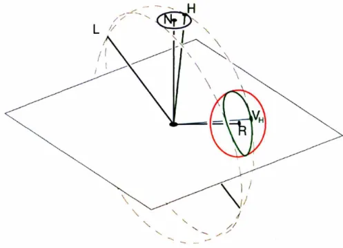
Figure 2-1: Geometry of surface reflection Bidirectional Scattering-Surface Reflectance-Distribution Function

The bidirectional scattering-surface reflectance-distribution function (BSSRDF) describes the relationship between incoming irradiance and outgoing radiance on a general surface. In Figure 2-1 we show a surface patch approximated by a plane. Let the incident radiance from direction (0i,

4i),

transport is unspecified, dLr and dr,. should be linearly related due to the linear nature of reflections. We have:

dLr = S -d Di = S -Li -cos Oi -doi -dA (2.3) The factor S depends on the location of incoming and outgoing locations, as well as the directions of the incoming and outgoing rays. Thus, S is a 8-dimensional quantity:

This quantity S is called the bidirectional scattering-surface reflectance-distribution function (BSSRDF). Its unit is per steradian per meter squared [sr-lm-2]. Given S and

a complete description of incoming radiance from all directions, we can compute the out-going radiance on every point of the surface by integrating Equation 2.3 over the incident locations and incident directions.

The BSSRDF is a very general property of a surface and captures all kinds of light transport, including subsurface scattering, in a black-box manner. However, the high di-mensionality of the BSSRDF makes it very difficult to measure and use. As a result, it is often reduced to simpler representations by imposing certain assumptions or restrictions. We will now discuss two of these cases.

Bidirectional Reflectance Distribution Function

If we assume that the material is uniform, the BSSRDF S and the differential outgoing radiance dLr should both be independent of (xr,Yr). Without loss of generality, we can set (xr,yr) equal to (0, 0). Now, we assume the entire surface is irradiated by radiance Li(0i, Oi), from direction (0i, 4i) over the solid angle element dooi. We can integrate Equation 2.3 over the incident locations:

dLr(0i, i; 0r, r, 0, ) =

j

(2.5)

Nicodemus et al. [81] define the bidirectional reflectance distribution function (BRDF) as:

PI (i, Oi; Or, Or) = f S(Oi, Xi, x,i; Or, r, 0)dAi (2.6)

In this formulation, the BRDF sums up all the scattering contribution over the entire area. Substituting into Equation 2.5, we have:

Pl(Oi,•i;Orr) = dLr(Oi, i; Or,r,0,0) (2.7)

Intuitively, the BRDF relates the outgoing radiance at a particular location to the in-coming irradiance on a nearby flat surface patch. Given the inin-coming irradiance over the full hemisphere, the BRDF fully specifies the outgoing radiance in all directions.

However, the BRDF is commonly defined in a different way. Since the intensity of scattered rays falls off very quickly for many materials, one way to simplify the BSSRDF is to completely ignore contributions from the neighborhood. In this case, the BRDF can be seen as a slice of the BSSRDF:

p2(Oi, hOi' Or, Or) = S(Oi, Oi, 0, 0; Or, r; 0,0 ) (2.8) While the second definition is more commonly assumed, we should note that with most measurement devices, the measured BRDFs correspond more closely to the first definition. This is because, in most measurement devices, the entire sample is lit by the light source. To accurately measure a BSSRDF slice, we would need the ability to illuminate a narrow area of the sample (e.g. using a laser beam).

Bidirectional Texture Function

Dana et al. [23, 24] introduced the term bidirectional texture function (BTF) to represent

spatially-varying reflectance. It is a 6D quantity R(Oi,0i;Oo,0 0 ,x,y). Again it can be

de-fined either as the BSSRDF integrated over the incident locations, or simply a slice of the BSSRDF:

R1

(Oi,i;

j

R2(Oi, i; Or, r, X,y) = S(Oi, Ci,xi = x, yi = y; 00o, 0 ,x0 = x, yo = y) (2.10)

With the BTF, nonlocal subsurface scattering effects are ignored or pre-integrated. It encodes all other effects such as shadowing, masking and multiple scattering.

2.2

Comparison of Reflectance Representations

Among the different representations of reflectance described in the previous section, it is natural to ask which one to use when we want to model the appearance of a particular surface. The representations can be ordered in an ascending order of complexity: BRDF, BTF, BSSRDF. In addition, at a even higher complexity, we can model the surface with the actual micro-geometry at a fine resolution. Assuming we have an ideal light transport simulator, the micro-geometry representation can be readily converted to the BSSRDF or its derived quantities. For example, Westin et al. [119] use Monte Carlo techniques to approximate BRDFs from micro-geometry. Becker and Max [5] describe a method to convert between displacement map, bump map, and BRDF such that transition between the three representations is smooth when they are used at the same time.

If we assume that the explicit micro-geometry of a surface is available through mod-eling or measurement, it may seem reasonable to always use this representation directly. However, there are a number of reasons that this is often not a good solution. First, if the scale of geometric variations is small enough with respect to our rendering resolution, using the full micro-geometry is simply overkill. In addition, we would need to pay spe-cial attention to avoid aliasing due to undersampling. Second, the perfect conversion from micro-geometry to BSSRDF is only possible with a ideal light transport simulator, which would need to simulate all kinds of physical phenomena present. In practice, the conversion is only an approximation. On the contrary, by measuring the less complex representations such as BRDF or BTF directly, all the physical interactions can be treated in a black-box manner. In a setting where rendering time is limited (e.g. 3D games), it is typically imprac-tical to simulate global illumination effects. In these cases, BRDF and BTF can provide realism that is otherwise not achievable, since the material level scattering is pre-integrated. Finally, it is a strong assumption that we can obtain the micro-geometry of real materials as the three-dimensional measurement at that scale is generally difficult.

2.2.1 Limitations

When employing the various reflectance quantities, it is important to understand their limi-tations. First of all, the BSSRDF and its derived quantities are all defined on a flat geometry and do not provide accurate silhouettes. This is particularly visible when the BTF is applied due to the abrupt transition at the silhouettes.

The second limitation is concerned with surface curvature. Since the BRDF is defined at a confined location, it does not depend on the curvature of the surface. However, BSS-RDF and BTF are typically defined and measured on flat surfaces. When these quantities are applied to a parameterized surface with non-zero curvature, the reflectance can change in a non-trivial manner. However, the curvature assumption is seldom mentioned in the literature, and BTFs are often applied to surfaces without such considerations. Notable exceptions are the works by Wang et al. [116] and Heidrich et al. [44]. In the former work, the view-dependent displacement map is pre-computed for various surface curvatures. In the latter case, global illumination effects are precomputed for height fields on a flat geom-etry and changes due to surface curvature are approximated when the height field is applied to curved surfaces.

2.3 Reflectance Measurement

2.3.1 BRDF Measurement

Traditionally, the BRDF is measured using gonio-reflectometers [82, 14]. A gonio-reflectometer consists of a light source and a detector, both of which can be positioned at any specified directions by motors or robotic arms. A flat sample of the measured material is placed in the center. Individual BRDF samples can be measured by positioning the light source and the detector from the desired directions. Since the detector is only responsible for measur-ing one sample at a time, sophisticated spectro-radiometer with high dynamic range and high spectral resolution can be employed. However, since only one value is recorded at a time, it is very time-consuming to capture a 3D or 4D BRDE As a result, it is impractical to use a gonio-reflectometer to measure BRDFs at high angular resolution.

Ward [118] accelerates the BRDF measurement process by measuring multiple samples at the same time. He uses a hemispherical half-silvered mirror with a flat sample in the center. The outgoing radiance from the flat sample to all directions can be observed at the same time, using a CCD camera with a fish-eye lens. With this setup, the measurement time is much reduced since only the light direction needs to be varied. However, quality from this setup is relatively low due to the multiple optical elements, and angular resolution near grazing angle is limited. More recently, Dana and Wang [19] have proposed a similar setup to measure spatially varying reflectance, using parabolic mirrors and translational stages.

Set of normals from spherical sample

(20)

Light source

Camera

Figure 2-2: Image-based measurement of isotropic BRDFs [66, 68]. The surface normals of the spherical sample provide two degrees of freedom, the rotating light provides the third for the 3D isotropic BRDF.

Instead of using mirrors, Marschner et al. [66, 65] use a curved material sample (e.g. sphere) such that a set of varying surface normals are visible in a single image (Figure 2-2). Since the material is homogeneous, each surface point with a different normal corresponds to a BRDF sample with a different viewing direction. With a fixed camera and an orbiting light source, this setup can measure BRDFs at a very high resolution efficiently. High dynamic range imaging technique using multiple exposures are often necessary to capture the high dynamic range of specular BRDFs. Although the setup is limited to isotropic BRDFs, the technique is efficient and robust. Matusik et al. [68] have used a similar setup to measure over a hundred BRDFs. This data set is now publicly available and is used for

our quantitative validation of isotropic BRDFs.

Cylinder (10 normal variation) with stripes of the material at different orientations (1D)

t

,;'

,

"

_...

Figure 2-3: Our acquisition setup for anisotropic materials. The cylinder tilt, surface nor-mal variation, light position and strip orientation each contributes to one degree of freedom for acquiring the 4D BRDF.

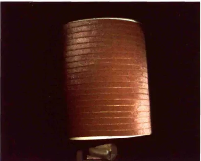
We have extended Matusik's image-based setup to handle anisotropic BRDFs (Figure 2-3). Our extension is similar to the method proposed by Lu et a1. [61, 62], who measure the BRDFs of velvet and shot fabric with a manual setup. Our setup is automated with precision motors. A cylinder is used instead of a sphere as the measurement target so that we can paste material samples on top without distortion. We compensate for the lost degree of freedom in normal variations by mounting the cylinder on a precision motor and performing measurements at different tilt angles. In order to account for anisotropy we cut multiple strips from a planar sample of the material at different orientations. The strips are then pasted onto the cylinder target. Together with the degree of freedom for the light position, we are able to acquire the full 4D BRDF using a large set of two dimensional images. Figure 4-1 shows an example input image of a acquired velvet sample. More details about our measurement will be described in Section 4.3.1.

2.3.2 BTF Measurement

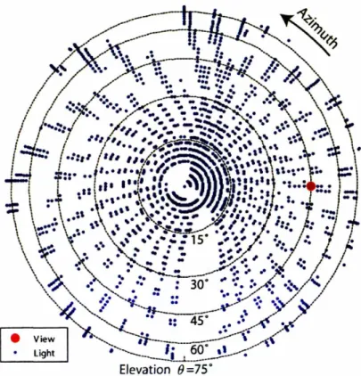
The first BTF measurement device was built by Dana et al. [24]. In this device, a robot arm is used to orient the texture sample at arbitrary orientations, and the camera and light orbit around the sample. 205 combinations of light and view directions are sampled for each material, and more than 60 materials have been measured and published [17]. Due to the sparse sampling, it is not practical to use the measured data for rendering directly. More recently, researchers have built similar setups and provided measurements at higher angular resolutions [97, 51, 38]. Analogous to the gonio-reflectometers for BRDFs, only one sample is measured at a time for a particular lighting and viewing directions, even though each sample is a texture.

MUller et al. [77] present a setup to capture BTFs more efficiently by simultaneously capturing multiple views using multiple cameras. They built a hemispherical gantry con-sisting of 151 consumer digital cameras. The on-camera flashes serve as light sources. By synchronizing the cameras, 151 x 151 = 22801 images can be captured in 151 time steps, and the authors report a measurement time of about 40 minutes. While this is a big improvement in terms of measurement time, the setup is large and costly.

Han and Perlin [41] introduced a measurement setup based on a kaleidoscope, which allows viewing a sample from multiple angles simultaneously through multiple reflections. Illumination is provided by a projector pointing into the kaleidoscope. By selectively il-luminating a small group of pixels, the light direction can be controlled. Since there is no moving part in this setup, measurement is very fast. However, the equipment is difficult to build and calibrate. In addition, due to multiple reflections in the optical path, the result quality tends to be rather low. Dana and Wang [19] proposed a setup based on a parabolic mirror. While their setup can provide higher quality measurements than the kaleidoscope setup, they can only capture a single spatial location at a time. As a result, it does not offer any acceleration compared to the gonio-reflectometer-like approaches.

Due to the nature of spatial variations for BTFs, multiplexing approaches based on curved geometry cannot be directly applied to BTF measurement. Suppose we have a curved sample of the material and the spatial variation is periodic. To map each measured

pixel to the domain of the BTF, we will need to know the texture coordinate the surface point corresponds to, in addition to its normal. Indeed, real textured objects are seldom perfectly periodic, so the correct correspondence can be ill-defined. In Chapter 5, we will present our BTF representation, which avoids the need of precise correspondence. As a result, we are able to build a new measurement setup that allows capturing of multiple texture samples at the same time, even if they are not perfectly identical.

2.3.3 Reflectance Fields

The BSSRDF is defined on a planar geometry (Section 2.1.2). However, its definition can be easily generalized to a general parameterized surface. In this case the BSSRDF is commonly known as a reflectance field. The full reflectance field is a 8D quantity like the BSSRDF, and it is often reduced to lower dimensions by fixing some of the dimensions.

Single View

Many works in reflectance field measurement assume distant illumination: the entire object is lit by parallel rays from a certain direction. This assumption removes the dependency on incident locations. By further restricting the measurement to a single view, the reflectance field can be reduced to 4D, depending only on the surface location and direction of incident light. Debevec et al. [26] built a dome-shaped setup which records the reflectance field of a human face under varying light directions and a fixed view. Similarly, Malzbender et al. [63] have built a hemispherical gantry with 50 lights to capture the single-view reflectance field of small objects. Masselus et al. [67] present a method to lift the distant illumination assumption and acquire a fixed-view 6D reflectance field using a local lighting basis provided by a projector.

Multiple Views

The following works all assume distant lighting. Lensch et al. [56] capture a small number of images of an object under varying light and viewing directions. By assuming that the object can be represented with a small number of distinct BRDFs, they cluster similar

reflectance from different surface locations to improve angular resolution. The clustered BRDFs are then fit to parametric models. Matusik et al. [69, 70] present a system which acquires the reflectance field from multiple viewpoints, using turntables to rotate the object and lights. A relatively sparse sampling of the 6D reflectance field can be captured, but the acquisition process take many hours. Weyrich et al. [121] built a dome with 15 cameras and more than a hundred lights for measuring face reflectance, similar to Debevec's Light Stage. The measurement time is about 15 seconds, making it possible to record live subjects. With this setup, 15 views are captured, providing sparse slices of the 6D reflectance field.

Subsurface Scattering

Jensen et al. [45] propose a model for rendering the BSSRDF by using a dipole approx-imation to a diffusion model. Although the method is limited to homogeneous materials, it has become very popular in the field due to its efficient evaluation and the tremendous improvement in rendering quality. They also introduce a simple method to estimate the diffusion model parameter from a single image. More recently, Goesele et al. [39] present a measurement setup for translucent inhomogeneous objects by using a laser beam as the illuminant. To limit the dimensionality of measurement, their work is limited to diffuse surface reflection. Tong et al. [109] measure subsurface scattering in quasi-homogeneous material by assuming only short distance subsurface scattering is inhomogeneous.

2.4 BRDF Representations

2.4.1

Analytical Models

Many analytical BRDF models have been proposed in the past few decades. They can be roughly divided into two classes: empirical models seek to emulate the characteristics of material reflection qualitatively [6, 118, 52], while physically-based models derive the quantities from first principles of physics [13, 42]. A number of the more well-known models will be listed here. We change the notations for some of the models from their original form for more consistent notation. For further information on the models, the

Table 2.1: Common notations for BRDF models.

reader is referred to the original papers.

In Table 2.4.1 we list the common notations we use for all the BRDF models listed. BRDF is always defined in a local coordinate system -defined by the normal, the tangent and the binormal. A BRDF model is typically composed of two components, the difuse term and the specular term. The diffuse term generally describes the aggregate effects of multiple reflections. As a result, it is mostly independent of the light and view direction. In the ideal case it is Lambertian, i.e. constant for all direction pairs. The specular term generally describes the directional component of reflection. For common materials which are not entirely diffuse, the overall reflection for a particular incident ray has a maximum near the mirror direction. The specular term specifies the location of this peak, together with the falloff surrounding it. For the BRDF models listed here, many of them are focused on the specular term, and either assume a Lambertian diffuse term or do not specify it explicitly. For the Lambertian case, the diffuse term is simply specified by the diffuse color, a separate Pd for each channel. For the specular term, it is generally a nonlinear function of several parameters, scaled by Ps for each channel. The nonlinear parameters are typically the same for all channels. This is not a requirement for physical plausibility, but different parameters per channel will lead to unnatural color shift in most cases.

There are two properties that a BRDF model need to satisfy in order to be physically plausible. First, a BRDF has to be reciprocal: the value of the BRDF should be the same when the incoming and outgoing direction is exchanged [114]. Second, a BRDF has to be

p(L, V) BRDF evaluated at (L, V)

N normal

V, (Vx, Vy, Vz) outgoing vector (view) L, (lx,ly, lz) incoming vector (light)

R mirror reflection of L

H half-way vector between L and V

(Oh, Oh) spherical coordinates of the half vector H

Ps specular lobe scaling factor

energy-conserving, meaning the outgoing energy must be less than or equal to the incoming energy. With the presence of the scalar factors Pd and ps, this can always be achieved for any model. Under a more restrictive definition, a BRDF model is considered energy-conserving if given Pd + Ps = 1, the BRDF is energy-conserving for all possible parameters. Finally, in cases where the incoming and outgoing energy are strictly equal, we call the model strongly energy-conserving.

Phong Model

The Phong model [87] is the most well-known shading model in computer graphics. The core idea is the empirical observation that for specular/glossy materials, the reflection is strongest along the mirror direction R with respect to the light L, with a smooth falloff surrounding R. To describe this falloff, Phong suggests to use the cosine between V and R, raised to a certain power n. The original formulation is:

(V -R)n2

p(L, V) = Pd + Ps - . (2.11)

N-L

The original Phong model is not physically plausible -it does not satisfy energy con-servation or reciprocity. A simple modification that ensure these properties is as follows:

Pd n+2

p(L, V) = d + ps- (V .R)n (2.12)

n

2it

There is a variant of the Phong model proposed by Blinn [6], based on the halfway vector H and surface normal N:

Pd n+2

p(L, V)= R+ Ps_ (H -N)n (2.13)

This variant is also the default shading model implemented in OpenGL. In Chapter 3 we will demonstrate the subtle but important difference between the Blinn version and the original Phong model.

Ward Model

Ward [ 118] proposes an empirical BRDF model that accounts for anisotropy. Instead of the cosine lobe used by Phong, the Ward model is based on the elliptical Gaussian. In addition, the model is defined with respect to the half-vector H. It has two parameters, a and P, that define the spread of the lobe in the two directions. For isotropic materials a = 3 and the Ward model has a single parameter. The formula is as follows:

p(L,V) 1+ps exp [- tan2 Oh(cOS2 Wah/a2 + sin2 h/• 2)] (2.14)

V /(NL)(N -V) 4(arc

The model is reciprocal, a fact immediate from the equation shown. However, recently

Dilr [30] shows that the model is not strongly energy-conserving. He proposes a modifica-tion to the model to make it strongly energy-conserving:

Pd 1 exp[- tan2 Oh(COS2 h/a 2 + sin2 0h/0 2)]

p(L,

V)

= +

Ps

(2.15)

+ (N -L) (N .V) 4nap

Cook-Torrance Model

The Cook-Torrance model [13] is a physically-based model which adopts the microfacet formulation from Torrance and Sparrow [110]. The basic assumption is that the surface is composed of many tiny smooth mirrors. As a result, the reflectance at a particular light/view combination is a function of the number of aligned microfacets, the amount of shadowing and masking between the microfacets, and the reflectance of the ideal mirrors. The formula is as follows:

Pd Ps DGF

p (L, V)= + (2.16)

n ~n (N -L)(N-V)

2(N-H)(N.V) 2(N-H)(N-L) G min{, (V H) (V -H) 1 e- [(tanOh)/m]2 _(2.18) D 2 COS4 Oh

G is the geometric attenuation term which approximates the shadowing and masking effects, while D is the distribution of the microfacets. F is the Fresnel term which governs the reflection for smooth mirrors.

Lafortune

While the work by Lafortune et al. [52] is presented as a non-linear basis for reflectance representation, it is commonly considered as a phenomenological BRDF model as well. The non-linear basis can be seen as a generalized cosine lobe:

B = [Cxlxvx +-Cylyvy +Czlzvz] n (2.19)

This expression is equivalent (within a constant factor) to the cosine lobe used by Phong

when Cx = Cy = -1, Cz = 1. The authors suggest the use of multiple lobes to fit

measure-ment or a physically-based BRDF model. Since its introduction, the Lafortune model has become one of the most popular models because of its generality and computational effi-ciency. However, as we will show in Chapter 3, the model produces unnatural highlights which limits its plausibility for a significant subclass of materials.

Oren-Nayar

Oren and Nayar [83] developed a model that improve upon the common Lambertian diffuse model. Similar to Cook-Torrance, it is also based on a collection of microfacets, but these microfacets are modeled as perfectly diffuse surfaces. However, due to complex shadowing effects, the overall BRDF is not Lambertian. They show that their model matches diffuse objects in the real world much closer than Lambertian. The reader is referred to their paper for the full formulation.

He-Torrance-Sillion-Greenberg Model

The model proposed by He et al. [42] is considered the most comprehensive analytical BRDF model. Unlike most other works, the He model takes polarization and other wave phenomenon into account. The formula for the model is very complex and the reader is referred to the paper for further information. In this thesis, we use the implementation of the unpolarized version of the He model by Rusinkiewicz [95].

2.4.2 Generalized microfacet model

While physically-based models like Cook-Torrance and He are derived based on a micro-facet distribution, they typically put strong assumptions on the shape of this distribution, e.g. Gaussian. These distributions are typically controlled by one or two parameters only. Ashikhmin et al. [1] introduced a method to create a BRDF from an arbitrary distribution of microfacets.

The expression for the Ashikhmin et al. model is as follows: p(LV) = p(H)(H .N)F(L- H)

4g(L)g(V)

where p(H) is the microfacet distribution; g(-) is the shadowing/masking term; F(L -H) is the Fresnel term for the mirrors aligned with H; and (-) denotes the average over the distribution p. The model will be explained in more detail in Chapter 4, where we also present a method to estimate the microfacet distribution from measured data.

2.4.3 Data-driven Representations

To overcome the limitations of analytical models, a data-driven approach considers the BRDF as a fully general 4D function. By exhaustive sampling of the 4D domain, it is theoretically possible to represent any BRDF. However, in practice, this representation is limited by the measurement resolution and noise. In addition, it requires significant storage and is difficult to edit.

example, Westin et al. [119] propose the use of spherical harmonics to store anisotropic BRDF data. Theoretically, spherical harmonics can encode any function on the hemisphere, but many coefficients will be necessary for functions with high angular frequencies. As a result, representations based on spherical harmonics are only efficient for relatively diffuse BRDFs. Schroeder and Sweldens [100] propose spherical wavelets to represent a 2D slice of the BRDF by fixing one of the direction. Lalonde and Fournier [53] use a wavelet coef-ficient tree to represent full BRDFs. Other representations based on compression include Zernicke polynomials [50], singular value decomposition[48] and positive matrix factor-ization [74].

2.5

Spatially-Varying Reflectance

2.5.1

Approximations

A number of techniques have been proposed in the past to approximate spatially-varying reflectance with different levels of simplification. The most primitive example is standard texture mapping, where different surface locations map to different colors. Bump map-ping [7] simulates the effect of surface roughness by perturbing surface normals. Horizon mapping [72, 105] enhances bump mapping by handling self shadowing effects. Heidrich et al.[44] further improves microgeometry rendering by efficient interreflection estimation using precomputed visibility. The displacement map [12] is typically not considered a re-flectance technique since it changes the underlying geometry. However, recent extensions [116, 117] to the displacement map are applied at shading time. Occlusion and shadow-ing are precomputed to allow for interactive rendershadow-ing. While the above techniques offer different traoffs between computation cost and quality, they all depend on accurate de-scriptions of the microgeometry which are unavailable and often difficult to acquire from real materials in most cases. As a result, these techniques are often only applied to render synthetic materials.