HAL Id: hal-02940070
https://hal.inrae.fr/hal-02940070
Submitted on 16 Sep 2020
HAL is a multi-disciplinary open access
archive for the deposit and dissemination of
sci-entific research documents, whether they are
pub-lished or not. The documents may come from
teaching and research institutions in France or
abroad, or from public or private research centers.
L’archive ouverte pluridisciplinaire HAL, est
destinée au dépôt et à la diffusion de documents
scientifiques de niveau recherche, publiés ou non,
émanant des établissements d’enseignement et de
recherche français ou étrangers, des laboratoires
publics ou privés.
Distributed under a Creative Commons Attribution| 4.0 International License
Danielle Dias, Allan Pinto, Ulisses Dias, Rubens Lamparelli, Guerric Le
Maire, Ricardo da S Torres
To cite this version:
Danielle Dias, Allan Pinto, Ulisses Dias, Rubens Lamparelli, Guerric Le Maire, et al.. A
Multi-Representational Fusion of Time Series for Pixelwise Classification. IEEE Journal of Selected Topics
in Applied Earth Observations and Remote Sensing, IEEE, 2020, 13, pp.4399-4409.
�10.1109/JS-TARS.2020.3012117�. �hal-02940070�
A Multi-Representational Fusion of
Time Series for Pixelwise Classification
Danielle Dias, Allan Pinto, Member, IEEE, Ulisses Dias, Rubens Lamparelli, Guerric Le Maire, and Ricardo da
S. Torres, Member, IEEE
Abstract—This paper addresses the pixelwise classification problem based on temporal profiles, which are encoded in two-dimensional representations based on Recurrence Plots, Gramian Angular/Difference Fields, and Markov Transition Field. We propose a multi-representational fusion scheme that exploits the complementary view provided by those time series rep-resentations, and different data-driven feature extractors and classifiers. We validate our ensemble scheme in the problem related to the classification of eucalyptus plantations in remote sensing images. Achieved results demonstrate that our proposal overcomes recently proposed baselines, and now represents the new state-of-the-art classification solution for the target dataset. Index Terms—Pixelwise classification, classifier fusion, time series representation, eucalyptus
I. INTRODUCTION
P
IXELWISE remote sensing image classification has beenestablished as an active research area. Proposed solutions have been validated in relevant applications, including among others ecological studies [1], [2], phenology analysis [3]–[7], land-cover change monitoring [8], and crop identification [9]. A promising research venue relies on the development of classification systems based on time series associated with pixels (e.g., time series associated with vegetation indices, such as normalized difference vegetation index – NDVI – or enhanced vegetation index – EVI). Often, such methods assume that pixels can be categorized into different classes based on time series patterns, also refereed to as temporal profiles.
Danielle Dias is with Institute of Computing, University of Campinas (Unicamp), Campinas, Brazil. Email: [email protected].
Allan Pinto is with Institute of Computing and School of Physical Ed-ucation, University of Campinas (Unicamp), Campinas, Brazil. Email: [email protected].
Ulisses Dias is with School of Technology, University of Campinas (Uni-camp), Limeira, Brazil. Email: [email protected].
Rubens Lamparelli is with N´ucleo Interdisciplinar de Planejamento En-erg´etico, Unicamp, Campinas, Brazil. Email: [email protected]. Guerric le Maire is with Eco&Sols, CIRAD, Univ Montpellier, INRA, IRD, Montpellier SupAgro, Montpellier, France. Email: guerric.le [email protected]. Ricardo da S. Torres is with the Department of ICT and Natural Sciences,
Norwegian University of Science and Technology (NTNU), ˚Alesund, Norway.
Email: [email protected]
Authors are grateful to CNPq (grant #307560/2016-3), S˜ao Paulo Research Foundation – FAPESP (grants #2014/12236-1, #2015/24494-8, #2016/50250-1, #2017/20945-0, and #2019/16253-1) and the FAPESP-Microsoft Virtual Institute (grants #2013/50155-0, and #2014/50715-9). This study was financed in part by the Coordenac¸˜ao de Aperfeic¸oamento de Pessoal de N´ıvel Superior - Brasil (CAPES) - Finance Code 001.
Corresponding author: Ricardo da S. Torres (e-mail:
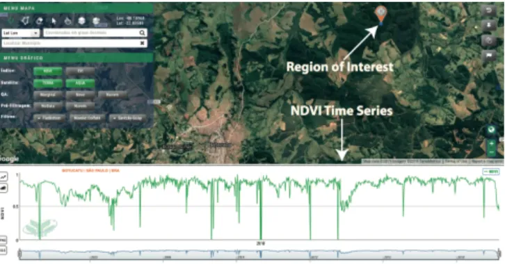
Fig. 1. Example of the NDVI time profile for a coordinate selected as a
region of interest in satellite images.
Fig. 1 shows an example of the temporal profile of the
NDVI of a region in Botucatu, S˜ao Paulo, Brazil.1 The figure
indicates a region of interest where a pixel is selected to compute the NDVI values in relation to time. The time series in the bottom is obtained from NDVI values.
The construction of pixelwise classification systems usually demands the definition of suitable extractors to encode tempo-ral profiles into feature vectors; and effective classifiers, which learn from extracted features how to assign samples (pixels) to the correct category. Several approaches have been proposed to address both problems separately, and altogether.
One promising approach recently employed in the literature refers to the use of intermediary representations to encode time series properties [10], [11]. In particular, a promising family of methods relies on the use of two-dimensional representa-tions [7], [12], [13], which can be transformed into images. The goal of such approaches is to benefit from successful computer vision methods proposed for image classification, to more effectively classify time series [4], [7], [14]–[16].
Examples of successful two-dimensional representations in-clude Recurrence Plot (RP) [13], Gramian Angular/Difference Fields (GASF/GADF) [12], and Markov Transition Field (MTF) [12]. RP has been extensively used to represent nonlinear patterns of dynamic systems, through the compu-tation of the autocorrelation for different time scales [13]. GASF/GADF [12] representations encode in polar coordinates time series properties preserving temporal relations, while the MFT [12] captures the transition probabilities among different time series states.
1Source: SATVeg system, Embrapa, Brazil – https://www.satveg.cnptia.
RP, GASF/GADF, and MTF have been successfully vali-dated in pixelwise classification and search tasks through the characterization of pixel-related time series (e.g., vegetation indices) associated with sequences of images [14]–[17]. In part, the success of those initiatives is due to the use of effective state-of-the-art data-driven feature extractors [18]– [24]. In [14], [15], for example, ten different deep-learning feature extractors were investigated in combination with RP, GASF/GADF, and MTF representations. Remarkable results were achieved in pixelwise classification problems.
Would the combination of multiple representations, data-driven feature extractors, and classifiers lead to even better pixelwise classification results? This is the question that guides the research described in this paper. We introduce a multi-representational fusion approach for exploiting the comple-mentary view of multiple classification systems constructed using different representations and feature extractors.
In our fusion scheme, the importance of different classifiers are assessed based on the Gini index [25], a metric computed on the training of a random forest classifier, and on the bal-anced accuracy scores [26] of different predictors. Classifiers are ranked, and the top-k ones are used to define lists with complementary classifiers, defined in terms of the Kappa’s coefficient [27]. Classifiers found in multiple lists are used to train an SVM-based meta classifier, producing the final prediction model. To the best of our knowledge, this is the first work dedicated to the investigation of the fusion of classifiers based on multiple time series representations.
We validate the proposed approach in the problem related to the identification of eucalyptus plantations in remote sensing images. Achieved results are consistently better than recently proposed approaches validated on the same dataset, as well as traditional ensemble approaches proposed in the literature.
This article is organized as follow. Section II introduces background concepts related to the employed time series representations. Section III provides an overview of related work. Section IV describes the proposed fusion scheme. The adopted experimental protocol is presented in Section V. Achieved results are presented and discussed in Section VI. Finally, Section VII summarizes our findings, as well as points out some possible research directions for future work.
II. BACKGROUNDCONCEPTS ONIMAGE
REPRESENTATIONS
In this work, we encode the temporal profile of pixels ex-tracted from remote sensing images representing the temporal characteristics as 2D images. The values of the vegetation indices of the pixels are grouped together as time series and undergo transformations in such a way that the one-dimensional series is represented as a two-one-dimensional matrix. That said, we can use this matrix as an input image for feature extractors. This is the rationale of our work. To achieve this goal, we investigate three approaches that encode time series as image representation.
1) Recurrence Plot: Recurrence Plot – RP [13] is a tool
for visualizing the recurrent behavior of a trajectory in the
phase space in dynamic systems. Let T = (t1, t2, . . . , tn)
be a time series with n observations, the recurrence plot representation encodes every time the trajectory of T visits approximately the same area in the phase space. A graphical representation of recurrence plot is an image formed by a matrix of dimension n × n. The generated image is a direct representation of the distance matrix, that is, the information contained in the recurrence plot is the proximity value of each pair of subsequences in the trajectory of the time series [28]. The two-dimensional representation of T is the matrix M ,
where each cell Mi,j is computed by the distance function
f (Ti, Tj)|∀i, j ∈ {1, 2, . . . , n}. The function f encodes how
recurring are the time series states. In this paper, the construc-tion of the recurrence plots is based on three implementaconstruc-tions of the function f [14], [16]: difference (DIF), division (DIV), and multiplication (MULT).
f (Ti, Tj)DIF = |Ti− Tj| (1) f (Ti, Tj)DIV = Ti Tj (2) f (Ti, Tj)M U LT = Ti× Tj (3) Fig. 2 is an example of recurrence plots. In this example, two NDVI time series are provided. The dark green time series is associated with a pixel from an eucalyptus region, while the orange time series is from a noneucalyptus region. First, the n time series observations are used to construct the matrices DIF, DIV, and MULT, following Equations 1, 2, and 3, respectively. Then, a normalization step is performed so that the resulting values range from 0 to 255, which enables the creation of images in gray level.
We also create an additional representation using the three grayscale images as channels of an RGB image. In this representation, the MULT, DIV, and DIF matrices, in this order, are used to form the channels of the red, green, and
blue bands, respectively. In the end, the representations are
the recurrence plots DIF, DIV, MULT, and RGB, for each time series provided.
2) Representations GAF: Gramian Angular Field (GAF)
is another approach to encode time series as images. It was proposed by Wang & Oats [12], and it is inspired by the notion of Gramian matrices from the linear algebra field.
Let us assume we have a real vector space of finite di-mension with inner product. The Grammar matrix of a set of vectors is computed by the inner product of pairs of vectors. The inner product between two vectors can be calculated by the norm of the vectors (also called modulus, magnitude or intensity) and the angle between them. From a geometric point of view, the module corresponds to the length of the vector. Let u and v be two vectors, the internal product between them is given by:
hu, vi = kuk · kvk · cos(φ). (4)
If u and v have norms equal to 1, then the equation can be simplified:
0.444 0.444 0.4710.471 0.4290.429 T1 - T1T1 - T2 ... T1 - Tn T2 - T1T2 - T2 ... T2 - Tn ... ... Tn - T1Tn - T... 2 ... Tn - T... n RP - DIF T1 / T1T1 / T2 ... T1 / Tn T2 / T1T2 / T2 ... T2 - Tn ... ... Tn / T1Tn / T... 2 ... Tn / T... n RP - DIV T1x T1T1x T2 ... T1x Tn T2x T1T2x T2 ... T2 - Tn ... ... Tnx T1Tnx... T2 ... Tnx... Tn RP - MULT 0.767 0.767 0.8060.806 0.8340.834 T1 T2 Tn ... ... ... T1x T T1T1x T T2 ... T1x T Tn T2x T T1 ... Tnx T T1 T1 - T1T1 - T2 ... T1 - Tn T2 - T1 ... Tn - T1 T1 / T / T1T1 / T / T2 ... T1 / T / Tn T2 / T / T1T2 / T / T2 ... T2 - T - Tn ... ... Tn / T / T1Tn / T / T2... ... Tn / T / Tn... G = Dif R = Mult B = Div RP - RGB RP EucalyptusRP Noneucalyptus
Fig. 2. Example illustrating the creation of recurrence plot matrices for
distance functions DIF, DIV, and MULT.
Let {v1, v2, . . . , vn} be a set of n vectors, the G Gramian
matrix is a square n × n matrix such that every cell gi,j =
hvi, vji: G = hv1, v1i hv1, v2i . . . hv1, vni hv2, v1i hv2, v2i . . . hv2, vni .. . ... . .. ... hvn, v1i hvn, v2i . . . hvn, vni . (6)
Considering that all n vectors have norm 1, then the inner product is given by the cosines of the angle between the vectors (Equation 5). Therefore, the Gramian matrix is formed by: G =
cos(φ1,1) cos(φ1,2) . . . cos(φ1,n)
cos(φ2,1) cos(φ2,2) . . . cos(φ2,n)
..
. ... . .. ...
cos(φn,1) cos(φn,2) . . . cos(φn,n)
(7)
where θi,j is the angle between vectors i and j.
GAF uses ideas of Gramian matrices to represent a series of observations into a matrix that contains temporal correlation between observations in different time intervals. Wang & Oats [12] created two GAF representations: Gramian differ-ence angular field (GADF) and Gramian summation angular field (GASF). GADF is a Gramian matrix in which each element is the trigonometric difference between each pair of
2000 2002 2004 2006 2008 2010 2012 2014 2016
Normalized Time Series
Time Series in Polar Coordinates
GADF
GASF
Fig. 3. Example illustrating the creation of the GADF and GASF represen-tations.
time intervals, while the elements of the GASF matrix are formed by the trigonometric sum.
Let T = (t1, t2, . . . , tn) be a time series. We need to
perform trigonometric operations, that is, the n observations need to be transformed into angles. To achieve this, first the time series T is normalized in the interval [−1, 1], resulting
in ˜T = ( ˜t1, ˜t2, . . . , ˜tn). After that, the time series coordinate
system (Cartesian coordinates) is transformed into polar
coor-dinates system computing the angular cosine of each ˜T value:
φi= arccos( ˜ti), ˜ti∈ ˜T . (8)
After obtaining the angles and inspired by the idea of Gramian matrices, the trigonometric difference and the trigonometric sum between each point is considered for the creation of the GADF and GASF matrices, respectively:
GADFi,j= sin (φi− φj) (9)
GASFi,j= cos (φi+ φj) (10)
Fig. 3 illustrates the creation of the GADF and GASF representations. In this example, we consider a time series with NDVI values associated with a pixel from an eucalyptus region. First, the n observations from the time series are normalized and the time series is transformed into a polar coordinate system (Equation 8). After that, we created the GADF and GASF matrices, according to Equations 9 and 10, respectively. Then, we normalized the values between 0 and 255 to allow the creation of gray level images.
GADF and GASF representations preserve temporal depen-dencies. An observation in the time period i is compared with an observation in the time period j and the time increases when traversing the matrix from the upper left corner to the lower right corner. This creates patterns in the matrix, which also reflects in the image representation created.
3) Representation MTF: Markov Transition Field (MTF) is another representation proposed by Wang & Oats [12] to encode time series as images. MTF captures state transition statistics and encodes these statistics as an image.
Let T = (t1, t2, . . . , tn) be a time series with n
observa-tions. First, the set of all possible values of the time series are divided into a fixed number of states. This is accomplished by compartmentalizing the time series in Q quantile bins and assuming that each compartment is a state. Thus, we create
ˆ
T = ( ˆt1, ˆt2, . . . , ˆtn) that is, ˆti is the quantile to which ti is
associated.
We create the intermediate matrix WQ×Q, where wi,j is
the number of times that transitions from the state i to the state j occur. Then, we perform a normalization so that each row of the W matrix has sum equal to 1. Thus, W stores the probabilities of state transitions and it is considered the first order Markov transition matrix, in which the lines indicate the probability of state transitions, the columns indicate the time dependency, and the main diagonal captures the probability of staying in a given state.
Finally, we created the MTF matrix (Markov Transition Field) considering the time position of T , with dimensions n × n, where the each cell in the MTF matrix indicates the probability of undergoing transition from the state associated
with Ti to the state associated with Tj. The MTF matrix is
constructed as follows: M T F = Wtˆ1, ˆt1 Wtˆ1, ˆt2 . . . Wtˆ1, ˆtn Wtˆ2, ˆt1 Wtˆ2, ˆt2 . . . Wtˆ2, ˆtn .. . ... . .. ... Wtˆn, ˆt1 Wtˆn, ˆt2 . . . Wtˆn, ˆtn . (11)
Fig. 4 shows an example of creating the MTF representation. In this example, we receive a time series with NDVI values associated with a pixel from an eucalyptus region. First, the n observations in the time series are divided into quantiles or states. In this example, we define Q = 5 to create five states represented by colors in the time series. Then, we count how many transitions occur between states and create the preliminary W matrix. We then normalize W to make it the first order Markov transition matrix.
We build the MTF matrix according to Equation 11, then we normalize the values between 0 and 255 and finally convert the MTF matrix into an image.
An important characteristic of MTF matrices is that the transition probabilities are coded in several stages in a single
representation. For example, M T Fi,j such that |i − j| = 1
represents the transition process along the time axis with a unit of difference. If we make |i − j| = 2, then we have the transition process within two units of time, and so on. The main diagonal represents the probability of staying in a given state.
III. RELATEDWORK
Existing literature in the area of remote sensing image classification is vast. Most of those initiatives include the the investigation of machine learning algorithms in problems related to the classification and recognition of objects. For an
2000 2002 2004 2006 2008 2010 2012 2014 2016
Fig. 4. Example of creating the MTF representation.
in-depth overview of recent initiatives, the reader may refer to [29]. In this section, we focus on describing studies related to the use of time series in classification problems.
Almeida & Torres [2] used NDVI time series obtained from MODIS sensors. The authors proposed a genetic program-ming (GP) approach for discovering near-optimum combina-tions of time series similarity funccombina-tions. Those funccombina-tions were then used for classifying eucalyptus plantations. Menini et al. [16] also addressed the same problem. Again, a GP ap-proach was used, now for combining similarity scores defined in terms of texture descriptors extracted from recurrence plot representations. The methods proposed in [2] and [16] are considered as baselines, which do not take into account data-driven features in the time series classification task, in our work.
Hu et al. [30] utilized data from MODIS sensors and time series associated with five different vegetation indices. Their work proposed a method to select automatically spatiotem-poral features named Phenology-based Spectral and Temspatiotem-poral
Feature Selection– PSTFS. PSTFS features are then submitted
to a multiclass SVM classifier, used to determine to which crop a particular sample belongs. Different from our approach, that work did not exploit time series representations.
Liu et al. [31] exploited Landsat-8 images and the
Uni-versal Normalized Vegetation Index – UNVI [32], an index
that encodes information from all observed bands. In their study, UNVI is compared with other vegetation indices and effective results are reported. The use of UNVI time series in combination with a random forest classifier was effective in a five-class classification problem. No time series representation was employed as well.
Another research venue concerns the proposal of approaches for combining patterns found in time series associated with vegetation indices with spectral information, as in [33]. In that study, classifiers, such as random forest and SVM, were explored in problems related to the classification of multiple crops. Special time series representations were not investigated in that work.
pixelwise- and object-based classification methods. One rel-evant representative is the work of Belgiu et al. [8]. In their work, NDVI time series were categorized based on the use of a random forest classifier and the Time-Weighted Dynamic Time
Warping (TWDTW) [8]. Even the combination of
pixelwise-and object-based approaches have already been investigated, as in the work of Rahimizadeh et al. [34]. In their work, the forest classification problem was addressed by the combination of a time series classifier – using SVM and vegetation indices – and an object-based classification approach based on forest structural patterns. These studies suggest that the investigation of pixelwise classification approaches are an active research area, which can even be exploited in combination of object-based approaches. We plan to address that, in the context of the use of time series representations, in future work.
Another family of methods has focused on the classification of time series associated with vegetation indices extracted from images obtained from near-surface sensors [35], [36]. The work of Almeida et al. [5], for example, investigated the use of a multiscale classifier based on AdaBoost. In that work, time series were used as input feature vectors of the considered classifiers. In [37], the authors also addressed a fusion problem, in that case based on the combination of time series associated with multiple vegetation indices. A GP-based approach was exploited and the focus was on the retrieval of time series, instead of their classification. In another work [3], time series associated with pixels were classified though the use of an SVM meta classifier [38]. Almeida et al. [6] also investigated the use of unsupervised fusion schemes but in the context of retrieval tasks. In none of those works, time series representations were explored.
Two-dimensional representations were investigated in time series classification and retrieval problems in [4], [7]. In [7], the phenological visual rhythm was introduced to encode veg-etation phenology changes into images. Traditional color de-scriptors are employed in the characterization of such images. In [4], both recurrence plot and visual rhythm representations were explored in the context of a pixelwise classification fusion problem. Different from our approach, however, no data-driven features were used.
IV. PROPOSEDAPPROACH
A. Predictors
Before discussing our fusion scheme, we describe in this section the strategy used to construct multiple representations from data. This involves some steps: (i) transformation of time series into representations of images; (ii) use of automatic feature extraction techniques, and (iii) creation of predictors.
First, the time series are encoded in representations of recurrence plot, GADF, GASF and MTF, as described in Section II. We work with individual representations and we also combine matrices in RGB channels. Therefore, we create two RGB representations: (i) an RGB representation composed of MULT, DIF and DIV; and (ii) an RGB representation composed of GADF, GASF, and MTF. These are the orders of the red, green and blue channels, respectively.
Next, we extract features from these image repre-sentations using ten deep convolutional neural networks:
DenseNet121 [18], DenseNet169 [18], DenseNet201 [18], In-ceptionResNetV2 [19], InceptionV3 [20], MobileNetV1 [21], ResNet50 [22], VGG16 [23], VGG19 [23] e XceptionV1 [24]. We use the well-known transfer learning mechanism, in which the last layer of the neural network is removed and the result obtained corresponds to the feature vectors produced by the previous layers.
In addition to the feature vectors extracted from the images, and from the two RGB representations, we also analyze some vector concatenations, such as: DIF DIV, DIF MULT, DIV MULT, DIF DIV MULT (called 3RP), GADF GASF (called COMB2), and GADF GASF MTF (called COMB3).
Finally, we trained four classifiers with the feature vectors: logistic regression, multilayer perceptron (MLP), Na¨ıve Bayes, and support vector machine (SVM). In this way, we create predictors in multi-representational way, where each predictor comes from three elements: the image representation, the deep neural network, and the classifier where it was trained on.
B. Fusion Approach
This section describes our methodology for pixelwise re-mote sensing image classification. Our methodology takes advantage of complementary information among image rep-resentations described in Section II, which were extracted from time series and designed for the remote sensing image classification purpose [14], [15].
To achieve our goal, we adopted the use of a fusion method able to find complementary information among the classifiers investigated in this work. We believe that a fusion approach can lead to gains in terms of balanced accuracy since we have several representations of time series which explore different temporal characteristics of NDVI extracted from eucalyptus pixels. Taking into account that (i) the representations of recurrence plot encode the recurrence in the time series; (ii) the GADF and GASF representations encode static information [12]; and (iii) the MTF representation encodes dynamic infor-mation [12]; we assessed that the classifiers that used these representations can be potentially complementary. Therefore, we hypothesize that the use of representations that explore different characteristics of time series induces a complemen-tarity at the level of classification. The investigation of this hypothesis was conducted using a meta-fusion method, as described in Fig. 5.
In our methodology, we adopted the use of a meta-fusion approach originally proposed for the presentation attack detec-tion problem in biometric systems [39]. Although this method was proposed to fuse classifiers built for a different problem, we believe that the main idea of this approach fits with our problem since we also have multiple views, or representations, from the input images. In the context of this paper, the fusion method aims at building a model from classifiers built using multiple representations. These multiple representations, in turn, are devised from representations of intermediate images that encode different properties of the time series, such as (i) recurrence information; (ii) trigonometric difference between each pair of time intervals; and (iii) probability of state transition. Finally, these intermediate representations are used
P1 P P2 . . . P . . . Pn
0 0 . . . 1 1 0 . . . 0 0 1 . . . 1 1 1 . . . 1 . . . . . . . . .
Training Set Selection of Most
Relevant Classifiers (Gini Importance or Balanced Accuracy) Top-k Most Relevant Classifiers Selection of Most Complementary Classifiers (Cohen’s Kappa) 1 2 3 k . . .
K lists containing the most complementary classifiers to the most relevant Top-K Metaclassifier Training (SVM) Inference P1 1 . . . 01 P P2 . . . P . . . Pn 1 0 . . . 0 1 1 . . . 1 . . . . . . . . . Test Set (a) (b) (c) (d)
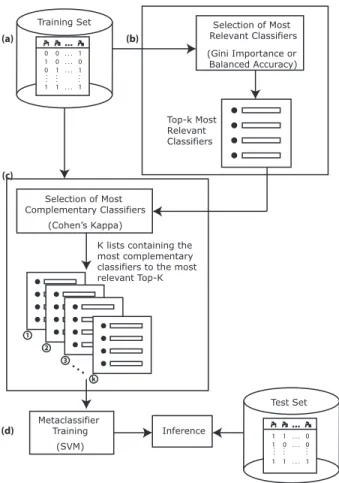
Fig. 5. Overview of the fusion method.
to build classification methods based on extractors of deep learning characteristics, which are used in the fusion process. In summary, the proposed methodology investigated in this work fuses the results of trained classifiers with different image representations, which encode different properties of the time series, consolidating the classification into a single prediction. Fig. 5 presents a general scheme of the multi-representational meta-fusion.
In Fig. 5(a) the method uses the training data of the four predictors (logistic regression, MLP, Na¨ıve Bayes, and SVM), with the views of all the image representations investigated in this work, whose extraction of characteristics were carried out with ten different deep convolutional neural networks. We consider all predictors, since while some may provide complementary views, others can be highly correlated.
To find the most important classifiers, in Fig. 5(b) we used two indices as criteria to estimate the importance of the classifiers: (i) the Gini [25] index, which describes the average reduction in forest impurity and is directly related to decision that random forest uses to select the best available split; and (ii) balanced accuracy of predictors. The Gini index is a measure used by the Random Forest algorithm to infer the importance of variables or nodes (in our case, the classifier). During the training of a Random Forest classifier, the decision trees that composes the Random Forest try to form nodes with a high proportion of data points form a single class, which is achieved by finding the variables that cleanly divide the
training data into classes. For this, the Random Forest can use the Gini index as metric to evaluate the level of impurity for a given node. This value is then used to decide if a node should be split, or not.
In the selection with the Gini index, the training predictors are sent to the random forest algorithm, which randomly generates multiple decision trees from different subsets of the provided predictors. At the end of the random forest training process, the method sorts the classifiers according to their respective importance in the construction of the meta-classification model. At the end of the most relevant selection phase, the meta-classification model is discarded and an ordered list with the top-k classifiers is used in the next step. To find the most complementary classifiers, in Fig. 5(c) the top-k most relevant classifiers are compared with the other predicted classifiers using Kappa’s concordance coefficient as suggested by Cohen [27]. Cohen’s Kappa is a statistical tool to measure the inter-rate agreement between two raters. This method has been applied in several works as toward inferring a confident measure of concordance between two raters. In the context of this work, the Cohen’s Kappa is used to measure the concordance between pairs of classifiers, which can be determined following the reliability reference values: 0.2 < k ≤ 0.4 as fair; 0.4 < k ≤ 0.6 as moderate; 0.6 < k ≤ 0.8 as substantial; and k > 0.8 as almost perfect [40]. Thus, we have k lists containing the classifiers most complementary to the most relevant k classifiers. Finally, classifiers that appear on two or more lists are selected as candidate classifiers, which are used to build a meta-classifier.
To carry out the training of the meta-classification, in Fig. 5(d) we use the SVM algorithm. With the result of the meta-fusion, we make the inference with the test set. All parameters of the fusion method are estimated during training with grid search.
V. EXPERIMENTALSETUP
This section described the evaluation protocol adopted. A. Dataset of Areas with Eucalyptus
The eucalyptus dataset has the MODIS sensor as its source of information, with a combination of the Aqua and Terra satellites in order to reduce the temporal gap and achieve high temporal resolution. We obtained 385 images from Terra (MOD13Q1.005) and 330 images from Aqua (MYD13Q1.005), from February 2000 to November 2016. Both products already provide the computation of the NDVI. MODIS products have 250m spatial resolution, and are pro-duced with 16 days of composition. MODIS have daily records, but only products with a best quality are selected to represent the composition period. Another filtering is per-formed to select only pixels with the same classification label. We used a modified subset of the collection used in le Maire et al. [9]. The selected pixels belong to the eucalyptus and noneucalyptus classes. This dataset is composed of 250 eucalyptus pixels and 1000 noneucalyptus pixels randomly selected. To investigate the impact of noneucalyptus sample unbalancing, we divided the dataset into three sample sizes:
250, 500 and 1000. These values correspond to the number of pixels labeled as noneucalyptus. In each sample we add the 250 eucalyptus pixels.
B. Baselines
This section presents a brief description of the baseline algorithms for fusing classifiers.
1) Majority Vote: The majority vote is the simplest strategy
for fusing information from different sources. This approach assumes that all classifiers have equals importance, and the final decision is determined by the most frequent class (or label output) taking into consideration the classifiers’ output. Given a (n × c) binary matrix L, as follow:
L = d(1,1) d(1,2) . . . d(1,c) d(2,1) d(2,2) . . . d(2,c) .. . ... . .. ... d(n,1) d(n,2) . . . d(n,c) ∈ {0, 1} (12)
where n is the number of inputs, c is the number of classifiers,
and d(n,c)is the label output of the c-th classifier for the n-th
input. Thus, the ensemble decision Ψ = [ω1, · · · , ωn] for the
n input samples are determined as follow:
Ψ = max j∈{0,1} c X k=1 δ(d(n,k), j) (13)
where δ(i, j) is defined as 1 if i = j and 0 if i 6= j.
2) AdaBoost: Adaptive Boosting (AdaBoost) [41] aims to
combine multiple ‘bases’ classifiers to produce an ensemble decision with a performance better than any of the bases classifiers. Boosting approaches perform the training phase of base classifiers in sequence and using a weighted scheme of the data whose weighting coefficient of each data point depends on the performance of the previous classifiers [42]. In particular, the AdaBoost algorithm initially set an equal weight for the data point as 1/n, where n is the size of the data, and at each stage of the algorithm the weighting coefficients are increased for those data points that was misclassified by the previously trained classifier. After the bases classifiers have been trained, they are combined to produce an ensemble de-cision using coefficients that give different weight to different base classifiers.
3) Gradient Boosting: Gradient Boosting is an extension
of AdaBoost to regression problem [43]. Different from Ad-aBoost algorithm, the Gradient Boosting learns via residual errors, instead of using the weighting coefficients computed for each data point. While the AdaBoost algorithm mines the hard data samples by updating the weighting coefficients according to bases classifiers’ response, the Gradient Boosting algorithm does the same thing by using gradients computed upon the loss function. Thus, the loss function is used to infer how good the model’s coefficients are at fitting the data. In this work, we adopted the use of negative binomial log-likelihood loss function, which provides probability estimates, and decision trees as base classifiers.
4) Random Forest: Random forest is a machine learning
algorithm composed of multiple decision trees built on differ-ent random subsets of the training data. The training strategy adopted by this algorithm is known as boost strapping (or bagging) which aims to reduce the variance of the bagged model and to help avoiding over-fitting. Given a set of decision tree classifiers (base classifiers), the bagging strategy splits the data randomly, with replacement, which are used to fit the base classifiers in an independent manner. After training, the bagged model is computed by taking the majority vote of base classifiers. To estimate the performance of the individual trees, a subset of the training data, called out-of-bag (OOB) samples, is separated from the training data and used to estimate the generalization error of the bagged model. The OOB samples is also used to compute the error rate of all variables infer the feature importance.
5) Fusion of Classifiers via Support Vector Machine:
Sup-port Vector Machine (SVM) algorithm has been successfully employed for fusing information for the different classification problems due to strong generalization capability when its parameter values were chosen accordingly. The training stage of an SVM classifier in the context of fusion of classifiers is given as follows. Given a (n × c) binary matrix L that gathers the label outputs of c classifiers for the n input samples from the training set, the ensemble decision of a set of classifiers c is performed by feeding an SVM algorithm with L matrices to fit a classification model or ensemble model. During the training stage, we applied a grid search and k-fold cross-validation protocol to estimate the parameters C and γ since we use the radial basis function (RBF) as a kernel. After estimating an SVM-based ensemble model, the testing phase is performed by running c classifiers on the p testing samples, whose labels outputs are gathered to build a (n × p) binary matrix H. Next, the H matrix is used to feed the SVM-based ensemble model that produces the final label output for each testing sample p.
C. Evaluation Protocol
We conducted the experiments and evaluation of the pro-posed method using the MODIS sensor images with eu-calyptus pixel samples (see Section V-A). We adopted the same evaluation protocol as Menini et al. [16] to have a fair comparison with our baseline methods. Thus, we divided the dataset into two sets, training set (80%) to train and validate the classification models and the testing set (20%) used only to report the final results of our proposed methods and baselines. We validate classification models by using the k-fold cross validation protocol, with k = 5, and ten replications. The replications is necessary to avoid a biased result since we split the original dataset in a 80%–20% ratio. Finally, the evaluation metric used to measure the performance results of the classifiers was the average of balanced accuracy of ten replications.
VI. EXPERIMENTALRESULTS
TABLE I
COMPARISON OF PERFORMANCE RESULTS,IN TERMS OF MEAN AND STANDARD DEVIATION OF BALANCED ACCURACY,BETWEEN THE BEST CLASSIFIER,
FOR EACH NUMBER OF NONEUCALYPTUS EXAMPLES,TRAINED WITH DEEP REPRESENTATIONS(FIRST THREE ROWS)AND BASELINE METHODS FOR DETECTING EUCALYPTUS AREA(LAST TWO ROWS).
Noneucalyptus Sample Size
Deep Features 250 500 1000
SVM ResNet50COMB3 0.978 ± 0.013 0.958 ± 0.012 0.938 ± 0.021
SVM DenseNet201COMB3 0.974 ± 0.011 0.964 ± 0.014 0.939 ± 0.020
Na¨ıve Bayes InceptionV3COMB3 0.961 ± 0.020 0.960 ± 0.020 0.954 ± 0.012
Menini et al. [16] 0.952 ± 0.005 0.943 ± 0.007 0.921 ± 0.005
Almeida et al. [2] 0.936 ± 0.009 0.938 ± 0.010 0.916 ± 0.016
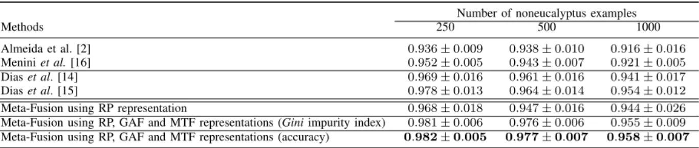
TABLE II
COMPARISON OF PERFORMANCE RESULTS,IN TERMS OF MEAN AND STANDARD DEVIATION OF BALANCED ACCURACY,BETWEEN THE BASELINE METHODS(FIRST FOUR ROWS)AND OUR PROPOSED METHOD(LAST THREE ROWS).
Number of noneucalyptus examples
Methods 250 500 1000
Almeida et al. [2] 0.936 ± 0.009 0.938 ± 0.010 0.916 ± 0.016
Menini et al. [16] 0.952 ± 0.005 0.943 ± 0.007 0.921 ± 0.005
Dias et al. [14] 0.969 ± 0.016 0.961 ± 0.016 0.941 ± 0.017
Dias et al. [15] 0.978 ± 0.013 0.964 ± 0.014 0.954 ± 0.012
Meta-Fusion using RP representation 0.968 ± 0.018 0.947 ± 0.016 0.944 ± 0.026
Meta-Fusion using RP, GAF and MTF representations (Gini impurity index) 0.981 ± 0.006 0.976 ± 0.006 0.955 ± 0.009
Meta-Fusion using RP, GAF and MTF representations (accuracy) 0.982 ± 0.005 0.977 ± 0.007 0.958 ± 0.007
A. Evaluation of Individual Classifiers trained Using Deep Representations
This section presents the preliminary results of the predic-tors. Our approach to build predictors considers 4 classification algorithms trained using several representations, which were built by using 10 pre-trained deep learning methods as feature extractors upon 14 two-dimensional representations used to encode the time series (see Section IV). Thus, we came up with 560 classifiers (4 classifier × 10 feature extractors × 14 two-dimensional representations). Since we are considering the 5-fold cross-validation evaluation protocol, the total number of models produced during training phase reaches 28,000 classifiers (560 × 5 models × 10 runs). Due to the volume of results, we show in Table I only the best results for the non-eucalyptus samples with sizes 250, 500, and 1000, considering all the predictors.
With the motivation that these predictors potentially provide different views about the classified instances, we have ex-tended previous work [14], [15] investigating a fusion method for the 28,000 predictors.
B. Are the RP, GAF, and MTF Representations Complemen-tary to each other?
This section presents the performance results of the method used to ensemble multi-representational learning classifiers designed to detect eucalyptus and non-eucalyptus areas. Ta-ble II shows the obtained results considering the fusion of classifiers described in Section IV-A. Furthermore, the values correspond to average and standard deviation of balanced accuracy, computed for ten rounds of experiments.
The first two rows in Table II presents the performance results of the baseline methods that do not rely on the use
of deep neural networks for feature extraction. In turn, the third and fourth rows present the baseline methods whose approaches take advantage of deep learning methods for extracting deep representations. Finally, the last three rows show the performance results of the meta-fusion approach investigated in this study, which consider: (i) recurrence plot representation only; (ii) all representations of recurrence plot, GAF and MTF; and using the Gini index as a criterion to estimate the importance of classifiers; (iii) all representations of recurrence plot, GAF and MTF; using the accuracy values to estimate the importance of the classifiers.
From these experiments, we could observe that the fusion approach improved the classification results, in terms of bal-anced accuracy, in comparison to the baseline methods. These results suggest that learned classifiers using the RP, GAF, and MTF representations encode complementary features useful to our problem. This was evidenced when we fuse the clas-sifiers using only the RP representations. In this case, the fusion approach could not bring significant improvements, in comparison to method presented in [14] that also uses RP representations. We believe that this modest results could be explained by the fusion of a set of classifiers that did not share to much complementary information. On the other hand, the fusion of classifiers built with RP, GAF, and MTF methods presented better results than all baseline methods. These results suggest that multi-representational learning classifiers built with the two-dimensional representations of time series investigated in this work complement each other.
C. Comparison with other Fusion Approaches
This section presents a comparison of performance results among different methods for fusing classifiers. In this work, we
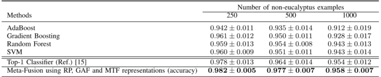
TABLE III
COMPARISON OF PERFORMANCE RESULTS,IN TERMS OF MEAN AND STANDARD DEVIATION OF BALANCED ACCURACY,AMONG THE BASELINE METHODS FOR FUSING CLASSIFIERS(FIRST FOUR ROWS),THE TOP-1CLASSIFIER THAT PRESENTED THE BEST RESULTS(PENULTIMATE ROW),AND THE
FUSION APPROACH ADOPTED FOR FUSING CLASSIFIERS(LAST ROW).
Number of non-eucalyptus examples
Methods 250 500 1000
AdaBoost 0.942 ± 0.011 0.935 ± 0.014 0.912 ± 0.019
Gradient Boosting 0.961 ± 0.012 0.950 ± 0.011 0.928 ± 0.017
Random Forest 0.959 ± 0.013 0.954 ± 0.008 0.943 ± 0.013
SVM 0.960 ± 0.009 0.951 ± 0.011 0.943 ± 0.014
Top-1 Classifier (Ref.) [15] 0.978 ± 0.013 0.964 ± 0.014 0.954 ± 0.012
Meta-Fusion using RP, GAF and MTF representations (accuracy) 0.982 ± 0.005 0.977 ± 0.007 0.958 ± 0.007
evaluated different approaches for fusion information available in the literature such as Bagging, Boosting, and Meta-fusion approaches: AdaBoost and Gradient Boosting are two fusion strategies that can be classified as Boosting approaches, while the Random Forest is a bagging approach by itself since several decision tree classifiers are training using the bagging approach. On the other, the Random Forest alongside with SVM algorithm can also be considered as a meta-fusion approach when they are used to have a second decision layer upon base classifiers.
Table III shows the performance results for the fusion methods investigated in this work. We could observe that baseline methods for fusion could not surpass the best result considering the individual performance of classifiers built in this work. On the other hand, the meta-fusion approach adopted in this work (see Section IV) achieved the best results, in terms of balanced accuracy, in comparison with the baseline methods for fusing classifiers.
Finally, it is important to notice that although our fusion approach needs to handle a high number of classification models in the training phase, the testing phase uses only the 60 classifiers selected during the training phase to produce the final decision. Of course, this number could be limited depend-ing on the efficiency aspects required by a target application. Remote sensing image classification is an active research field, and several real-time remote sensing applications have been addressed recently (e.g., applications that aim to predict natural disasters [44]). We believe that the investigation of the trade-off between effectiveness and efficiency of fusion approaches that handle a high number of pixelwise classification systems is an interesting research venue and could benefit applications that require fast decision-making with minimum latency.
VII. CONCLUSION
This paper addressed the pixelwise remote sensing im-age classification problem based on patterns found in time series associated with pixels. In particular, we investigated the complementary view provided by different classification systems created based on the combination of time series representations, data-driven feature extractors, and classifiers. Experiments were conducted aiming at addressing the problem of classifying eucalyptus plantations in remote sensing im-ages, based on vegetation index time series. Achieved results demonstrated that proposed ensemble exploits properly the
complementarity of different classification systems. In fact, state-of-the-art results were observed for the target dataset.
Future work focuses on improving our ensemble by exploit-ing the effectiveness of end-to-end classifiers based on data-driven learning approaches. We also plan to investigate the use of the proposed ensemble in spatiotemporal classification problems, and efficiency and yet effective strategies for build-ing multi-representational learnbuild-ing approaches that require fast decision-making with minimum latency.
REFERENCES
[1] N. Menini, A. E. Almeida, R. Lamparelli, G. L. Maire, R. Oliveira, J. Verbesselt, M. Hirota, and R. da S. Torres, “Tucum˜a: A toolbox for spatiotemporal remote sensing image analysis [software and data sets],” IEEE Geoscience and Remote Sensing Magazine, vol. 7, no. 3, pp. 110– 122, Sep. 2019.
[2] A. E. Almeida and R. da S. Torres, “Remote sensing image classifica-tion using genetic-programming-based time series similarity funcclassifica-tions,” IEEE Geoscience and Remote Sensing Letters, vol. 14, no. 9, pp. 1499– 1503, Sep. 2017.
[3] F. A. Faria, J. Almeida, B. Alberton, L. P. C. Morellato,
A. Rocha, and R. da Silva Torres, “Time series-based classifier fusion for fine-grained plant species recognition,” Pattern Recognition Letters, vol. 81, pp. 101–109, October 2016. [Online]. Available: http://www.sciencedirect.com/science/article/pii/S0167865515003670 [4] F. A. Faria, J. Almeida, B. Alberton, L. P. C. Morellato, and
R. da S. Torres, “Fusion of time series representations for plant recognition in phenology studies,” Pattern Recognition Letters, vol. 83, no. Part 2, pp. 205 – 214, November 2016. [Online]. Available: http://www.sciencedirect.com/science/article/pii/S016786551600074X [5] J. Almeida, J. A. dos Santos, B. Alberton, R. da S. Torres, and
L. P. C. Morellato, “Applying machine learning based on multiscale classifiers to detect remote phenology patterns in cerrado savanna trees,” Ecological Informatics, vol. 23, no. 0, pp. 49 – 61, 2014, special Issue on Multimedia in Ecology and Environment. [Online]. Available: http://www.sciencedirect.com/science/article/pii/S1574954113000654 [6] J. Almeida, D. C. G. Pedronette, B. C. Alberton, L. P. C.
Morellato, and R. da S. Torres, “Unsupervised distance learning for plant species identification,” IEEE Journal of Selected Topics
in Applied Earth Observations and Remote Sensing, vol. 9,
no. 12, pp. 5325–5338, December 2016. [Online]. Available:
http://ieeexplore.ieee.org/document/7590004/
[7] J. Almeida, J. A. dos Santos, B. Alberton, L. P. C. Morellato, and R. da Silva Torres, “Phenological visual rhythms: Compact representa-tions for fine-grained plant species identification,” Pattern Recognition Letters, vol. 81, pp. 90–100, October 2016. [Online]. Available: http://www.sciencedirect.com/science/article/pii/S0167865515004274 [8] V. Maus, G. Cˆamara, R. Cartaxo, A. Sanchez, F. M. Ramos, and
G. R. De Queiroz, “A time-weighted dynamic time warping method for land-use and land-cover mapping,” IEEE Journal of Selected Topics in Applied Earth Observations and Remote Sensing, vol. 9, no. 8, pp. 3729–3739, 2016.
[9] G. le Maire, S. Dupuy, Y. Nouvellon, R. A. Loos, and R. Hakamada, “Mapping short-rotation plantations at regional scale using MODIS time series: Case of eucalypt plantations in Brazil,” RSE, vol. 152, pp. 136– 149, Sep. 2014.
[10] A. J. Bagnall, J. Lines, A. Bostrom, J. Large, and E. J. Keogh, “The great time series classification bake off: a review and experimental evaluation of recent algorithmic advances,” Data Min. Knowl. Discov., vol. 31, no. 3, pp. 606–660, 2017. [Online]. Available: https://doi.org/10.1007/s10618-016-0483-9
[11] X. Wang, A. Mueen, H. Ding, G. Trajcevski, P. Scheuermann, and E. J. Keogh, “Experimental comparison of representation methods and distance measures for time series data,” Data Min. Knowl. Discov., vol. 26, no. 2, pp. 275–309, 2013. [Online]. Available: https://doi.org/10.1007/s10618-012-0250-5
[12] Z. Wang and T. Oates, “Imaging time-series to improve classification and imputation,” in Proceedings of the 24th International Conference on
Artificial Intelligence (IJCAI’2015). AAAI Press, 07 2015, pp. 3939–
3945.
[13] J. Eckmann, S. O. Kamphorst, D. Ruelle et al., “Recurrence plots of dynamical systems,” World Scientific Series on Nonlinear Science Series A, vol. 16, pp. 441–446, 1995.
[14] D. Dias, U. Dias, N. Menini, R. Lamparelli, G. L. Maire, and R. Torres, “Pixelwise remote sensing image classification based on recurrence plot deep features,” in IEEE International Geoscience and Remote Sensing Symposium, Yokohama, Japan, July 2019, pp. 1310–1313.
[15] D. Dias, U. Dias, N. Menini, R. Lamparelli, G. L. Maire, and R. da S Torres, “Image-based time series representations for pixelwise eucalyptus region classification: A comparative study,” IEEE Geoscience and Remote Sensing Letters, pp. 1–5, 2020.
[16] N. Menini, A. E. Almeida, R. A. C. Lamparelli, G. L. Maire, J. A. Santos, H. Pedrini, M. Hirota, and R. da S. Torres, “A soft computing framework for image classification based on recurrence plots,” IEEE Geoscience and Remote Sensing Letters, vol. 16, no. 2, pp. 320–324, Feb 2019.
[17] E. S. Santos, B. Alberton, L. P. Morellato, and R. da Silva Torres, “An information retrieval approach for large-scale time series retrieval,” in IEEE International Geoscience and Remote Sensing Symposium, Yokohama, Japan, July 2019, pp. 254–257.
[18] G. Huang, Z. Liu, L. Van Der Maaten, and K. Q. Weinberger, “Densely connected convolutional networks,” in Proceedings of the IEEE confer-ence on computer vision and pattern recognition (CVPR’2017), 07 2017, pp. 4700–4708.
[19] C. Szegedy, S. Ioffe, V. Vanhoucke, and A. A. Alemi, “Inception-v4, inception-resnet and the impact of residual connections on learning,” in Proceedings of the Thirty-First AAAI Conference on Artificial
Intelli-gence. AAAI Press, 02 2017, pp. 4278–4284.
[20] C. Szegedy, V. Vanhoucke, S. Ioffe, J. Shlens, and Z. Wojna, “Re-thinking the inception architecture for computer vision,” in Proceedings of the IEEE conference on computer vision and pattern recognition
(CVPR’2016). IEEE, 06 2016, pp. 2818–2826.
[21] A. G. Howard, M. Zhu, B. Chen, D. Kalenichenko, W. Wang, T. Weyand, M. Andreetto, and H. Adam, “Mobilenets: Efficient convo-lutional neural networks for mobile vision applications,” arXiv preprint arXiv:1704.04861, 04 2017.
[22] K. He, X. Zhang, S. Ren, and J. Sun, “Deep residual learning for image recognition,” in Proceedings of the IEEE conference on computer vision and pattern recognition (CVPR’2016), 06 2016, pp. 770–778. [23] K. Simonyan and A. Zisserman, “Very deep convolutional networks
for large-scale image recognition,” in Proceedings of the Interna-tional Conference on Learning Representations (ICLR’2015), vol. arXiv:1409.1556, 2014.
[24] F. Chollet, “Xception: Deep learning with depthwise separable convolu-tions,” in Proceedings of the IEEE conference on computer vision and pattern recognition (CVPR’2017), 07 2017, pp. 1251–1258.
[25] K. Wittkowski, “Classification and regression trees - l. breiman, j. h. friedman, r. a. olshen and c. j. stone.” Metrika, vol. 33, pp. 128–128, 1986. [Online]. Available: http://eudml.org/doc/176041
[26] K. H. Brodersen, C. S. Ong, K. E. Stephan, and J. M. Buhmann, “The balanced accuracy and its posterior distribution,” in 2010 20th
International Conference on Pattern Recognition. IEEE, 2010, pp.
3121–3124.
[27] J. Cohen, “A coefficient of agreement for nominal scales,” Educational and Psychological Measurement, vol. 20, no. 1, pp. 37–46, 1960. [Online]. Available: https://doi.org/10.1177/001316446002000104 [28] J. S. Iwanski and E. Bradley, “Recurrence plots of experimental data:
To embed or not to embed?” Chaos: An Interdisciplinary Journal of Nonlinear Science, vol. 8, no. 4, pp. 861–871, 1998.
[29] L. Ma, Y. Liu, X. Zhang, Y. Ye, G. Yin, and B. A. Johnson, “Deep learning in remote sensing applications: A meta-analysis and review,” ISPRS journal of photogrammetry and remote sensing, vol. 152, pp. 166–177, 2019.
[30] Q. Hu, D. Sulla-Menashe, B. Xu, H. Yin, H. Tang, P. Yang, and W. Wu, “A phenology-based spectral and temporal feature selection method for crop mapping from satellite time series,” International Journal of Applied Earth Observation and Geoinformation, vol. 80, pp. 218–229, 2019.
[31] H. Liu, F. Zhang, L. Zhang, Y. Lin, S. Wang, and Y. Xie, “Unvi-based time series for vegetation discrimination using separability analysis and random forest classification,” Remote Sensing, vol. 12, no. 3, p. 529, 2020.
[32] L. Zhang, S. Furumi, K. Muramatsu, N. Fujiwara, M. Daigo, and L. Zhang, “A new vegetation index based on the universal pattern de-composition method,” International Journal of Remote Sensing, vol. 28, no. 1, pp. 107–124, 2007.
[33] S. Feng, J. Zhao, T. Liu, H. Zhang, Z. Zhang, and X. Guo, “Crop type identification and mapping using machine learning algorithms and sentinel-2 time series data,” IEEE Journal of Selected Topics in Applied Earth Observations and Remote Sensing, vol. 12, no. 9, pp. 3295–3306, Sep. 2019.
[34] N. Rahimizadeh, S. B. Kafaky, M. R. Sahebi, and A. Mataji, “Forest structure parameter extraction using spot-7 satellite data by object-and pixel-based classification methods,” Environmental Monitoring object-and Assessment, vol. 192, no. 1, p. 43, 2020.
[35] B. Alberton, J. Almeida, R. Helm, R. da S. Torres, A. Menzel, and L. P. C. Morellato, “Using phenological cameras to track the green up in a cerrado savanna and its on-the-ground validation,” Ecological Informatics, vol. 19, no. 0, pp. 62 – 70, January 2014. [Online]. Available: http://www.sciencedirect.com/science/article/ pii/S1574954113001325
[36] B. Alberton, R. da S. Torres, L. F. Cancian, B. D. Borges, J. Almeida, G. C. Mariano, J. dos Santos, and L. P. C. Morellato, “Introducing digital cameras to monitor plant phenology in the tropics: applications for conservation,” Perspectives in Ecology and Conservation, vol. 15, no. 2, pp. 82 – 90, Apr. 2017. [Online]. Available: http://www.sciencedirect.com/science/article/pii/S2530064417300019 [37] J. Almeida, J. A. dos Santos, W. O. Miranda, B. Alberton,
L. P. C. Morellato, and R. da S. Torres, “Deriving vegetation indices for phenology analysis using genetic programming,” Ecological Informatics, vol. 26, Part 3, pp. 61 – 69, 2015. [Online]. Available: http://www.sciencedirect.com/science/article/pii/S1574954115000114 [38] F. A. Faria, J. A. dos Santos, A. Rocha, and R. da S. Torres,
“A framework for selection and fusion of pattern classifiers in multimedia recognition,” Pattern Recognition Letters, vol. 39, no. 0, pp. 52 – 64, April 2014, advances in Pattern Recognition and Computer Vision. [Online]. Available: http://www.sciencedirect.com/ science/article/pii/S0167865513002870
[39] A. Kuehlkamp, A. Pinto, A. Rocha, K. W. Bowyer, and A. Czajka, “Ensemble of multi-view learning classifiers for cross-domain iris pre-sentation attack detection,” IEEE Transactions on Information Forensics and Security, vol. 14, no. 6, pp. 1419–1431, 2018.
[40] J. R. Landis and G. G. Koch, “The measurement of observer agreement for categorical data,” Biometrics, vol. 33, no. 1, 1977.
[41] Y. Freund and R. E. Schapire, “A decision-theoretic generalization of on-line learning and an application to boosting,” J. Comput. Syst. Sci., vol. 55, no. 1, p. 119–139, Aug. 1997. [Online]. Available: https://doi.org/10.1006/jcss.1997.1504
[42] C. M. Bishop, Pattern Recognition and Machine Learning (Information
Science and Statistics). Berlin, Heidelberg: Springer-Verlag, 2006.
[43] J. H. Friedman, “Greedy function approximation: A gradient boosting machine,” The Annals of Statistics, vol. 29, no. 5, pp. 1189–1232, 2001. [44] K. Nogueira, S. G. Fadel, I. C. Dourado, R. de O. Werneck, J. A. V. Mu˜noz, O. A. B. Penatti, R. T. Calumby, L. T. Li, J. A. dos Santos, and R. da Silva Torres, “Exploiting convnet diversity for flooding identification,” IEEE Geoscience and Remote Sensing Letters, vol. 15, no. 9, pp. 1446–1450, Sept 2018.
Danielle Dias received the B.Sc. degree in computer science from the Federal University of Par´a (UFPA), Brazil, in 2005, the M.Sc. degree in Computational Modelling from the Federal University of Alagoas (UFAL), Brazil, in 2008, and the Ph.D. degree in computer science from the University of Campinas (Unicamp), Brazil, in 2020. Her research interest is in the area of machine learning applied to remote sensing.
Allan Pinto is a Postdoctoral Researcher at the University of Campinas (Unicamp), Brazil. He re-ceived a B.Sc. degree in Computer Science from the University of S˜ao Paulo (USP), Brazil, in 2011, an M.Sc. in Computer Science from the University of Campinas (Unicamp), Brazil, in 2013, and a Ph.D. degree in Computer Science at the same university, in 2018. A part of his doctoral was accomplished at the University of Notre Dame, USA, in which he worked on different topics such as Presentation Attack Detection in Biometric Systems, Content-based Image Retrieval, and Multimedia Forensics. Currently, he is a member of the editorial board of the Forensic Science International: Reports. He is also a member of the IEEE.
Ulisses Dias received the B.Sc. degree in computer science from the Federal University of Par´a (UFPA), Brazil, in 2005, the M.Sc. degree in Computational Modelling from the Federal University of Alagoas (UFAL), Brazil, in 2007, and the Ph.D. degree in computer science from the University of Campinas (Unicamp), Brazil, in 2012. He is an assistant pro-fessor with the School of Techonology, Unicamp. Brazil.
Rubens Lamparelli received his Ph.D. degree in Transport Engineering from University of S˜ao Paulo, Brazil, 1998. He is currently a researcher at NIPE (Interdisciplinary Center on Energy Planning), as Agricultural Engineer, specialized in Remote Sens-ing and GeoprocessSens-ing. His researchers explore is-sues like Environmental, Agricultural and Energy and their interactions.
Guerric Le Maire works on remote sensing of forest, in close relation with carbon and water budget modelling. His works concern the classification and estimation of forest characteristics from satellite im-ages, such as leaf area index, chlorophyll content or biomass, with many applications on eucalypt plan-tations. Guerric has a diploma from AgroParisTech (French Higher Educational Institution), a M.Sc. in Ecology, a Ph.D. in Ecophysiology. He is re-searcher at CIRAD (Eco&Sols Joint unit, Montpel-lier, France), and is currently Visiting Professor at UNICAMP (University of Campinas, Brazil) where he develops projects related with monitoring of eucalypt plantations at regional scale. He has published more than 60 papers in the field of remote sensing or process-based forest modelling.
Ricardo da S. Torres is Professor in Visual Com-puting at the Norwegian University of Science and Technology (NTNU). He used to hold a position as a Professor at the University of Campinas, Brazil (2005 - 2019). Dr. Torres received a B.Sc. in Com-puter Engineering from the University of Campinas, Brazil, in 2000 and his Ph.D. degree in Computer Science at the same university in 2004. Dr. Tor-res has been developing multidisciplinary eScience research projects involving Multimedia Analysis, Multimedia Retrieval, Machine Learning, Databases, Information Visualisation, and Digital Libraries. Dr. Torres is author/co-author of more than 200 articles in refereed journals and conferences and serves as a PC member for several international and national conferences. Currently, he has been serving as Senior Associate Editor of the IEEE Signal Processing Letters and Associate Editor of the Pattern Recognition Letters. He is a member of the IEEE.