ACEt: An R Package for Estimating Dynamic Heritability and Comparing Twin Models

ACEt: An R Package for Estimating Dynamic

Heritability and Comparing Twin Models

Citation He, Liang, et al. “ACEt: An R Package for Estimating Dynamic

Heritability and Comparing Twin Models.” Behavior Genetics, vol. 47, no. 6, Nov. 2017, pp. 620–41.

As Published http://dx.doi.org/10.1007/s10519-017-9866-y

Publisher Springer US

Version Author's final manuscript

Citable link http://hdl.handle.net/1721.1/113827

Terms of Use Article is made available in accordance with the publisher's

policy and may be subject to US copyright law. Please refer to the publisher's site for terms of use.

ACEt: an R package for estimating

dynamic heritability and comparing twin

models

Liang He1,2*, Janne Pitkäniemi3,4, Karri Silventoinen3,5, and Mikko J. Sillanpää6,7 Running title: R package estimating dynamic heritability

1

Broad Institute of MIT and Harvard, Cambridge, Massachusetts, USA

2

Computer Science and Artificial Intelligence Laboratory, MIT, Cambridge, Massachusetts, USA

3

Department of Public Health, University of Helsinki, Finland,

4

Finnish Cancer Registry, Institute for Statistical and Epidemiological Cancer Research, Helsinki, Finland,

5

Population Research Unit, Department of Social Research, University of Helsinki, Helsinki, Finland,

6

Department of Mathematical Sciences, University of Oulu, Finland,

7

Biocenter Oulu, University of Oulu, Finland.

* Corresponding authors: Liang He Email: lianghe@mit.edu

Abstract

Estimating dynamic effects of age on the genetic and environmental variance components in twin studies may contribute to the investigation of gene-environment interactions, and may provide more insights into more accurate and powerful estimation of heritability. Existing parametric models for estimating dynamic variance components suffer from various drawbacks such as limitation of predefined functions. We present ACEt, an R package for fast estimating dynamic variance components

and heritability that may change with respect to age or other moderators. Building on the twin models based on penalized splines, ACEt provides a unified framework to incorporate a class of ACE models, in which each component can be modeled independently and is not limited by a linear or quadratic function. We demonstrate that ACEt is robust against misspecification of the number of spline knots, and offers a refined resolution of dynamic behavior of the genetic and environmental components and thus a detailed estimation of age-specific heritability. Moreover, we develop resampling methods for testing twin models with different variance functions including splines, log-linearity and constancy, which can be easily employed to verify various model assumptions. We evaluated the type I error rate and statistical power of the proposed hypothesis testing methods under various scenarios using simulated datasets. Potential numerical issues and computational cost were also assessed through simulations. We applied the ACEt package to a Finnish twin cohort to investigate age-specific heritability of body mass index and height. Our results show that the age-specific variance components of these two traits exhibited substantially different patterns despite of comparable estimates of heritability. In summary, the ACEt R package offers a useful tool for the exploration of age-dependent heritability and model comparison in twin studies.

Key words: twin model comparison, dynamic heritability, penalized splines, likelihood ratio test, ACEt

Introduction

Twin studies offer unique advantages to examine the overall impact of genes and environment on a phenotype, and hence are broadly employed in estimating heritability for many complex traits (Polderman et al. 2015). The influence of genes and environment on a specific quantitative trait, such as body mass index (BMI) may be dependent on age or other moderators (Réale et al. 1999; Jelenkovic et al. 2015). This age-dependent phenomenon has also been observed in behavioral genetics research. For example, the correlation in twins on cannabis use is higher when they are measured at the age of 18 than 16 (Distel et al. 2011). Refined estimation from twin studies of how genetic and environmental components evolve with respect to age may contribute to the exploration of gene-environmental interactions and may help elucidate the gap of estimated heritability between twin studies and genome-wide

association studies (GWAS). For example, the potential missing heritability (Eichler et al. 2010) may partly attribute to effects from epigenetic markers that are not captured by general GWAS but are reflected in the estimation of twin studies. In addition, given age-specific heritability, a sample at the age when the heritability peaks can be chosen for GWAS to achieve the largest statistical power.

Recent evidence suggests the important role of examining dynamic component variance; however, the existing twin models for this problem assuming a linear or quadratic form of the moderator effects (Purcell 2002) are often too restricted in reality. Moreover, the incorrect model assumptions would result in dramatically biased estimates and misleading interpretation

(He et al. 2016). So far, very little attention has been paid to the estimation of dynamic heritability without a prior knowledge of its functional form, i.e., whether the genetic and environmental variance components change as a function of age or environmental exposure. Recently, (Briley et al. 2015) proposed a nonparametric method based on local structural equation modeling (LOSEM) to estimate the dynamics of variance components, which does not require a pre-specified functional form. Despite of its flexibility in model specification, this nonparametric method is sensitive to the choice of certain parameters related to a kernel function for weighting observations and is not straightforward for model comparison. In addition, (He et al. 2016) have proposed two semiparametric models, in which the ACE(t)-p model (throughout the article we use ACE(t)-p as the abbreviation) is less dependent on user-defined parameters requiring prior knowledge of the component variance functions. These models allow dynamic additive genetic (A) and common environmental (C) components and a constant unique environmental (E) component (He et al. 2016). Unlike most methods based on the SEM framework (Rijsdijk and Sham 2002), these models treat variance components (A, C, E) as random effects in a linear model (as discussed in (Visscher et al. 2004)), and furthermore, the variance of the components is modeled as a function of age. The basic idea is to directly estimate the variance functions using B- or penalized B-splines (P-splines) (Eilers and Marx 1996) rather than assuming them to be constants as in the classical ACE model (Zyphur et al.

2013) or a known functional form. B-splines (De Boor 1978) constructed piecewisely from polynomial functions are an appealing methods for the nonparametric function estimation. Similar to locally weighted scatterplot smoothing (LOWESS) (Cleveland 1979) in some sense, it has the overfitting problem if excessive B-spline basis functions are used (i.e., too many parameters). Nevertheless, we can smooth adjacent spline coefficients to be more alike to reduce the dimension of the curve parameters. P-splines tackle the overfitting problem by introducing a penalizing coefficient to smooth the coefficients of the B-spline basis functions (Eilers and Marx 1996). In ACE(t)-p, the penalizing coefficients for smoothing the B-spline coefficients are first estimated by an empirical Bayes method before used for estimating the variance curves for the components. A simple Markov chain Monte Carlo (MCMC) method is proposed for estimating the pointwise confidence intervals (CIs) for the estimated variance curves. The performance of the estimation procedure has been evaluated through a simulation study and its utility has been demonstrated through an application to a Finnish twin study for discovering the temporal patterns of genetic and environmental variance curves of BMI (He et al. 2016).

In this work, we introduce the R package ACEt which further generalizes the previous models

(He et al. 2016), and provides functions that facilitate model comparisons between twin models of different variance functional forms. First, we describe a unified framework in which the A, C and E variance components can be independently modeled by spline, log-linear or constant functions (including zero which corresponds to the elimination of a component). We show that this unified framework incorporates the classical ACE, AE and CE models as special cases. We assess the estimation accuracy and performance through simulation studies under various settings. In addition, we implement a function to estimate the dynamic heritability, the definition of which is given in the Methods section, together with its pointwise CIs based on the estimated variance curves. Once we show that these models with different components and functions can be fitted under a single framework, it is natural to ask which variance function is the best fitting for a given dataset or how to select a better model. For example, in some cases,

it is desirable to test the linearity of a C component to see whether there is an accumulative environmental effect. Answering this sort of questions requires methods for comparing parametric and semiparametric models. In contrast to the LOSEM proposed by (Briley et al. 2015), it is straightforward and fast to draw inference under the spline-based framework by, for example, leveraging likelihood ratio tests (LRTs) (Ruppert et al. 2003; Crainiceanu and Ruppert 2004). We show in this work how the hypothesis testing for model selection can be addressed separately using different strategies for the ACE(t) and ACE(t)-p models which employ B-splines and P-splines, respectively. We perform detailed simulation studies under various settings to examine the type I error rate, statistical power and other potential numerical issues. We then investigate the dynamic heritability of BMI and height with a Finnish twin cohort, finding that they follow substantially different temporal patterns.

The rest of the paper is organized as follows. In the Methods section, we first specify the generalized ACE(t) and ACE(t)-p models and briefly review the proposed estimation procedure. Then, we elaborately describe how hypothesis testing can be conducted using different strategies for the ACE(t) and ACE(t)-p models, during which more emphasis is placed on how to test constancy and log-linearity in ACE(t)-p. We define the dynamic heritability and provide a derivation for estimating the dynamic heritability and obtaining its CIs using a delta method. At the end of this section, we give an introduction to the functions provided in the R package ACEt and illustrate a practical application to an example dataset in a vignette. In the Results section, we assess the performance of the estimation of the variance components and the proposed hypothesis testing methods for model comparison through simulated datasets. Influence of some practical numerical issues will also be examined. As a demonstration of its utility in real data analysis, we investigate the dynamic heritability of BMI and height with a Finnish twin cohort. The results and future extension are summarized in the Discussion section.

Methods

Model Specification and Estimation Procedure

In the classical ACE twin model, the variance of a phenotype is decomposed into the additive genetic component , the shared environmental component and the unique environmental component . Instead of being constants, now assuming that the three components are functions of a variable of interest such as age, we are interested in estimating the variance functions , and . Suppose that there is no prior knowledge of the functional form, a natural approach can be to represent the functions using a set of independent basis functions (e.g., power series, Fourier series) that can approximate the functions arbitrarily well by taking a linear combination of a sufficiently large number K of these basis functions. For example, a quadratic polynomial can be written as a linear combination of the basis functions , , and with the coefficients . A class of commonly used basis functions is B-spline functions. To approximate an unknown function using B-splines, the interval of the estimated function is divided into subintervals by a group of interior knots, and over each subinterval a spline is defined as a polynomial function of a given degree , (i.e., the highest power) (De Boor 1978; Ramsay and Silverman 2005). The kth B-spline basis function of the degree is defined recursively as

,

.

The ACE(t) model (throughout the article we use ACE(t) as the abbreviation) proposed by (He et al. 2016) employ B-splines with (De Boor 1978) for estimating the variance functions of the A and C components under the assumption of a constant E component. We now relax this assumption and allow all components to be independently modeled by different functions of . The total variance of a quantitative trait, which is defined as the conditional variance

calculated at , can be decomposed into the A, C and E components. Let us denote by , and the variance functions for the A, C and E components, respectively. We then represent each variance function separately using an exponential of a linear combination of B-splines (De Boor 1978)

(1)

where is a vector of the B-spline basis functions for the component evaluated at and is a vector of the corresponding spline coefficients. is the number of spline coefficients (i.e., the number of interior knots minus one plus the degree of B-splines , which is set at 2 in the current implementation). The exponential is to ensure that the variance is non-negative, which is also proposed in (Turkheimer and Horn 2014). The knots can be evenly distributed or be placed based on the quantiles of the sample. In our implementation, we leave the number of knots defined by users. It can be seen from (1) that it simplifies to the classical ACE model (Zyphur et al. 2013) when satisfies for each component because in this case we have

which is independent of . One practical issue of B-splines is that its performance is sensitive to the choice of the number of knots (illustrated in the Results section), and excessive knots would lead to overfitting the data. Thus, ACE(t)-p uses P-splines (which stands for “penalized B-spline”) (O’Sullivan 1986; Eilers and Marx 1996) that are defined on evenly distributed knots and introduce a difference penalty to control the smoothness of , so that it can address the overfitting problem (More information about the difference penalty can be found in e.g., (Wood 2006)). Specifically, the penalization for overfitting is achieved by introducing a multivariate normal prior assigned on the spline coefficients of each component. More details of the ACE(t)-p model are given in Appendix A.

The estimation strategy follows the similar spirit of that described previously (He et al. 2016) with some extensions. Specifically, spectral decomposition is employed in order to test log-linearity which is described in the following subsection. It also improves the performance of the MCMC sampling in constructing CIs by avoiding strong posterior correlation between spline coefficients when they are almost linear. Following the same notation in (He et al. 2016), suppose that we have zero-mean normally distributed quantitative phenotypic data (an vector) and (an vector) for monozygotic (MZ) and dizygotic (DZ) twin pairs. Note that if the initial phenotypic data are not zero-mean, we can always centralize them, for example, by fitting a linear regression model and using residuals as the input. We also have the information of age at which and are measured, denoted by (an vector) and (an vector) for the MZ and DZ twins. In fact, age can be replaced by any other quantitative moderator of interest of which we intend to investigate the dynamic effects on the variance components as long as it is measured at the twin level (e.g., birth year). This is also called measures of the shared environment (Turkheimer et al. 2005).

Based on the general assumption in the ACE twin model (i.e., MZ and DZ twins share 100% and 50% of the A component, respectively, and 100% of the C component.), the covariance matrices of and are

_,

_,

where , , , denotes the Kronecker product and converts a vector to a diagonal matrix with the vector entries as its diagonal elements. Thus, provided that there is no between-pair correlation among the twins, the phenotype vector follows a zero-mean multivariate normal distribution,

To estimate the spline coefficients , where the prime represents transpose, the maximum likelihood estimation (MLE) finds the solutions that maximize the following log-likelihood, i.e.,

_.

As it is difficult to express the solutions analytically, numerical algorithms such as the Newton’s method are needed to find . The Newton's method requires further calculating the second derivative of the likelihood, so we instead employ the L-BFGS algorithm (Byrd et al. 1995) which is computationally faster (e.g., implemented in the 'optim' R function). The L-BFGS algorithm is a fast Quasi-Newton algorithm that does not involve calculating the Hessian matrix analytically. The performance of the approximation of the Hessian matrix by the L-BFGS algorithm is assessed in the Results section. The variance of the estimates and thus the pointwise CIs of the estimated variance curves can be obtained by either a delta method based on the asymptotic normal consistency of MLE or a bootstrap method. The delta method provides a first order approximation for the distribution of a function of MLE by utilizing Taylor’s theorem. The two methods have comparable results in general (He et al. 2016); however, we find in our simulation study that despite the high computational intensity, the bootstrap method is more robust when the true values of the spline coefficients are on their boundary in which case the normality of the MLE does not hold. The estimation algorithm in this extended ACE(t)-p model is similar to that in (He et al. 2016). Spectral decomposition of the penalty matrix is adopted in the MCMC method for estimating the CIs. More details are given in Appendix A.

Note that it is possible to incorporate a mean function under a unified framework with the variance components. One of the major benefits of including the mean function is that we can pursue an unbiased estimate of the variance components by instead using the restricted maximum likelihood (REML) that accounts for the loss in degrees of freedom for estimating the parameters in the mean. The REML estimation provides more accurate estimates if the number

of the covariates in the mean function is large or even comparable to the sample size (Harville 1977). In the current implementation, however, we do not include the mean function in the estimation procedure to diminish the computational burden especially in ACE(t)-p where resampling methods are used for model comparisons as discussed later. Fortunately, twin studies typically require large sample size, and thus the gain from REML is very limited. Therefore, the phenotype should be centered before treated as an input. For example, the residuals from a regression model in which an appropriate mean function is specified can be used. The dynamic variance components and heritability considered in this study are age-specific, which means that the variance is computed conditionally at each age (i.e.,

). It should be noted that here we are interested in the modulating effect of age on the shared environmental variance component, that is, how age affects the contribution of other shared-environmental factors to the C component. If age is a major shared-environmental measurement per se, it should be included in and be properly regressed, so that its modulating but not direct effect is reflected in ; otherwise, the estimate for the modulating effect would be inflated or incorrectly estimated. Let us consider a situation where the age of a sample has a normal distribution and has a linear effect on the phenotype (i.e., ). It follows for a DZ twin pair of the age that

.

If we omit age from , the contribution of age to the shared-environmental variance would be included in the estimate of the C component, which would be

Hypothesis testing for comparison of Twin Models

In many cases, it is useful to model some components with splines and others with a constant that can be zero. For example, we show in a following real data analysis that two components of height are almost constant after some age, and thus, modeling them with constants can reduce the estimation uncertainty. When fitting a given twin dataset using more complex models, it may also be of primary concern to select the best twin model by comparison. In the case of ACE(t), it is straightforward to test a constant or log-linear component by using the LRT as they are nested models of the spline model. A constant variance for component is equivalent to a spline model with homogeneous spline coefficients, i.e., . In the log-linear case, we have when the knots are evenly distributed. It is noted that the correct distribution should be used when testing the variance component in the twin models (Visscher 2006). In general cases, when the constancy of the tested component is true, the LRT statistic asymptotically follows a distribution with ( in the log-linear case) degrees of freedom according to Wilks' theorem (Wilks 1938) provided that the true variance functions of the other components belong to the functional space spanned by the basis functions. If the variance functions of the other components are misspecified or are not in the functional space spanned by the basis functions, the LRT test does not work properly. In a special case, testing a zero variance component corresponds to testing the null hypothesis of , which lies in the boundary of the parameter space. The asymptotic distribution of this LRT statistic under such non-regular conditions has been investigated under various scenarios (Chernoff 1954; Self and Liang 1987). Under a unified framework, it has been shown that the LRT statistic follows a (chi-bar-square) distribution when some regularity conditions hold (Shapiro 1988). For a simple situation where there is only one variance component of interest and the true values of the parameters for the other components are not on the boundary of the parameter space, the LRT statistic for comparing a zero component (the null hypothesis) and a constant component asymptotically follows a mixture of two distributions with and degree of freedom (this is the case 5 in (Self and Liang 1987)). Our simulation results (not shown here) confirm that the empirical distribution

of the LRT statistic in the above situation is in accordance with its theoretical asymptotic distribution under the null hypothesis. More complicated situations are discussed in details by (Dominicus et al. 2006). Alternatively, simulation-based methods can be employed to acquire the empirical null distribution of the statistic numerically in the case of more complex models.

Unlike ACE(t), testing constancy or linearity in ACE(t)-p is more complicated. Testing the log-linearity of a component in ACE(t)-p is equivalent to testing the following hypothesis,

.

If the LRT is used, the major challenge is to obtain the null distribution because the asymptotic distribution (a mixture of two distributions) is not valid in this case (Ruppert et al. 2003). We thus propose a parametric bootstrap method which is shown to work properly in the simulation study. Detailed information of the method is given in Appendix B.

Testing the constancy against log-linearity is relatively straightforward in ACE(t)-p. The inference can be made based on the estimated coefficients and their variance estimated from the MCMC method. One problem to be solved is that the variance obtained in the previous work (He et al. 2016) is underestimated because it does not take into account the uncertainty of for the other spline components. We propose a resampling method to correct for the underestimation of the variance, and provide a detailed description of the method for testing constancy in Appendix C.

Estimation of Dynamic Heritability

Other than the absolute values of variance, we are interested in the proportion of age-specific variation that is explained by the A, C and E components, respectively. In particular, the heritability, which is the proportion of the total variance attributed to the genetic differences

between individuals, is an important concept in quantitative genetics. Given the estimates of the dynamic variance components, we are ready to further estimate the dynamic heritability curve. We define the age-specific (or other moderators) heritability for the ACE model as

.

The following derivation is based on the ACE model, and if the AE model is adopted, in the denominator of the right-hand side is eliminated. By substituting with (1), the estimated dynamic heritability follows

, (3)

where is a vector of the B-spline basis functions evaluated at . The variance of the estimated heritability at can be obtained either from a delta method or a bootstrap method. Denote by the estimated spline coefficients from either ACE(t) or ACE(t)-p, and by the covariance matrix of , which is estimated from the MLE in the case of the ACE(t) model and from the posterior distribution in the case of ACE(t)-p. We notice that the estimated heritability equals

, where .

As and are affine transformations of , we have

.

By applying the delta method and substituting with its estimate , it follows that .

The CI at can be calculated based on the assumption of an approximately normal distribution of . On the other hand, the pointwise variance of the estimated dynamic heritability

can also be acquired from a parametric bootstrap method described previously (He et al. 2016). In the bootstrap method, each bootstrap estimates of the heritability at is calculated according to the equation (3) from a bootstrap replicate sampled from the formula (2) with plugged in. The delta method may not be accurate when the estimated heritability or component variance approaches its boundary. In this situation, the bootstrap method is recommended.

Software overview

To use the ACEt R package, the data set should be prepared in a matrix format for MZ and DZ twins separately in which each row for a twin pair contains three columns (the first two are phenotypes and the third is age or other moderators of interest). An example data set is given in the package, and an example of its application is described in the supplementary materials (Text S1). The phenotypic data should be zero-mean normally distributed and preferably adjusted by age as aforementioned. The AtCtEt function estimates variance curves using B-splines in which users can specify whether the variance of each component is dynamic, constant or zero. Users need to provide the number of knots and how the knots are distributed, evenly or quantile-based. Our previous simulation shows that the pointwise CIs computed from the Hessian matrix provided by the maximum likelihood estimation are comparable to those from the bootstrap method, but when the curves are close to their boundaries the bootstrap method is recommended. The AtCtEtp function corresponds to ACE(t)-p in which users can specify a component to be modeled by splines, a linear function or a constant. The acetp_mcmc function implementing an MCMC method is dedicated to producing the empirical Bayes estimates and to generating the covariance matrix for the estimates. Two model comparison methods for ACE(t)-p are provided by the test_acetp function. Finally, variance curves and dynamic heritability with their pointwise CIs can be plotted using the plot_acet function either with the delta or the bootstrap method.

Results

In this section, we evaluate the performance of the proposed models in estimating the variance components and testing twin models. More specifically, we first assess the accuracy of the estimation in terms of average mean square errors (AMSEs). The type I error rate and the empirical power of the testing procedures are then evaluated by simulations. We then report a rough estimate of the computational cost of the estimation algorithm in ACE(t) and ACE(t)-p. Finally, as a demonstration of the proposed package, we analyze the dynamic heritability of BMI and height for a Finnish twin cohort. The sample sizes of the MZ and DZ twins in all of the following simulation studies are set to be equal although there are often more DZ twins than MZ twins in twin studies. In the Appendix, we further discuss the robustness of the estimation algorithm against the selection of the initial values (Appendix D), and compare different methods (analytical Hessian vs. approximate Hessian, bootstrapping vs. delta method) for estimating the CIs (Appendix E and F).

Evaluation of the accuracy of the estimation

To evaluate how many samples are needed to obtain accurate estimates of the variance functions, we compute the following AMSE for component based on points evenly placed across the age interval,

, (4) where we chose , which is sufficient to produce a reliable estimate of AMSE for the smooth functions assessed in the following simulation study. The same AMSE has previously been used to assess the performance of the models in which only two components are set to be dynamic (He et al. 2016). In this simulation, we were interested in further figuring out whether more samples would be needed to achieve the same AMSEs if the number of dynamic components increased up to three. We also assessed the possible impact of the initial values on

the estimation procedure. To simplify the comparison, we used the same quadratic and power functions for the A and C components as in (He et al. 2016),

,

_,

and additionally the following oscillation function for the E component,

.

A plot of the three variance functions is given in the supplementary materials (Figure S1). We evaluated the AMSEs under scenarios of different numbers of interior knots, twin pairs and initial values. In each scenario, the estimated AMSEs were computed using the equation (4) from 100 simulated datasets based on the above twin model with sampled from a uniform distribution .

In the case of ACE(t), we observed that the AMSEs for the three components dropped substantially with the number of twin pairs increasing from 5,000 to 20,000 in all scenarios (Figure 1). The AMSEs for the E component were much lower than those for the A and C components. The AMSEs rose rapidly for the A and C components with the number of interior knots increasing from 5 to 12, but decreased for the E component. With the same sample sizes, the estimated AMSEs for the A and C components were comparable to the estimates from the previous simulation study in which the E component had a constant variance (Table 2 in (He et al. 2016)), suggesting that increasing the number of dynamic components did not require more samples to attain the same AMSE. The results also showed that trying additional randomly generated initial values had little impact on the AMSEs.

Akin to the trend observed for ACE(t), the results for ACE(t)-p showed that the AMSEs dropped rapidly with the increasing twin pairs, particularly from 5,000 to 10,000 (Figure 2). The results

also indicated that using multiple initial values at the suggested magnitude (See supplementary materials D) had little influence. However, we observed different patterns with respect to the number of knots. Specifically, the AMSEs for the E component decreased with the knots increasing from 8 to 20, which were similar to that from ACE(t), while the AMSEs rose very modestly with the increasing knots for the A component and there was almost no evident upward trend for the C component, indicating that the performance of ACE(t)-p was robust against excessive knots. Comparing with the results from ACE(t), we found that the AMSEs for ACE(t)-p were substantially lower under the same settings.

Evaluation of type I error rate

First, we check that the proposed parametric bootstrap method for testing log-linearity of a component variance in ACE(t)-p works properly under different settings. In each setting, we simulated a phenotypic dataset of 10,000 twin pairs. We examined the null distribution of the p-values for testing a log-linear C component. In principle, the choice of the C component is arbitrary because the bootstrap method for LRT does not require a specific component. However, as found in the previous subsection, the estimation for the A and C components is more prone to error than the E component. Therefore, we are more interested in checking the type I error rate for the A or C component. In the first case, we assumed a log-linear C component and kept the A and E components as constants ( ). We also examined the null distribution under different numbers of initial values attempted in the EM algorithm. The Q-Q plot of the p-values (Figure 3) showed that there was a slight deviation from the expected null distribution only in the case of one initial value, suggesting that using multiple initial values had a modest benefit to control type I error rate. Nevertheless, computational cost grows linearly with the initial value attempts, which can become a major burden for the intensive bootstrap procedure. In the second case, we replaced the constant function of the A component by splines to examine whether the performance was affected by the existence of another spline term. The spline coefficients for the A component were randomly generated from a zero-mean normal

distribution with . We used 8, 10 and 12 interior knots to test the sensitivity to the number of knots in the spline term. Our simulation results showed that the distribution of the p-values under the null hypothesis obtained by the bootstrap method was not affected by the existence of another spline term other than the tested component or the number of the knots in the spline term under the null model (Figure 4). Again, the deviations from the expected null distributions in the case of one initial value were trivial in these scenarios.

To evaluate the proposed correction method for testing constancy in ACE(t)-p, we still checked Q-Q plots to compare the null distributions of the p-values before and after the variance correction. We tested a constant versus a log-linear E component under the same simulation setting as the above second case. We chose , the number of resampling used for the variance correction (see Appendix C for more details). Our simulation results showed that there was a modest inflation of the type I error rate without the correction and the inflation disappeared after applying this correction (Figure 5). Similarly, the empirical type I error rate was well controlled for testing the A or C component when the tested component was comparable to the other components (the results not present here). However, when the A or C component was much smaller than the E component, we observed inflation of type I error rate.

Evaluation of statistical power

We assessed empirical statistical power of the proposed testing methods for the ACE(t) and ACE(t)-p models through simulated datasets. We focused on providing a rough estimate of the sample size needed for detecting a small deviation from the null hypothesis in each proposed test. We also examined the extent to which the statistical power was affected by other factors such as the ratio of the tested variance to the total variance. We assumed a twin model with a spline A component , a constant C component and a log-linear E component . The simulation setting was chosen to mimic the variance functions and the similar scale of BMI in the previous Finnish twin study (He et al. 2016). For the ACE(t)

model, we considered two sorts of tests: (1) zero against constancy of the C component, and (2) constancy against linearity of the E component. For ACE(t)-p, we considered the following tests: (2) constancy against linearity of the E component and (3) linearity against non-linearity of the A component. The rationale of choosing these tests is that we are more interested in testing a zero C component as the previous results on BMI show that the C component almost disappear after some age (He et al. 2016). Testing a constant E component is also of importance because a linearly increasing E component indicates that the phenotype is subject to accumulative environmental effect as we will see in the following real data analysis. Additionally, testing non-linearity of the A component may give us some information about gene-environmental interaction. For (1), we evaluated the empirical power by first changing the variance of the C component between 0.1 and 0.3 with , and fixed. To further assess whether the power was affected by the total variance, we then tuned between log(4) and log(12) given . For (2), we evaluated the empirical power by first changing the slope between 0.0025 and 0.01 with , and fixed. We then assessed whether the power was affected by the intercept and the total variance, we changed between 4 and 12 and between 1.5 and 2.5. For (3), we changed the variance for the spline coefficients of the A component between 0.01 and 0.1 ( corresponding to linearity) with , and fixed. In each test, we calculated the empirical power from 200 simulated twin datasets and evaluated the power under different sample sizes ranging from 6,000 to 12,000 twin pairs (50% MZ and 50% DZ twins). The age of each twin pair was randomly generated from a uniform distribution .

We observed that at least 12,000 twin pairs were needed to yield a power larger than 0.8 for detecting the existence of in ACE(t) when the total average variance was ~4.5 (Figure 6A). The statistical power dropped dramatically with the increasing total variance. As shown in Figure 6B, even with 12,000 twin pairs the power was smaller than 0.5 when the total average variance became ~6.5, and was almost imperceptible when it was ~14.5. The results from the

tests for constancy in ACE(t) show that 10,000 twin pairs were necessary to yield a statistical power of 80% for detecting a linear variance increasing with age from 1 to 1.25 (corresponding to ) given the total average variance of ~6 (Figure 6C). Unlike the test for existence, the power of LRT for detecting non-constancy was mildly affected by the total variance (Figure 6D) and the intercept (Figure 6E).

Comparison between Figure 6C and 7A suggested that the test for constancy in ACE(t)-p was somewhat more powerful than that in ACE(t) when the true variance function is linear. This is expected as the alternative model is linear when testing a constant component in ACE(t)-p. At least 6000 twin pairs were required for a power of 80% when detecting . The results (Figure 7B) showed that a large sample size (>12,000 twin pairs) was necessary to achieve a power of 80% for detecting .

Evaluation of computational cost

The current implementation of the models makes it feasible to estimate dynamic variance components for large-scale twin data sets within a few seconds, especially in the case of ACE(t). We considered the factors including sample size, the function form (i.e. spline, log-linear or constant) of a variance component, the number of knots to investigate the computational cost. It should be noted that a specific dataset and the number of parameters also determine the speed of convergence of the L-BFGS algorithm. Table 1 gives rough estimates of the average computational time of ACE(t) and ACE(t)-p based on three randomly generated simulation datasets. The estimation was conducted on an Intel i7-4790, 16G RAM PC. It seemed that the computational time grew almost linearly with sample size in ACE(t). We also observed that when the number of knots was large (e.g. >10), the computational time was comparable between 5,000 and 10,000 twin pairs, which is probably because the optimization algorithm takes longer to converge in this case. Regarding ACE(t)-p, it took much longer than ACE(t) under

the same setting. Moreover, it is harder to predict the computational intensity because it was dramatically affected by the number of iterations in the EM algorithm, although the algorithm converges within 10 iterations in most cases we simulated. It seemed that excessive number of knots had modest impact on the computational intensity particularly under large sample size (e.g. the computational time for ACE(t)-p increased a little from 10 knots to 15 knots in Table 1) probably because the EM algorithm converged faster and stops in fewer steps when excessive knots were provided.

The computational cost for the hypothesis testing in ACE(t) can almost be neglected as the tests can be used. In contrast, testing log-linearity in ACE(t)-p largely depends on the number of resampling for obtaining the null distribution, which is unfortunately time-consuming. A test with a dataset of 10,000 twin pairs using 200 bootstrap replicates can take more than one hour. Testing constancy in ACE(t)-p is computationally much faster, and the simulation results show that the variance correction with the resampling method solves the inflation of type I error rate. When testing constancy in ACE(t)-p, the cost largely depends on how many MCMC iterations are used to approximate the posterior distribution, and (the number of resampling to correct for the type I error rate. It takes the same PC a few minutes for such a test using 10,000 MCMC iterations and .

An application to a Finnish twin study of height and BMI

We applied the R package to a Finnish twin study to investigate the dynamic heritability of height (cm) and BMI. The same dataset has been used in the previous study (He et al. 2016), including 19,510 MZ and 27,312 DZ same-sex twin individuals along with the information on age at the measurement contributed to the CODATwins project (Silventoinen et al. 2015). The details on collection of the data were described in previous publications (Kaprio and Koskenvuo 2002) (Kaprio et al. 2002). In the previous analysis, the age-specific genetic and environmental

components of BMI between age 11-60 was studied using a model with dynamic A and C components and a constant E component. After finding that the C component disappears after the age of ~20, a dynamic AE model was fitted for the individuals with age 20-60. In this analysis, we fitted an ACE(t)-p model with all component being dynamic to investigate the heritability of BMI and height. We used two different numbers of knots, 8 and 12. Figure 8 shows the variance components for BMI and height estimated by the ACE(t)-p models with 8 and 12 knots. For BMI, the variance of the A component leveled off across the age interval while the variance of the E component rose gradually (Figures 8A and 8B). A test for a log-linear E component with 200 bootstrapping gave a p-value of 0 (i.e., p<0.005), indicating the E component increased in a non-log-linear trend. For height, the variances of the A and C components dropped drastically until age ~20, and after that both keep almost constant (Figures 8C and 8D). An additional analysis of height with the twins of age>20 showed similar patterns (Figures 8E and 8F). The tests for log-linearity and constancy with 8 knots (Table 2) suggested that the A and C components were constant and the E component was non-linear after age 20. However, both A and C components seemed to be close to a linear function and it was possible that the tests lacked enough power to detect the log-linearity. The number of knots had no noticeable effect on the estimated variance curves except for the E component of BMI that was more wiggly under the setting of 12 knots. The heritability curves of BMI and height estimated from ACE(t)-p with 8 knots (shown in Figure 9) peaked at the age of ~20 and ~40, respectively.

Discussion

So far, we introduce the ACEt R package for estimating dynamic heritability and comparing twin models with different variance functions. Although OpenMx (Boker et al. 2011) has been widely applied in twin studies for estimating variance components, the ACEt R package provides a comprehensive and fast computational alternative that focuses on dynamic variance components and heritability. The package is a major extension to the classical ACE twin model and is more flexible than the parametric models using predefined functions (Purcell 2002).

The evaluation of AMSEs provides more insights into the different estimation performance of ACE(t) and ACE(t)-p. In the simulations, 5 interior knots are sufficient for the smooth quadratic and low-order power functions, but more than 10 knots are needed for the oscillation function that has more fluctuations. Using either abundant or inadequate knots would lead to increased estimation errors, particularly in the case of ACE(t). This is because an overly small number of knots is not able to capture the sharp dynamics of the oscillation while an overly large number of knots results in overfitting. Compare to ACE(t), ACE(t)-p is superior in the sense that it is immune to the pre-specification of abundant knots. In ACE(t)-p, ensuring more than the minimum adequate number of knots is more crucial (Ruppert 2002), as also shown in our simulation studies. It has been noted that choosing as a simple default usually works well (Ruppert 2002; Ruppert et al. 2003). It is demonstrated from the simulation results that ACE(t)-p with 8 or 12 knots had much smaller AMSEs than ACE(t) for the quadratic and power functions that require no more than 5 knots. It seems from the AMSEs that accurate estimation and discrimination of the A and C components is more difficult than the E component. This problem exacerbates if the E component is much larger than both A and C components. In this case, hypothesis testing of log-linearity and constancy for the A or C component can be unreliable due to the inaccurate estimation.

The previous work based on simulation and real data analyses has demonstrated that reliable estimates can be achieved using ACE(t) or ACE(t)-p with more than 10,000 twin pairs (He et al. 2016). Therefore, in this work, we focus on developing and implementing inference procedures for the comparison of twin models with different variance functions. We create a unified framework that incorporates these models in order to leverage LRTs. Compared to LOSEM (Briley et al. 2015), one of the advantages is that it is straightforward to perform model comparison by leveraging the likelihood-based methods, which is one of the appealing features of our models. Bootstrapping for testing a penalized spline term has been shown to work perfectly in the penalized regression models (Ruppert et al. 2003; Kauermann et al. 2009). Our

simulation results demonstrate the feasibility and robustness of the extension of such bootstrap methods to variance function models. We also find that the false positive rate for testing log-linearity in ACE(t)-p is not affected by adding more spline variance components with different knots. One concern is the computational intensity of using the bootstrap method. Parallel computing can be adopted to alleviate this problem. Testing multiple non-parametric hypotheses in ACE(t)-p can be performed for each component sequentially. Another advantage of ACE(t)-p over LOSEM is that it is less sensitive to the user-defined parameters by estimating them in a data-driven way. Nevertheless, LOSEM enjoys its convenience and flexibility in model specification as being incorporated in the SEM framework.

In general, our results indicate that the number of attempted initial values for the estimation algorithm has little influence on the performance provided that the initial values are selected not to be far away from its true value. Otherwise, in both models, the optimization algorithm is more likely stuck at a distant local minimum that could substantively affect the result. Overall, if multiple random initial values are attempted, this problem has no predominant effect on the estimation accuracy of variance curves or on the performance of the hypothesis testing procedure. In addition, more sophisticated EM algorithm may be adopted to minimize the impact of the selection of initial values (Ueda and Nakano 1998).

When using the ACE(t) model, the estimated variance of the estimates computed by the delta method from the Hessian matrix would not be reliable if the variance component is close to zero as the asymptotic property fails. In this case, we recommend that instead the bootstrap method should be adopted to construct the CIs.

Our analysis of BMI and height implies that investigation of dynamic heritability can provide additional guidance for GWAS. The analyses of dynamic heritability with the Finnish twin cohort suggest that the environmental factors have much larger nonlinear cumulative influence on

BMI than height, indicating the different property of the two traits. The increasingly inflated E component for BMI also suggests that general linear mixed models (LMM) used in GWAS may not be optimal for such traits as it is based on an assumption of homoscedasticity with respect to age. In this case, LMM may lose some statistical power to detect genetic variants and a variance function model can be considered. A variance function model even enables the estimation of heritability for certain phenotypes such as BMI from an independent population without genetic information as the genetic and environmental components become identifiable. In addition, dynamic heritability provides information about the optimal age of a sample for performing GWAS. Using individuals at the age with the largest heritability should yield most statistical power to detect genetic contribution in GWAS.

In summary, the proposed R package is a useful and fast tool for computing variance curves and dynamic heritability for twin studies. The developed methods for model comparison have been shown to work properly under various settings. Future extension might incorporate a broader range of twin models such as the ADE model and allow other types of phenotypes such as binary and ordinal data. More sophisticated implementation using multicore and parallel computing can be developed to significantly reduce the cost for the hypothesis testing in ACE(t)-p that requires the resampling method. On the other hand, in the current models, we have only considered twin-level moderators such as age. Nevertheless, individual-level moderators are more common in epidemiology and sociology, and even for age, phenotypes can be measured at different time points within a twin pair. Thus, further work needs to be carried out to handle individual-level moderators.

Acknowledgements

The research was supported, in part, by Academy of Finland (grant 265240). We thank Jaakko Kaprio, the head of Finnish Twin Cohort, for offering Finnish twin data. We are grateful to the associate editor

and an anonymous referee for their constructive comments which helped us to substantially improve the presentation of this article.

Supporting Information

Figure S1. The variance functions of the A, C and E components with respect to age (0-50) used in the simulation study to assess the estimation accuracy of the ACE(t) and ACE(t)-p models in terms of the AMSEs. Red curve: the variance function of the A component. Green curve: the variance function of the

C component. Blue curve: the variance function of the E component.

Figure S2. Plots of variance curves together with the confidence intervals when the C component is zero. Left: the delta method. Right: the bootstrap method.

Text S1. A detailed demonstration of utilizing the ACEt R package to estimate dynamic heritability and to perform hypothesis testing using an example dataset.

Conflict of Interest

The authors declare that they have no conflict of interest.

Ethical approval

This article does not contain any studies with human participants performed by any of the authors.

Berger JO, Liseo B, Wolpert RL, others (1999) Integrated likelihood methods for eliminating nuisance parameters. Stat Sci 14:1–28.

Boker S, Neale M, Maes H, et al (2011) OpenMx: an open source extended structural equation modeling framework. Psychometrika 76:306–317.

Briley DA, Harden KP, Bates TC, Tucker-Drob EM (2015) Nonparametric estimates of gene × environment interaction using local structural equation modeling. Behav Genet 45:581–596. doi: 10.1007/s10519-015-9732-8

Byrd R, Lu P, Nocedal J, Zhu C (1995) A limited memory algorithm for bound constrained optimization. SIAM J Sci Comput 16:1190–1208. doi: 10.1137/0916069

Carlin BP, Louis TA Bayes and empirical Bayes methods for data analysis.

Chernoff H (1954) On the distribution of the likelihood ratio. Ann Math Stat 573–578.

Cleveland WS (1979) Robust locally weighted regression and smoothing scatterplots. J Am Stat Assoc 74:829– 836.

Crainiceanu CM, Ruppert D (2004) Likelihood ratio tests in linear mixed models with one variance component. J R Stat Soc Ser B Stat Methodol 66:165–185.

De Boor C (1978) A practical guide to splines. Springer-Verlag New York

Distel MA, Vink JM, Bartels M, et al (2011) Age moderates non-genetic influences on the initiation of cannabis use: a twin-sibling study in Dutch adolescents and young adults. Addiction 106:1658–1666. doi: 10.1111/j.1360-0443.2011.03465.x

Dominicus A, Skrondal A, Gjessing HK, et al (2006) Likelihood ratio tests in behavioral genetics: problems and solutions. Behav Genet 36:331–340. doi: 10.1007/s10519-005-9034-7

Eichler EE, Flint J, Gibson G, et al (2010) Missing heritability and strategies for finding the underlying causes of complex disease. Nat Rev Genet 11:446–450. doi: 10.1038/nrg2809

Eilers PHC, Marx BD (1996) Flexible smoothing with B-splines and penalties. Stat Sci 11:89–121. doi: 10.1214/ss/1038425655

Harville DA (1977) Maximum likelihood approaches to variance component estimation and to related problems. J Am Stat Assoc 72:320–338. doi: 10.1080/01621459.1977.10480998

He L, Sillanpää MJ, Silventoinen K, et al (2016) Estimating modifying effect of age on genetic and environmental variance components in twin models. Genetics 202:1313–1328. doi: 10.1534/genetics.115.183905 Jelenkovic A, Yokoyama Y, Sund R, et al (2015) Zygosity Differences in Height and Body Mass Index of Twins

From Infancy to Old Age: A Study of the CODATwins Project. Twin Res Hum Genet 18:557–570. doi: 10.1017/thg.2015.57

Kaprio J, Koskenvuo M (2002) Genetic and environmental factors in complex diseases: the older Finnish Twin Cohort. Twin Res Off J Int Soc Twin Stud 5:358–365. doi: 10.1375/136905202320906093

Kass RE, Steffey D (1989) Approximate Bayesian inference in conditionally independent hierarchical models (parametric empirical Bayes models). J Am Stat Assoc 84:717–726.

Kauermann G, Claeskens G, Opsomer JD (2009) Bootstrapping for penalized spline regression. J Comput Graph Stat 18:126–146.

Kauermann G, Wegener M (2011) Functional variance estimation using penalized splines with principal component analysis. Stat Comput 21:159–171. doi: 10.1007/s11222-009-9156-5

Krivobokova T, Crainiceanu CM, Kauermann G (2008) Fast adaptive penalized splines. J Comput Graph Stat 17:1–20.

O’Sullivan F (1986) A statistical perspective on ill-posed inverse problems. Stat Sci 1:502–518.

Polderman TJC, Benyamin B, de Leeuw CA, et al (2015) Meta-analysis of the heritability of human traits based on fifty years of twin studies. Nat Genet 47:702–709. doi: 10.1038/ng.3285

Purcell S (2002) Variance components models for gene-environment interaction in twin analysis. Twin Res Off J Int Soc Twin Stud 5:554–571. doi: 10.1375/136905202762342026

Ramsay J, Silverman BW (2005) Functional Data Analysis, 2nd edition. Springer, New York

Réale D, Festa-Bianchet M, Jorgenson JT (1999) Heritability of body mass varies with age and season in wild bighorn sheep. Heredity 83:526–532. doi: 10.1038/sj.hdy.6885430

Rijsdijk FV, Sham PC (2002) Analytic approaches to twin data using structural equation models. Brief Bioinform 3:119–133.

Ruppert D (2002) Selecting the Number of Knots for Penalized Splines. J Comput Graph Stat 11:735–757. Ruppert D, Carroll RJ (2000) Theory & Methods: Spatially-adaptive Penalties for Spline Fitting. Aust N Z J Stat

42:205–223.

Ruppert D, Wand MP, Carroll RJ (2003) Semiparametric regression. Cambridge university press Scheipl F, Greven S, Küchenhoff H (2008) Size and power of tests for a zero random effect variance or

polynomial regression in additive and linear mixed models. Comput Stat Data Anal 52:3283–3299. doi: 10.1016/j.csda.2007.10.022

Self SG, Liang K-Y (1987) Asymptotic properties of maximum likelihood estimators and likelihood ratio tests under nonstandard conditions. J Am Stat Assoc 82:605–610.

Severini TA (2010) Likelihood ratio statistics based on an integrated likelihood. Biometrika 97:481–496. Shapiro A (1988) Towards a Unified Theory of Inequality Constrained Testing in Multivariate Analysis. Int Stat

Rev 56:49–62. doi: 10.2307/1403361

Silventoinen K, Jelenkovic A, Sund R, et al (2015) The CODATwins Project: The Cohort Description of Collaborative Project of Development of Anthropometrical Measures in Twins to Study

Macro-Environmental Variation in Genetic and Macro-Environmental Effects on Anthropometric Traits. Twin Res Hum Genet Off J Int Soc Twin Stud 18:348–360. doi: 10.1017/thg.2015.29

Turkheimer E, D’Onofrio BM, Maes HH, Eaves LJ (2005) Analysis and interpretation of twin studies including measures of the shared environment. Child Dev 76:1217–1233. doi: 10.1111/j.1467-8624.2005.00846.x Turkheimer PE, Horn PEE (2014) Interactions Between Socioeconomic Status and Components of Variation in

Cognitive Ability. In: Finkel D, Reynolds CA (eds) Behavior Genetics of Cognition Across the Lifespan. Springer New York, pp 41–68

Ueda N, Nakano R (1998) Deterministic annealing EM algorithm. Neural Netw 11:271–282.

Visscher PM (2006) A note on the asymptotic distribution of likelihood ratio tests to test variance components. Twin Res Hum Genet Off J Int Soc Twin Stud 9:490–495. doi: 10.1375/183242706778024928

Visscher PM, Benyamin B, White I (2004) The Use of Linear Mixed Models to Estimate Variance Components from Data on Twin Pairs by Maximum Likelihood. Twin Res Hum Genet 7:670–674. doi:

10.1375/twin.7.6.670

Wilks SS (1938) The large-sample distribution of the likelihood ratio for testing composite hypotheses. Ann Math Stat 9:60–62.

Wood S (2006) Generalized additive models: an introduction with R. CRC press

Zyphur MJ, Zhang Z, Barsky AP, Li W-D (2013) An ACE in the hole: Twin family models for applied behavioral genetics research. Leadersh Q 24:572–594. doi: 10.1016/j.leaqua.2013.04.001

Tables

Computational time (in seconds) of the ACE(t) and ACE(t)-p model

Knot Number of twin pairs

5000 10000 20000 40000 80000

ACE(t)

3 1.243 2.903 5.580 12.677 23.820

5 1.863 3.463 8.270 15.237 25.740

15 6.220 7.833 14.673 25.410 48.460 ACE(t)-p 3 6.497 11.040 24.93 51.483 110.380 5 11.287 31.483 50.120 110.573 148.650 10 17.473 39.667 78.717 163.173 378.965 15 30.833 42.150 85.920 195.17 393.825

Table 1: This table gives rough estimates of the computational time for the ACE(t) and ACE(t)-p models with respect to the number of the interior knots and the number of twin pairs. All three variance components are assumed to be dynamic and modeled by B-splines. Knot: the number of interior knots for each of the A, C and E components. Model fitting in each simulation dataset was performed with one attempt of a randomly generated initial value within the proposed interval.

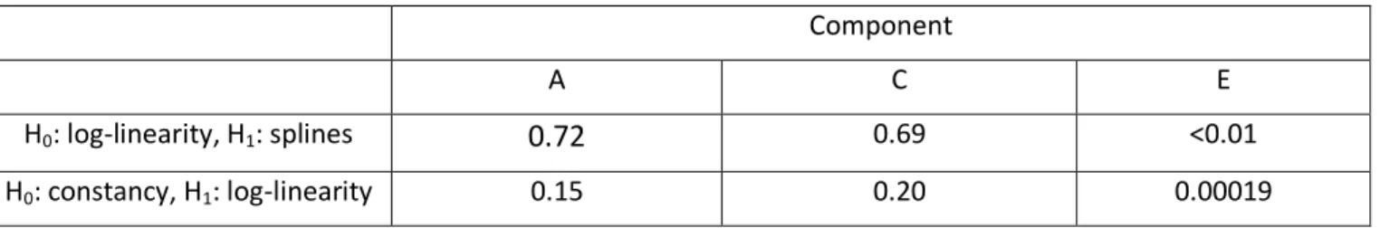
Table 2: P-values from testing log-linearity and constancy of the variance components for height. The tests were based on the twins with age>20. We first tested log-linearity against dynamic, and then tested constancy against log-linearity. Each component was tested with the other two components modeled as splines with 8 interior knots.

Component

A C E

H0: log-linearity, H1: splines 0.72 0.69 <0.01

Figures

Figure 1. The AMSEs for the three components (A, C, E) using the ACE(t) model with respect to sample size (5000 – 20000 twin pairs), number of the interior knots (5, 8, 12) and number of initial values attempted (2, 3, 4).

Figure 2. The AMSEs for the three components (A, C, E) using the ACE(t)-p model with respect to sample size (5000 – 20000 twin pairs), number of the interior knots (8, 12, 16, 20) and number of initial values attempted (2, 3, 4).

Figure 3: QQ Plots of p-values obtained by the bootstrap method under the null hypothesis for testing linearity of the C component. In this setting, the C variance component is a linear function ( ) and the A and E variance components are a constant ( ) under the null model. We investigate the influence on the type I error rate of different attempts of initial values. A) Left: One initial value was used in the estimation of each bootstrap sample. B) Right: Three randomly generated initial values were attempted in the estimation of each bootstrap sample.

Figure 4: QQ Plots of p-values obtained by the bootstrap method under the null hypothesis for testing linearity of the C component. In this setting, the A, C and E variance components are modeled by splines ( ), a linear function ( ) and a constant ( ), respectively, under the null model. We investigate the influence on the type I error rate of different numbers of interior knots (8, 10 and 12) for the spline term and different attempts of initial values. A) Top left: 8 knots and one initial value attempted. B) Top right: 10 knots and one initial value attempted. C) Bottom left: 12 knots and one initial value attempted. D) Bottom right: 12 knots and two initial values attempted.

Figure 5: QQ Plots of p-values obtained from 100 simulations under the null hypothesis for testing constancy of a variance component in the ACE(t)-p model. A) Left: the distribution of p-values without the correction of the variance of the estimated spline coefficients. B) Right: the distribution of p-values after correcting for the

underestimation of the variance of the estimated spline coefficients using a resampling method.

Figure 6: Empirical power curves for testing zero or constant variance components using the ACE(t) model. The statistical power was evaluated under different sample sizes (4000-12000 twin pairs). A) The power curves for testing a non-zero C component. B) The power curves for testing a non-zero C component with respect to different variances of the E component. C) The power curves for testing a constant E component. D) The power curves for testing a linear E component with respect to different variances of the C component. E) The power curves for testing a linear E component with respect to different intercepts.

Figure 7: Empirical power curves for testing constant or linear variance components using the ACE(t)-p model. The statistical power was evaluated under different sample sizes (4000-12000 twin pairs). A) The power curves for testing a constant E component. B) The power curves for testing a log-linear E component.

Figure 8: The variance curves of the A, C and E components for BMI and height estimated from the Finnish twin cohort. The shaded areas represent the 95% confidence bands. The variance curves are: A) across age 11-60 for BMI with 8 knots for each component, B) across age 11-60 for BMI with 12 knots for each component, C) across age 11-60 for height with 8 knots for each component, D) across age 11-60 for height with 12 knots for each component, E) between age 20-60 for height with 8 knots for each component, F) between age 20-60 for height with 12 knots for each component.

Figure 9: The dynamic heritability for BMI and height across age 11-60 estimated from the Finnish twin cohort. Both heritability curves were estimated using an ACE(t)-p model with 8 knots for each component. A) the heritability curve for BMI, B) the heritability curve for height.

Appendix

A. More description of the ACE(t)-p model

The ACE(t)-p model is featured by adding a penalizing term with a difference matrix for each component coefficients to the log-likelihood in ACE(t). From a Bayesian perspective, following the previous notations (He et al. 2016), it can be treated as assigning a multivariate normal prior on the spline coefficients of each component, i.e.,

,

where is the generalized inverse of the difference matrix and is the inverse of the penalizing coefficient . This means that the selection of is equivalent to choosing . We then develop an empirical Bayes method by first estimating from the marginal likelihood

.

By applying a Laplace approximation to the integral, we construct an EM-like algorithm to estimate . This integrated likelihood is somewhat different from the marginal likelihood used by (Ruppert et al. 2003) and (Kauermann and Wegener 2011) in the sense that we further integrate out the parameters in the fixed effects (See the derivation below). The algorithm for the estimation procedure is similar to that described in (He et al. 2016). Given , we estimate the spline coefficients by calculating the mean from the conditional joint posterior distribution

using an MCMC method. The Metropolis–Hastings (MH) method that we proposed in (He et al. 2016) using an independent normal proposal distribution suffers from slow mixing when is close to zero because of the strong linear posterior correlation between the spline coefficients. In the current implementation, if is small, we first reparameterize the spline coefficients using the spectral decomposition of (described in the following section) and run the MH algorithm based on the parameter space consisting of the eigenvectors. The posterior covariance matrix estimated from the MCMC method is used to construct the pointwise CIs.

B. Detailed description of testing a log-linear component in the ACE(t)-p model

Note that a log-linear component in ACE(t)-p can be regarded as a nested model in which we have as is satisfied only if or is linear. In fact, because , the difference matrix of the second order, is a real symmetric matrix, it can be decomposed as

, in which is an orthogonal matrix consisting of the eigenvectors and

is a diagonal matrix in which s are the eigenvalues of and the last two entries are zero. The two zero eigenvalues mean that two spline coefficients corresponding to the linear term are