de la thèse
convection et sélection de scènes homogènes
Sommaire
5.1 Introduction . . . 95
5.2 Sensibilité des simulations RTTOV-CLD au schéma de convection . . 97
5.3 Sélection des scènes homogènes pour l’assimilation all-sky . . . 104
5.3.1 Comparaison des données Eumetsat/Lannion . . . 104
5.3.2 Résumé de l’article . . . 106
5.3.3 L’article soumis à AMT . . . 109
5.4 Conclusion . . . 141
5.1 Introduction
L’un des défis majeurs de la PNT dans l’assimilation des radiances infrarouges est d’iden- tifier correctement les données claires et celles contaminées par les nuages. La plupart des méthodes de détection des nuages actuellement utilisées visent à détecter les canaux clairs dans un pixel, plutôt que d’identifier uniquement les pixels qui sont exclusivement clairs pour
[Lopez et al., 2004] et [Stengel et al., 2010a] ont étudié la non-linéarité et la sensibilité des rayonnements IR affectés par des nuages multi-couches en utilisant des schémas de diagnostic des nuages et ont ainsi pu montrer des résultats encourageants en utilisant l’assimilation va- riationnelle. Une étude de faisabilité pour l’assimilation des radiances affectées par les nuages en utilisant l’approche d’assimilation all-sky, déjà mise en œuvre pour l’assimilation des micro- ondes au CEPMMT ([Bauer and Cardinali, 2010] ; [Geer et al., 2017b] ), est également menée par [Okamoto et al., 2014], [Okamoto, 2017]. C’est pourquoi l’utilisation d’un modèle de trans- fert radiatif plus sophistiqué, prenant en compte la diffusion du rayonnement par la présence d’un profil d’hydrométéores (contenu en eau liquide, contenu en eau de glace ainsi que la fraction nuageuse) se présente comme étant un élément indispensable pour aborder la problématique de l’assimilation all-sky des radiances IASI.
Pour mener cette étude, le modèle global ARPEGE a été choisi pour permettre de couvrir une grande variété de situations météorologiques avec des cas d’observations plus ou moins nuageuses. En complément du modèle de transfert radiatif RTTOV, déjà utilisé au sein du modèle ARPEGE pour la simulation en ciel clair, le module RTTOV-CLD a été utilisé pour tenir compte de la diffusion nuageuse dans les fréquences infrarouges [Vidot et al., 2015]. En utilisant les paramètres microphysiques du contenu en eau liquide et solide dans les nuages, les nuages sont mieux représentés, notamment les structures multi-couches, et il est possible alors, d’améliorer les simulations d’observations infrarouges dans ces conditions.
Nous proposons d’aborder dans ce chapitre la sensibilité des simulations issues de ce modèle RTTOV-CLD aux variables microphysiques, en utilisant des champs venant de deux sché- mas de convection différents : le schéma de convection du modèle opérationnel (ARPEGE- opérationnel), et le schéma de convection PCMT (ARPEGE-PCMT).
Deuxièmement, différentes méthodes de sélection des scènes homogènes nuageuses et claires seront évaluées. Ces méthodes sélectives sont basées sur l’utilisation de l’information AVHRR colocalisée avec IASI. Les critères ainsi définis ont été introduits dans le cycle d’assimilation 4D- VAR d’ARPEGE. Les résultats obtenus ont été rassemblés dans l’article Farouk et al (2018) soumis au journal "Atmospheric Measurement Techniques" ; un résumé de ces résultats est
à la présence de nuages au sein de IASI FOV. De ce fait ces données peuvent être utilisées dans la méthode de détection des nuages. Les propriétés statistiques de l’AVHRR, colocalisé avec IASI, se sont déjà avérées être utiles dans des méthodes de sélection des radiances affectées par les nuages dans AROME, [Martinet et al., 2013], ainsi que pour la sélection des observations claires dans le cadre des travaux de Eresmaa 2014 [Eresmaa, 2014],
5.2 Sensibilité des simulations RTTOV-CLD au schéma de convection
Afin d’évaluer l’impact des variables microphysiques fournies par ARPEGE-PCMT sur la simulation des radiances infrarouges IASI en comparaison des variables fournies par le schéma ARPEGE-opérationnel, le tableau 5.1 nous résume les différents éléments caractéristiques des deux schémas microphysiques précédemment détaillés dans le chapitre 3 :
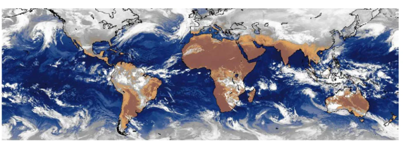
La date de 30 janvier 2017 a été choisie comme période d’étude et pour réaliser des simulations. La figure 5.1 montre les différents systèmes nuageux qui ont été observés par les imageurs en orbite géostationnaire à cette date qui a été marquée par un grand système dépressionnaire étendu du sud de l’Islande aux Iles Britanniques. On retrouve également une activité convective très forte au niveau de la Russie et de nombreux systèmes nuageux au niveau de l’océan Pacifique, du continent maritime et au nord de l’Australie. Pour rappel, au sein du modèle ARPEGE, les simulations de transfert radiatif (utilisant en entrée les variables microphysiques fournies par le schéma de convection) sont effectuées avec le modèle RTTOV-CLD pour prendre en compte la diffusion nuageuse.
Dans notre étude, seuls les pixels situés sur mer ont été traités, tout en évaluant à la fois les cas de jour et de nuit. Cependant, nous avons choisi de montrer uniquement les figures de
Potential Energy)
Convection profonde/ Diagnostiquée Simulation possible
peu profonde
Microphysique Diagnostiquée pronostique et identique
à la microphysique résolue Transport des variables Diagnostiqué Transport résolu et convectif
microphysiques par updraft et downdraft
Table 5.1 – Principales spécificités des schémas de convection de ARPEGE-Opérationnel et ARPEGE-PCMT
entre les observations et les simulations (obs - guess, appelé aussi innovation) de 314 canaux IASI le jour sur mer pour le 30 janvier 2017, en utilisant le schéma de convection ARPEGE- opérationnel (figure5.2.a), le schéma de convection ARPEGE-PCMT (figure5.2.b), ainsi que la différence entre les simulations obtenues avec chacun (figure5.2.c). Des écarts moins importants sont observés pour les canaux moins affectés par les nuages par exemple les canaux de CO2
stratosphériques (entre 657 cm−1 et 687 cm−1) et de vapeur d’eau qui pointent au-dessus de la tropopause (entre 1400 cm−1 et 1600cm−1 ).
Les écarts-types moyens obtenus avec la comparaison avec ARPEGE-opérationnel (figure5.2.a) sont plus élevés pour les canaux fenêtres sensibles à la surface, à la fois dans les conditions de ciel clair et en présence de nuages avec une valeur de 12K et un biais de -1K pour les canaux fenêtres entre 770-980 cm−1 et un écart-type de 11K avec un biais de -0,7K pour les canaux fenêtre entre 1080-1150 cm−1.
Avec ARPEGE-PCMT (figure5.2.b), on observe une hausse de 2K des écarts-types moyens pour ces canaux fenêtres cités ci-dessus. Les différences calculées entre les simulations ARPEGE- opérationnel et ARPEGE-PCMT (figure 5.2.c), montrent un biais positif indiquant de manière significative que ARPEGE-PCMT a tendance à fournir des quantités de condensats nuageux
Figure 5.1 – Composite d’images de capteurs géostationnaires pour le 30 janvier 2017 à 12 UTC
Dans la figure 5.3 nous observons que dans les régions concernées par les mers chaudes, ainsi que pour le Continent Maritime (Warm Pool), la microphysique de ARPEGE-PCMT (figure 5.3.c) permet de simuler des températures de brillances plus froides, voir trop froides avec des différences atteignant 100K, comme nous illustre la figure (5.3.c), et donc avec des phénomènes de diffusion nuageuse plus importants, par rapport à celles simulées à partir de ARPEGE-opérationnel (figure 5.3.b). L’inverse est cependant observé au nord du 20◦N, où ARPEGE-PCMT conduit à simuler des températures de brillance plus chaudes par rapport à ARPEGE-opérationnel. Les mêmes remarques ont été tirées en regardant des cas de nuit et sur mer (figures non montrées).
La figure 5.4 nous montre les différences des températures de brillance obtenues entre les observations IASI et les simulations ARPEGE-opérationnel (figure 5.4.a) et entre les observa- tions IASI et les simulations ARPEGE-PCMT (figure 5.4.b). On constate que ces différences sont très variables avec de nombreuses alternances de dipôles positifs et négatifs à très petite échelle, ce même comportement est observée pour les deux comparaison. Cependant, au niveau des tropiques on dénote une différence de comportement entre les deux comparaisons, les si- mulations de températures de brillance sont plus froides pour ARPEGE-PCMT par rapport à ARPEGE-opérationnel.
Les courbes montrant les fonctions de distribution des TB de jour et sur mer pour le canal de surface 1271 (figure5.5) font ressortir des différences notables entre les 2 sources de simulation.
(a) Schéma de convection ARPEGE-opérationnel
(b) Schéma de convection ARPEGE-PCMT
(c) différence des simulations (ARPEGE-opérationnel - ARPEGE-PCMT)
Figure 5.2 – Biais (ligne rouge continue) et écart-type (ligne pointillée verte Stdv) des dif- férences entre les observations et les simulations avec RTTOV-CLD (a) avec le schéma de convection ARPEGE-opérationnel, (b) avec le schéma de convection ARPEGE-PCMT, et (c) différence des simulations ARPEGE-opérationnel moins simulations ARPEGE-PCMT pour le 30 janvier 2017 le jour sur mer, pour 314 canaux IASI (unité : Kelvin).
(a) TB observées
(b) TB simulées avec ARPEGE-Oper
(c) TB simulées avec ARPEGE-PCMT
Figure 5.3 – Cartes de distribution de températures de brillance (TB) observées par IASI (a), simulées par ARPEGE-opérationnel (b), et simulées par ARPEGE-PCMT (c), pour le canal fenêtre numéro 1271 (962,5 cm−1) le 30 janvier 2017, de jour sur mer.
(a) ARPEGE-opérationnel
(b) ARPEGE-PCMT
Figure 5.4 – Cartes de différences des températures de brillance (TB) entre les observations IASI et ARPEGE-opérationnel (a), et ARPEGE-PCMT (b), pour le canal fenêtre numéro 1271 (962,5 cm−1) le 30 janvier 2017, de jour sur mer.
que la version opérationnelle, avec des différence de distribution pouvant atteindre 1% et de 2%
par rapport aux observations. Entre 245K et 265K nous avons une sous estimation du nombre
Figure 5.5 – Fonction de distribution des températures de brillances (TB) observées (bleu) par le canal de surface 1271 (962.50cm−1) et simulées à partir de ARPEGE-opérationnel (vert) et ARPEGE-PCMT (orange), le 30 janvier 2017, de jour et sur mer.
L’étude de l’impact du schéma de convection de PCMT sur les simulations nuageuses a permis de soulever les suppositions suivantes :
— les forts écarts-types de 12K dans ARPEGE-opérationnel et de 14K avec ARPEGE- PCMT peuvent indiquer, dans les deux cas, un problème de représentativité entre le modèle et une observation (lissage spatial) ; ceci est plus pénalisant pour ARPEGE- PCMT du fait que la convection est plus intermittente avec ce schéma.
— ARPEGE-PCMT semble sous-estimer les diffusions nuageuses dans les latitudes élevées et semble, a contrario, surestimer les phénomènes convectifs dans les Tropiques. Ces limites restent à comprendre et montrent la nécessité de mener des études plus pous- sées. De plus, le schéma de convection PCMT fut mis en suspens dans la version test
un premier temps, nous nous intéressons aux différents contrôles de qualité qui sont réalisés avant l’assimilation, et étudions la possibilité de les améliorer. Cela passe par l’utilisation du modèle de transfert radiatif (RTTOV-CLD) comme opérateur d’observation et qui va être capable de transformer les variables du modèle en radiances telles qu’elles sont observées et surtout de prendre en compte les hydrométéores (contenu en eau liquide (ql), contenu en glace (qi) et fraction nuageuse (cfrac)) pour simuler des observations nuageuses plus réalistes. En parallèle, les données des clusters AVHRR, qui sont colocalisées avec les observations IASI, vont apporter des informations précieuses sur le contenu en nuage pour chaque pixel IASI.
Avec ces nouveaux paramètres, nous avons mis en place plusieurs méthodes de sélection des observations et d’expériences d’assimilation des observations en ciel clair pour évaluer leurs impacts sur les analyses et les prévisions.
5.3.1 Comparaison des données Eumetsat/Lannion
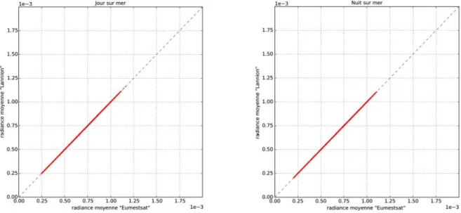
Deux centres nous fournissent les informations sur les clusters AVHRR : EUMETSAT et le Centre de Météorologie Spatiale (CMS) de Lannion. Une différence majeure entre les deux centres est que le CMS fait des acquisitions de données locales alors que les données traitées par EUMETSAT couvrent tout le globe. Une étude de comparaison de ces deux sources d’in- formation a tout d’abord été mise en place. Le premier avril 2016 est la date choisie pour effectuer cette comparaison. La première étape fut de comparer le nombre de clusters identifiés au sein des pixels IASI, puis dans un deuxième temps une comparaison de la radiance moyenne calculée pour chaque centre a été réalisée. La figure 5.6, montre au niveau de la diagonale le pourcentage d’observations présentant un nombre identique des clusters pour les deux centres EUMETSAT et Lannion, le jour et la nuit sur mer, 4% des cas présentent 1 cluster, 10% avec 2 clusters, 18% ont 3 à 5 clusetrs, et les cas de 6 clusters présentent 14% le jour et 20% la nuit.
Au-delà de la diagonale entre 19% et 20% des observations ont un nombre différent de clusters
Figure 5.6 – Comparaison du nombre de clusters AVHRR au sein des pixels IASI calculé par Eumetsat (axe X) et par Lannion (axe Y), sur mer et de jour (à gauche) et de nuit (à droite) pour le 01 avril 2016, l’échelle de couleur représente le pourcentage d’observation.
Figure 5.7 – Comparaison de la radiance moyenne pondérée des clusters du canal 11.5 µm d’AVHRR au sein de pixel IASI calculée par Eumetsat (axe X) et par Lannion (axe Y) sur
nous avons essayé dans cette comparaison d’exiger une distance maximale de 1km entre les deux produits comparés, de ce fait cette différence de nombre de clusters peut être apparue lors du mapping d’AVHRR au sein de pixel IASI des différences peuvent apparaitre.
La sélection des scènes homogènes IASI, ne peut pas se baser uniquement sur le nombre de clusters pour déterminer l’homogénéité d’un pixel IASI, et la sélection est faite en utilisant exclusivement l’information de la radiance moyenne des deux derniers canaux infrarouges de l’instrument AVHRR (10,5 µm et 11,5 µm). De cette manière, l’étude ne sera pas impactée par ce problème d’identification du nombre de clusters mentionné plus haut.
5.3.2 Résumé de l’article
En vue de préparer l’assimilation ’all-sky’ des observations IASI dans le modèle ARPEGE, et de se placer dans les meilleures conditions pour simuler les températures de brillances, une étude a été menée pour évaluer l’impact des critères d’homogénéité choisis sur les résultats d’analyse et de prévision. Cette étude est décrite en détails dans un article scientifique intitulé
’Homogeneity criteria within IASI pixels for the preparation of an all-sky assimilation’ et soumis au journal ’Atmospheric Measurement Techniques’.
Le but de cette étude est de sélectionner les scènes homogènes en utilisant les informations de colocalisation des pixels AVHRR à l’intérieur du faisceau d’observation IASI et de retenir les cas les plus favorables pour la simulation des radiances infrarouges IASI, avant de tester leurs impact dans l’assimilation actuelle d’ARPEGE.
Nous avons testé quatre méthodes de sélection de scènes homogènes en calculant des critères d’homogénéité dans l’espace d’observation ainsi que dans l’espace du modèle, à l’aide des canaux infrarouges d’AVHRR. Dans un premier temps, deux méthodes de sélection de scènes homogènes ont été proposées, en s’inspirant des critères d’homogénéités précédemment proposés dans la littérature tel que la méthode de sélection proposée par [Martinet et al., 2013] dans AROME, et celle proposée par [Eresmaa, 2014] pour la sélection du ciel clair. Ces différents
Les critères de sélection sont dérivés de Martinet et al. ( 2013) pour la sélection des scènes nuageuses dans le modèle à mésoéchelle français AROME, le canal à 11,5µm est utilisé pour réaliser trois test d’homogénéités :
1. Un test d’homogénéité intercluster, en utilisant la moyenne des radiances des clusters pour le canal de 11,5µm notée Lj pour le cluster j, ainsi que la moyenne pondérée des radiances Lmean, le critère basé surσinter est défini par :
σinter =
v u u u t
1
PCj N
X
j=1
Cj(Lj −Lmean)2 (5.1) avecCj étant la fraction nuageuse de chaque classe à l’intérieur de chaque pixel IASI, et est utilisé pour déterminer les poids. N est le nombre de classes dans un pixel IASI. Ce test est validé lorsque :
σinter
Lmean
<8%. (5.2)
2. Un test d’homogénéité intracluster est également défini dans l’espace des observations pour vérifier que chaque cluster est suffisamment homogène en utilisant la formule :
σintra =
v u u u t
1
PCj N
X
j=1
Cjσ2j (5.3)
avecσj étant l’écart-type de chaque cluster j calculé pour le canal 11.5µm). Ce test est validé lorsque :
σintra
Lmean
<4%. (5.4)
qui répondent à notre but, le premier test se situant dans l’espace d’observation et le second dans l’espace modèle, en utilisant cette fois les deux canaux AVHRR (10,5 µm et 11,5µm).
Un test d’homogénéité intercluster est appliqué en calculant l’écart-type de la température de brillance, calculé sur tous les clusters occupant le champ de vision de l’IASI. L’écart-type est calculé de la même manière que [Eresmaa, 2014] mais le pixel IASI est considéré comme homogène si les deux écart-types (un pour chaque canal) sont inférieurs à leurs valeurs seuils prédéterminées à 0,75K et 0,8K respectivement.
Le deuxième test est appliqué dans l’espace modèle, nous avons calculé le Dmean (la somme des moyennes des innovations des différents clusters) de la même manière que [Eresmaa, 2014], mais le pixel IASI est considéré comme homogène si Dmean est inférieur à 49K2.
Pour rappel Dmean est calculé de la manière suivante : Dmean =
N
X
j=1
Djfj (5.5)
où N est le nombre de clusters dans le pixel IASI, fj est la couverture nuageuse du clusterj, et Dj qui est obtenu en calculant :
Dj =X5
i=4
(Rji −RBGi )2 (5.6)
où Rji est la température de brillance du cluster j pour le canal i, et RBGi est la température de brillance simulée à partir de l’ébauche pour le canal i
Sélection des scènes homogènes en fonction de l’espace d’observation
Dans l’espace des observations (température de brillance), en utilisant les deux canaux infrarouges d’AVHRR (10,5 µm et 11,5 µm), un test d’homogénéité intercluster est proposé en évaluant la cohérence des écarts-types des clusters AVHRR au sein de pixel IASI :
L’approche de compromis pour la sélection de scène homogène
Cette méthode offre un compromis entre les différentes méthodes présentées ci-dessus. En utilisant les deux canaux infrarouges d’AVHRR (10,5 µm et 11,5 µm), deux critères d’ho- mogénéités sont définis, dans l’espace des observations et dans l’espace modèle à partir des températures de brillance. Les observations homogènes retenues pour l’assimilation doivent présenter un ratio entre le test d’homogénéité intercluster et la température moyenne inférieur à 0,8 % (Équation 5.8) ; et la somme des moyennes des innovations des différents clusters ne doit pas excéder 49 K2 (Équation5.5).
Une étude comparative entre les différentes méthodes de sélection des scènes homogènes d’IASI a fait apparaître de considérables différences dans les résultats scientifiques. Par conséquent, les critères de sélection proposés par la quatrième méthode (section 5.3.2) offrent un compromis entre les différentes méthodes, précédemment testées, en utilisant les données de température de brillance des deux canaux infrarouges d’AVHRR dans le but de définir un critère d’homogé- néité dans l’espace des observations et dans l’espace du modèle. Cette dernière méthode mène à des impacts positifs sur les différences entre les observations et les simulations statistiques, avec une proportion d’observations retenues d’environ 36% pour l’assimilation.
Ces quatre méthodes de sélection de scènes homogènes ont toutes été implémentées dans le modèle global ARPEGE en complément du système de sélection de données actuel basé sur le schéma de détection nuageuse de [McNally and Watts, 2003], et dans le but de les tester et d’améliorer le contrôle qualité de l’assimilation en ciel-clair. Les résultats d’impact, essen- tiellement avec les derniers critères de sélection (correspondant à la quatrième méthode), sur l’analyse ainsi que sur les prévisions sont plutôt de légèrement bons à neutres.
5.3.3 L’article soumis à AMT
Homogeneity criteria within IASI pixels for the preparation of an all-sky assimilation
Imane Farouk1, Nadia Fourrie1, and Vincent Guidard1
1CNRM UMR 3589, Université de Toulouse, Météo-France, CNRS, Toulouse, France Correspondence:Nadia Fourrié ([email protected])
IASI, homogeneous scenes, clouds, assimilation, ARPEGE model
Abstract.This article focuses on a selection of satellite infra-red IASI observations and their simulation in the global Numeri- cal Weather Prediction (NWP) system ARPEGE (Action de Recherche Petite Echelle Grande Echelle), using the sophisticated radiative transfer model RTTOV-CLD which takes into account the cloud multi-layers and the cloud scattering from atmo- spheric profiles and cloudy microphysical parameters (liquid water content, ice content and cloud fraction). The aim of this 5
work is to select homogeneous scenes by using information of the collocated Advanced Very High Resolution Radiometer (AVHRR) pixels inside each IASI field of view and to retain the most favourable cases for the assimilation of IASI infrared radiances. Two methods to select homogeneous scenes using homogeneity criteria already proposed en the literature were employed; criteria derived from Martinet et al. (2013) for cloudy sky selection in the French mesoscale model AROME (Ap- plications of Research to Operations at MEsoscale), and the criteria from Eresmaa (2014) for clear sky selection in the global 10
model IFS (Integrated Forecasting System). An intercomparison between these methods reveals considerable differences, ei- ther in the method to compute the criteria or in the statistical results. From this comparison a revised method is proposed that is a compromise between the different tested methods, using the two infrared AVHRR channels to define the homogeneity criteria in the brightness temperature space. This revised method has a positive impact on the observation statistics minus the simulation statistics, while retaining 36% observations for the assimilation. It was then tested in the NWP system ARPEGE 15
and tested for the clear-sky assimilation. These criteria were added to the current data selection based on the Mc Nally and Watts (2003) cloud detection. It appears that the impact on analyses and forecast is rather neutral.
1 Introduction
Satellite observations are currently the dominant source of information for Numerical Weather Prediction (NWP) systems.
Their assimilation together with in-situ observations give the atmosphere analysis, which is a necessary step in the definition 20
of the initial conditions of the forecast. This analysis consists in finding a state of the atmosphere that is compatible with the different sources of observations, the dynamics of the atmosphere and a previous state of the model. In the Météo-France global model ARPEGE (Action de Recherche Petite Echelle Grande Echelle, Courtier et al. (1991)), 70% of used observations come from infrared hyperspectral sounders, of which IASI (Infrared Atmospheric Sounding Interferometer, Cayla (2001) fills a large part. This sounder provides information about the atmospheric temperature and humidity and through its window channels 25
information about the land surface parameters in clear sky or cloudy parameters can be obtained. However, the wealth of information provided by this type of sensor with its large number of channels or radiances (8461 per pixel in the case of IASI) and its overall coverage with a horizontal resolution of 12 km at nadir, is far from being fully exploited. Indeed, the presence of clouds in the instrument field of view, which affects the majority of observations, prevents from an accurate simulation of the radiances. In fact, NWP centres use only a small amount of observations from these sounders mostly in clear sky avbove 5
clouds. Previous studies have shown that sensitive areas are often covered by clouds (McNally (2002), Fourrié and Rabier (2004)) and different techniques have been developed in the frame of global models to use infrared radiances in these regions.
In the past, different approaches have been proposed for cloud detection. A method to detect clear channels from high- resolution IR spectral instruments was proposed by McNally and Watts (2003) to assimilate channels unaffected by clouds.
At the Met Office, Pavelin et al. (2008) showed that it was possible to assimilate cloud-affected infrared radiances when 10
retrieved cloud parameters are used as set constraints. The cloud-top pressure (CTOP) and the effective cloud fraction (Ne) are firstly retrieved by a one-dimensional variational data assimilation system (1D-Var) and then provided to four-dimensional variational data assimilation (4D-Var) for the assimilation of cloud-affected infrared radiances. The analysis is significantly improved over the first guess by this method and it is used operationally to assimilate AIRS and IASI cloud-affected radiances.
At ECMWF (European Centre for Medium-Range Weather Forecasts), McNally (2009) proposed a method based on two cloud 15
parameters (CTOP and Ne) to assimilate cloud-affected IR radiances directly. In that case, the cloud parameters are determined with two channels and they are then introduced into the analysis control vector of the 4D-Var system of the global NWP model.
to constrain the minimization.
At Météo-France, the cloud parameters (CTOP and Ne) are retrieved for AIRS and IASI cloud-affected radiances with the CO2-slicing method Menzel et al. (1983). Channels affected by clouds, with the values of cloud top pressure (CTOP) ranges 20
from 650–900 hPa with a effective cloud fraction (Ne) of 1, are assimilated in addition to clear ones in the ARPEGE 4D-Var and the AROME (Applications of Research to Operations at MEsoscale) 3D-Var Pangaud et al. (2009) and Guidard et al.
(2011).
As pointed out by Errico et al. (2007), studies on the assimilation of clouds and precipitation from satellite sensors have started in the 80s and despite the encountered difficulties to implement them, operational weather centres are now assimilating 25
them with a clear benefit for the forecast quality. Efforts started with microwave radiances and direct all-sky microwave radi- ance assimilation is effective at ECMWF (Bauer et al., 2010) since 2009 and at NOAA (National Oceanic and Atmospheric Administration) NCEP (National Centers for Environmental Prediction) since 2016. Even though ECMWF focussed on the as- similation of microwave imaging and humidity-sounding channels and NOAA NCEP, on the contrary, of temperature channels from Advanced Microwave Sounding Unit-A (AMSU-A), both centres noticed benefits of such an all-sky assimilation on the 30
forecast quality (Geer et al., 2017; Zhu et al., 2016).
Concerning infrared radiance all-sky assimilation, no operational centre is yet to assimilate infra-red observations but re- search has still started in this area. Many aspects have already been studied as the information on cloud microphysics brought by the adjoint sensitivity in the assimilation (Greenwald et al., 2002) or by the retrieval of cloudy infrared radiances (Martinet et al., 2013). In addition the sensitivity, the reproducibility and the nonlinearity of the simulation of IR radiances in the presence 35
of multi-layer clouds was studied using diagnosed cloud schemes (Chevallier et al., 2004) and (Stengel et al., 2010). These studies also showed beneficial results. A step further was achieved with the study by Okamoto et al. (2014). They studied the assimilation of multi-layer cloud-affected infrared radiances using the all-sky assimilation approach already implemented for microwave imager at ECMWF. They particularly investigated the cloud effects on the differences between observations and simulations and thus proposed an appropriate quality check and dedicated observation errors.
5
In this study we are interested in IASI observations, where the radiances are considered with colocated clusters statistical properties of the Advanced Very High Resolution Radiometer (AVHRR) co-located with IASI on the METOP platform with a horizontal resolution of 1km at nadir (Cayla, 2001). Intuitively, collocated AVHRR data provide information on surface properties and the presence of clouds in the IASI Field Of View (FOV). They can therefore be used for cloud detection. The AVHRR cluster information associated with IASI has already proven to be useful for selection purposes in the context of 10
cloud data assimilation, with an explicit treatment of microphysical variables in the AROME model by Martinet et al. (2013).
Eresmaa (2014) at ECMWF also used AVHRR cluster information for cloud detection and observation selection in clear sky.
Martinet et al. (2013) selected cloudy scenes based on cloud homogeneity. This study was done in a 1D-Var framework using an advanced radiative transfer model (RTTOVCLD) including profiles for liquid water content, ice water content and cloud fraction to simulate cloud-affected radiances as background equivalents to AROME fields. The persistence of cloud information 15
brought by the analysis of cloud variables during a 3h forecast has then been evaluated successfully with an one-dimensional model AROME version (Martinet et al., 2014).
In this article, we try to determine whether or not collocated AVHRR and IASI information would facilitate the selection of homogeneous scenes which could be potentially used in an all sky assimilation approach. Section 2 describes the ARPEGE NWP system, the IASI instrument and the radiative transfer model RTTOV-CLD in cloudy sky conditions. In section 3, infor- 20
mation about the AVHRR clusters is detailled, the strengths and weaknesses of the different methods to select homogeneous observations are discussed, the chosen method is presented together with a description of the selected observations. Section 4 depicts the impacts on analyses and forecasts of selected clear and cloudy IASI observations. Conclusion and perspectives are given in section 5.
2 Experimental framework 25
2.1 The ARPEGE model and its 4D-Var system
The ARPEGE model is the global NWP model at Météo-France, used operationally since the early 1990s (Courtier et al., 1991). This system is fully integrated within the ARPEGE-IFS software that was conceived, developed and maintained in collaboration with ECMWF.
This model is a spectral global model with a stretched grid having a horizontal resolution around 7.5 km over France and 30
37 km over the antipodes. It has 105 vertical levels according a following-terrain pressure hybrid coordinate, with the first level at 10 m above the surface and an upper level at around 70 km. Clouds and precipitation are described by using three different scheme in the ARPEGE model. The stratiform clouds in terms of cloud profile and precipitation are explicitly modeled from
the microphysical condensation scheme by Lopez (2002). The large-scale effects of deep convection are parametrized from a mass-flux scheme derived from Bougeault (1985) and the shallow convection ones with the Bechtold et al. (2001) one. In these last two cases, the cloud fraction and the liquid water, ice and precipitation profiles are diagnosed.
ARPEGE has four analyses per day at 00, 06, 12 and 18 UTC. Since June 20th, 2000 the operational data assimilation system of the ARPEGE model is a 4D-Var. This implementation, as detailed in Janiskova et al. (1999) and Rabier et al. (2000), is used 5
to provide an analysis which corresponds to the best atmospheric state knowing observations, an a-priori state, dynamical and physical constraints. The background error statistics are derived from a climatological matrix and an 25-member assimilation ensemble which runs for every analysis times. The control variables considered are temperature, specific humidity, vorticity, divervence and the logarithm of the surface pressure.
At each analysis around 7 million observations are assimilated. They include conventional observations (from radiosound- 10
ing, aircraft, ground stations, ships, buoys, etc.) and satellite data. These latter include radiances in the infrared and micro- wave spectra such as AIRS (Atmospheric InfraRed Sounder), IASI, CrIS (Cross-track Infrared Sounder), SEVIRI (Spinning Enhanced Visible and InfraRed Imager), AMSU-A (Advanced Microwave Sounding Unit-A), MHS (Microwave Humidity Sounder), ATMS (Advanced Technology Microwave Sounder) and atmospheric motion vectors. Scatterometers provide infor- mation on ocean surface wind. Zenithal total delay signals and from radio-occultation measurements from the Global Naviga- 15
tion Satellite System (GNSS) are also assimilated.
With the advent of hyperspectral sounders such as AIRS and IASI, a variational bias correction (VarBC) method (Auligné et al., 2007) has been operationally implemented at Météo France and notably in the ARPEGE model. The VarBC scheme aims to minimize systematic innovations in radiances while preserving the differences between the background and other observations in the analysis system.
20
The observation operator translates the atmospheric variables quantities into the measured quantities for comparison with the actual measurements. For satellites radiances, it includes a radiative transfer model. It has then some limitations. Indeed, several atmospheric conditions are difficult to model and impose to exclude them in the assimilation process. The infrared radiances as IASI observations affected by clouds must be treated more carefully than in clear-sky conditions as their modelisation is more difficult.
25
The assimilation of clear radiances at Météo France is based on the McNally and Watts cloud detection scheme (McNally and Watts (2003)) which was designed to detect and isolate cloudy radiances from the clear-sky spectrum for a particular pixel. The method consists in finding the altitude at which the cloud affects the radiances and in filtering out the contaminated channels. The observed spectrum is compared to a clear sky simulated spectrum from the model guess. Channels are ordered according to their altitude sensitivity. This ranked partition is computed separately for each band sensitivity (CO2, water vapour, 30
ozone. . . ). In addition, a cloud characterization is made using cloud parameters (a cloud top pressure (PTOP) and an effective cloud fraction (Ne)) deduced from aCO2-slicing algorithm ( Pangaud et al. (2009)). These two parameters are used to model the radiative impact of cloud as a single layer cloud, with an emissivity set to 1 using a clear sky radiative transfer model.
2.1.1 Main features of the IASI instrument
IASI is a key element of the Metop series payload of European polar orbiting meteorological satellites (Cayla, 2001). It was designed by CNES (Centre National d’Etudes Spatiales) in cooperation with EUMETSAT. The first flight model was launched in 2006 on board the first European meteorological satellite Metop-A in polar orbit. The second instrument, mounted on the Metop-B satellite, was launched in September 2012. The third instrument will be mounted on the Metop-C satellite, which is 5
scheduled to be launched during the Autumn 2018. The horizontal resolution of the instrument is 12 km at the nadir. IASI is dedicated to operational meteorological soundings with a high level of accuracy (specifications on temperature accuracy: 1 K for 1 km and 10% for humidity (Chalon et al., 2001)). Its measurements are also useful for atmospheric chemistry to estimate and monitor different trace gases such as ozone, methane or carbon monoxide on a global scale (Hilton et al., 2012).
10
IASI is a passive IR remote-sensing instrument using an accurately calibrated Fourier transform spectrometer to cover the spectral range from3.62µm (2760cm−1) up to15.5µm (645cm−1) with 8461 channels. Its spectral resolution is 0.5cm−1 with a spectral sampling of 0.25cm−1. The IASI spectrum can be divided into three major bands:
–from 645–1210cm−1:CO2, window and ozone channels mainly sensitive to temperature, called long-wave (LW) channels;
15
–from 1210–2040cm−1: channels mainly sensitive to humidity, called water-vapour (WV) channels;
–from 2040–2700cm−1: named short-wave (SW) channels.
Only a subset of 314 channels (300 channels selected by Collard (2007) and 14 additional channels for monitoring purposes) used in operations at Météo-France, is considered in this study
2.1.2 Towards the assimilation of cloudy infrared IASI radiances 20
Assimilation of cloudy radiances is a crucial challenge for NWP centres as the cloudy observations discard represent an underexploitation of hyperspectral sounders and an error source in sensitive meteorological areas (McNally, 2002; Fourrié and Rabier, 2004). As mentioned in the introduction, studies about all-sky infrared assimilation have started. The radiative transfer model RTTOV-CLD for cloudy sky, included in RTTOV version 11 (Saunders et al., 2013), offers a realistic modeling of the cloud scattering. This model also allows to better describe the cloud emissivity as well as cloud scattering, using the 25
microphysical cloud profiles (water content, cloud ice content and cloud cover).
To simulate the radiances observed in cloudy conditions using RTTOV-CLD, we use two main types of clouds: firstly liquid water cloud, which corresponds to the Stratus Continental and Stratus Maritime ; secondly the ice water cloud of the Cirrus type, using Baran parameterisation (Vidot et al., 2015) to define the optical properties.
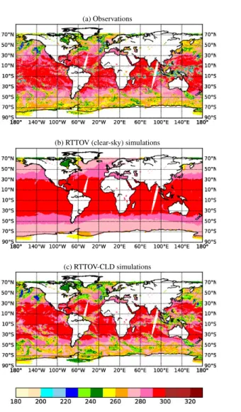
To illustrate the benefit brought by RTTOV-CLD, Figure (1) shows IASI brightness temperature observations of a cloud- 30
sensitive surface channel (1271, 962.5cm−1) and corresponding simulations with RTTOV considering clear-sky and RTTOV- CLD. Brightness temperatures less than 250 K are usually associated with higher elevation cloud structures. By using RTTOV
in clear sky (figure 1.b) to simulate IASI observations, despite the presence of some cases with almost similar values, many cloud structures are not well simulated due to the lack of cloud information in the radiative tranfer simulation. On the other hand, when IASI observations are simulated using RTTOV-CLD (figure 1.c), a good agreement is obtained and similar cloud structures are found, for example, over the North Atlantic (30N-70N, 40W-0W) and above (30S-70S, 60W-0W) the Southern Atlantic Ocean. In this case, clouds in mid-latitudes are better simulated than in the Tropics. This may be explained by the fact 5
that clouds are better simulated in the ARPEGE model for mid-latitudes than in the Tropics.
3 Selection method of homogeneous observations
The assimilation of cloudy radiances in NWP models remains an innovative challenge. In the context of the preparation of all-sky assimilation, we plan to assimilate clear or cloudy observations that are completely covered the IASI FOV in a ho- mogeneous way, discarding the cases of fractional cloud observations. These scenes are supposed to be better characterized 10
and simulated than fractional cloudy scenes in NWP models. Indeed, by selecting homogeneous cloudy scenes in both model and observation spaces, we improve the agreement between observations and background simulations. This selection of cases seen as homogeneous by both IASI and the model avoids misplacement errors. In this section, limited to cases over sea to avoid problems related to the land surface properties, we describe several methods for analysing the homogeneity of the scene in the observation and model space. However these methods were applied over all surface in the assimilation experiments of 15
section 4.
3.1 AVHRR clusters
In order to select homogeneous pixels, the AVHRR imager information collocated within IASI on the MetOp platform is used.
The spatial resolution of AVHRR observations is around 1 km at nadir and measures the radiation emitted in six broad-band channels: one visible channel, two near-infrared channels, a shortwave infrared channel and two long-wave infrared channels 20
(10.5µm and11.5µm). Two IASI Level 1c products provided by EUMETSAT were used: the AVHRR clusters (Cayla, 2001) and the percentage of cloudy AVHRR pixels in the IASI FOV (product GEUMAvhrr1BCldFrac:Pequignot and Lonjou (2009)).
The AVHRR pixels are clustered into homogeneous classes in the radiance space, (visible and infrared channels) using the K- mean classification algorithm. For each AVHRR cluster and each AVHRR channel, the mean radiance, the standard deviation and the class coverage in the IASI FOV are given.
25
3.2 Selection criteria for homogeneous observations
This study intends to focus on those IASI pixels that contain only one cluster, which corresponds to a homogeneous scene.
However only 2% of daytime IASI observations over sea contain only one class. The aggregation is built with all available AVHRR channels (visible, NIR, IR), several classes can be produced with the K-mean classification even with relatively small standard deviations for the IR channels. An IASI FOV with several classes, each one having a small standard deviation and a 30
mean radiance close to the ones of the other classes, can thus be more homogeneous than a FOV with a single class.
(a) Observations
(b) RTTOV (clear-sky) simulations
(c) RTTOV-CLD simulations
Figure 1.IASI brightness temperature (K) observations (a) from Metop A and B satellites and corresponding simulations using RTTOV (b) and RTTOV-CLD (c) for surface channel (1271, 962.5 cm−1) for 30 January 2017 daytime over sea from ARPEGE 6-hour forecast fields.
For this reason, the number of AVHRR clusters within each IASI pixel has not been used as a homogeneity criterion, but these characteristics have been used to calculate the overall AVHRR cluster statistics, aggregating the information provided by all clusters in the IASI FOV.
We tested four methods for selecting homogeneous scenes by calculating homogeneity criteria in the observation space as well as in the model space, using the AVHRR channels. The first two ones are described in the literature and we propose two other ones which are detailed below.
3.2.1 Homogeneity criteria derived from Martinet and al., (2013)
These homogeneity criteria are based on a single AVHRR infrared channel11.5µm, which is used to compute three homo- 5
geneity tests, the first two tests are calculated in the observation space and the third one in the model space:
Intercluster homogeneity
The intercluster homogeneity is based onσinterdefined as:
σinter= v u u t
1 PCj
N
X
j=1
Cj(Lj−Lmean)2 (1)
WhereLjis the mean radiances of clusterjat channel11.5µm ,Lmeanrepresents the radiance weighted average. The 10
weighting is determined byCjis the cluster fraction of each class inside the IASI pixel.Nis the number of classes in the IASI pixel.
A small calculed standard deviationσintermeans that all classes observe a similar cloudy scene in the infrared channel. If this standard deviation is too high, each class observes a different scene (clear or cloudy) and the IASI pixel is very heterogeneous.
Intracluster homogeneity 15
In order to finalize the homogeneity criterion in the observation space, it is also necessary to check if each class itself is sufficiently homogeneous, using the following formula:
σintra= v u u t
1 PCj
N
X
j=1
Cjσj2 (2)
Where theσjare the standard deviations of each clusterjcalculated for the infrared channel11.5µm. The IASI observation is considered homogeneous if it verifies the following criteria:
20
–Ratio between intracluster homogeneityσintraand mean radianceLmean< 4%.
–Ratio between intercluster homogeneityσinterand mean radianceLmean< 8%.
Background departure check
Finally, in order to obtain a similar criterion in the model space, each AROME grid point within IASI FOV was used to simulate the equivalent AVHRR channel11.5µm with RTTOV-CLD. Homogeneous IASI observations are preserved if the ratio of the standard deviation of the AVHRR simulations and the simulated mean radiance of the AVHRR is less than 8%.
Adaptation of the method 5
In our study, which focuses on the ARPEGE global model, we chose to use the simulated brightness temperature from the guess profiles coming from a 6-hour forecast and interpolated using 12 points surrounding the observation position. The homogeneous cases are retained as long as the difference between AVHRR observations and simulations is less than 7 K. This method will be noted M2013.
3.2.2 Homogeneity criteria derived from Eresmaa (2014) 10
The study of Eresmaa (2014) aimed to propose an imager assisted cloud detection for the global ECMWF NWP system and was based on the hypothesis that each AVHRR cluster are made of fully clear or fully cloudy pixels.
Therefore, his selection criteria is only intended to diagnose and retain observations when they were completely clear, using the last two infrared channels of AVHRR (10.5µm and11.5µm). This detection is based on three checks called the homogeneity check, the intercluster consistency check and the background departure check. If a IASI pixel do not satisfy one 15
of these checks, it is not free of cloud and is rejected.
The standard deviation of the brightness temperatures of the two infrared channels from all pixels present in the FOV is used for the first check. If both standard deviations are over the pre-determined threshold values (0.75 and 0.80 K, respectively), it means that a cloud is potentially observed and the IASI observation is rejected.
The intercluster consistency check relies on the comparison between the properties of the different clusters within the IASI 20
FOV. The distance of each cluster to the background in both infrared AVHRR channels as well as the distance between each pair of clusters. A cloud is detected if there is a pair of clusters covering more than 3% of the IASI FOV and for which the intercluster distance exceeds the minimum value of the distances between these clusters and the background.
The distance between 2 clustersjandkis computed as the squared-summed intercluster departure:
Djk=
5
X
i=4
(Rji−Rki)2 (3)
25
whereRji is the mean brightness temperature of clusterjfor channeli. In addition the distance of the clusterjto the background is computed with:
Dj=
5
X
i=4
(Rji−RBGi )2 (4)
WhereRBGi is the background brightness temperature for AVHRR channeli. The observation is rejected due to the diag- nostics of the presence of a cloud if the following inequality is true and the coverage of clustersjandkis over 3%:
Djk> min(Dj, Dk) (5)
The last check on the background departure is computed as a fractional-weighted mean of the squared-summed background departures:
5
Dmean=
N
X
j=1
Djfj (6)
whereN is the number of clusters in the IASI FOV andfjis the fractional coverage of clusterj. The presence of cloud is diagnosed ifDmeanexceeds the threshold value of 1K².
Adaptation of the method
Since this method assumes that each cluster is made of pixels that are either all clear or cloudy, its homogeneity tests have been 10
adapted to the selection of clear and cloudy pixels, with criteria that would fit our purpose, with the first test in the observation space and the second one in the model space. Selection thresholds were modified and all simulations from background made with RTTOV-CLD.
–Inter-cluster homogeneity. This test uses the standard deviation of the infrared brightness temperature, calculated on all clusters occupying the IASI field of view. The standard deviation is calculated in the same way as Eresmaa (2014) 15
but the IASI pixel is considered homogeneous if the two standard deviations (one for each channel) are below their predetermined threshold values of 0.75 K and 0.8 K respectively.
–Background departure check. In this test, we used theDmeanproposed by Eresmaa (2014) but the IASI pixel is consid- ered as homogeneous ifDmeanis less than 49 K².
This method is referenced as E2014 in the following.
20
The threshold values of the homogeneity criteria derived from Martinet et al. (2013) and Eresmaa (2014), are based on the analysis of statistics, applied to all IASI FOVs of the different situations (day/night at sea). Threshold values are specified in such a way that the standard deviation between the observations and simulations is not too large while keeping a fair amount of the observations.
3.2.3 Selecting homogeneous scenes in observation space 25
This third method, (called Obs_HOM thereafter) proposes a homogeneity check in the brightness temperature space calculated only on the observation space, using both infrared AVHRR channels (10.5µm and11.5µm). This inter-cluster homogeneity
criterion is based on the relative standard deviation of AVHRR clusters inside the IASI pixel. This test is satisfied when all classes observe a very similar scene in the AVHRR infrared channels. To evaluate the interclass homogeneity, the standard deviation of the mean brightness temperature of clusters which occupy the IASI FOV has been calculated using the following formula:
σinter= v u u t
1 PCj
N
X
j=1
Cj(Ri,j−Ri,mean)2 (7)
5
Where:Ri,jis the mean brightness temperature of clusterjon channeli,Ri,meanrepresents the weighted average on channeli,Nis the number of classes in the IASI pixel, andCjis the cloud fraction.
0.0 0.1 0.2 0.3 0.4 0.5 0.6 0.7 0.8 0.9 Ne IASI
0.00.5 1.01.5 2.02.5 3.03.5 4.04.5 5.05.5
Relative AVHRR standard deviation of the mean radiances (channel 10.5 µm)
0 5 10 15 20 25 30 35 40
% (a)
0.0 0.1 0.2 0.3 0.4 0.5 0.6 0.7 0.8 0.9 Ne IASI
0.00.5 1.01.5 2.02.5 3.03.5 4.04.5 5.05.5
Relative AVHRR standard deviation of the mean radiances (channel 11.5 µm)
0 5 10 15 20 25 30 35 40
%
(b)
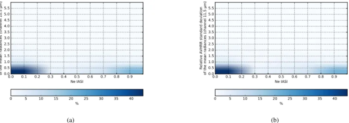
Figure 2.Density plot of the values of effective cloud fraction retrieved from IASI by aCO2-slicing algorithm (on the abscissa) with respect to the relative cluster standard deviation of the mean radiances (on the y-axis) for intercluster homogeneity for (a) the AVHRR IR Channel (10.5µm) and (b) the AVHRR IR Channel (11.5µm)
Figure 2 provides a calibration to determine the thresholds to be used to define homogeneous scenes. These thresholds should lead to a sufficient size of the selected dataset and avoid selecting the fractional cloud as much as possible. Therefore we decided to select an observation if the relationship between intercluster homogeneity and mean radiance for both AVHRR 10
IR channels (10.5µm and11.5µm) are less than 0.8%.
3.2.4 Compromise for the homogeneous scene selection
Based on the previous methods, we propose a fourth one which represents a compromise between them. Two AVHRR infrared channels (10.5µm and11.5µm) are used, and we define two homogeneity criteria in the observed and simulated brightness temperature spaces.
15
The first criterion for homogeneity is the interclass homogeneity check which was used in the third method, calculated in the observation space (presented in section 3.2.3). Similarly, in model space, we usedDmean(presented in section 3.2.2).
Methods Literature AVHRR channels Homogeneity criteria Test on background simulation used in observation space
M2013 Martinet et al. (2013) 11.5µm intra and intercluster distance with observation E2014 Eresmaa (2014) 10.8 and 11.5µm intercluster average distance with each cluster
Obs_HOM 10.8 and 11.5µm intercluster No
COMPR 10.8 and 11.5µm intercluster average distance with each cluster
Table 1.Summary of the criteria for homogeneous IASI observation selection used in this study.
Only observations that fulfilled the two following criteria were selected:
–Ratio between intercluster homogeneity and mean radiance for two AVHRR IR channels (10.5µm and11.5µm) < 0.8%.
–Sum of the average distances between each cluster and the background < 49 K².
This method is named COMPR in the following. All the four methods are sumerized in Table 1.
4 Inter-comparison of selection criteria 5
We applied our selection criteria on January 30, 2017 and result from an observation sample composed of 59,040,599 IASI FOV during the daytime over the sea are presented. Same conclusions were found for the other cases (night-time and/or over land).
To ensure that the monitoring is focused on overcast and clear scenes, the percentage of cloudy AVHRR pixels in the IASI field was used to assess the choice of homogeneity criteria.
10
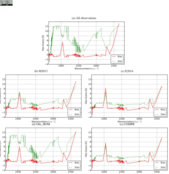
Our dataset is made of 50% of the observations entirely covered by clouds and 12% of clear observations according to the AVHRR cloud cover. The bias and standard deviation of observations minus simulations (O-G), are shown in Figure 3.(a) for the 314 IASI channels. As expected, the best statistics are obtained for channels less affected by clouds (e. g. CO2 and water vapour high peaking channels).
The mean standard deviations are larger for window channels sensitive to the surface, therefore to the presence of clouds:
15
11.7 K with a bias of -0.6 K for window channels between 770-980cm−1and 11.0K with a bias of -0.7 K for window channels between 1080-1150cm−1. Channels between 650-770cm−1show an averaged standard deviation of 2.5 K and a bias of 0.06 K.
The M2013 selection method (figure 3. (b)), reduces the standard deviation of 3.7 K with a bias of -0.16 K and to a standard deviation of 3.6 K with a bias of -0.37 K for window channels between (770-980cm−1) and (1080-1150cm−1), respectively.
20
For brightness temperature channels in the range between (650-770cm−1), we obtain a standard deviation of 0.8 K with a bias of 0.14 K. The E2014 selection method (figure 3. (c)) improves the bias to 0.11 K and -0.16 K with a standard deviation of 2.0 K for the window channels between (770-980cm−1) and (1080-1150cm−1), respectively, while the standard deviation of
(a) All observations
1000 1500 2000 2500
Wavenumbers [cm−1] 4
2 0 2 4 6 8 10 12
Obs-Guess [K]
Bias Stdv (b) M2013
1000 1500 2000 2500
Wavenumbers [cm−1] 4
2 0 2 4 6 8 10 12
Obs-Guess [K]
Bias Stdv
(c) E2014
1000 1500 2000 2500
Wavenumbers [cm−1] 4
2 0 2 4 6 8 10 12
Obs-Guess [K]
Bias Stdv (d) Obs_HOM
1000 1500 2000 2500
Wavenumbers [cm−1] 4
2 0 2 4 6 8 10 12
Obs-Guess [K]
Bias Stdv
(e) COMPR
1000 1500 2000 2500
Wavenumbers [cm−1] 4
2 0 2 4 6 8 10 12
Obs-Guess [K]
Bias Stdv
Figure 3.Bias (red solid line) and standard deviation (green dashed line) in Kelvin (K) of the differences between IASI observations and background simulations using RTTOV-CLD and a 6-hour forecast: (a) for the whole dataset, (b) after applying the homogeneity criteria derived from (Martinet et al., 2013), (c) after applying the homogeneity criteria derived from (Eresmaa, 2014), (d) after applying the selecting homogeneous scenes based on observation space, (e) after applying the compromise to select the homogeneous scenes. Observations are for January 30, 2017.