1
Supplementary Information
Effect of aging on thermal conductivity of fiber-reinforced
aerogel composites: an X-ray tomography study
Subramaniam Iswara,b, Michele Griffac,d, Rolf Kaufmannd, Mario Beltrand, Lukas Hubera, Samuel Brunnera, Marco Lattuadab, Matthias M. Koebela* and Wim J. Malfaita*
a
Laboratory for Building Energy Materials and Components, Swiss Federal Laboratories for Materials Science and Technology, Empa, Überlandstrasse 129, 8600 Dübendorf,
Switzerland
b
University of Fribourg, Department of Chemistry, Chemin du Musée 9, 1700 Fribourg, Switzerland
c
Concrete/Construction Chemistry Laboratory, Swiss Federal Laboratories for Materials Science and Technology, Empa, Überlandstrasse 129, 8600 Dübendorf, Switzerland
d
Center for X-ray Analytics, Swiss Federal Laboratories for Materials Science and Technology, Empa, Überlandstrasse 129, 8600 Dübendorf, Switzerland
*Corresponding authors: [email protected], [email protected].
Table of contents
1. Sample appearance
2. SEM images
3. Conventional Micro-CT setup
4. 3D image analysis
5. 3D volume rendering
6. Thermal conductivity of PES-silica aerogel composites 7. Thermal conductivity of silica aerogels
2
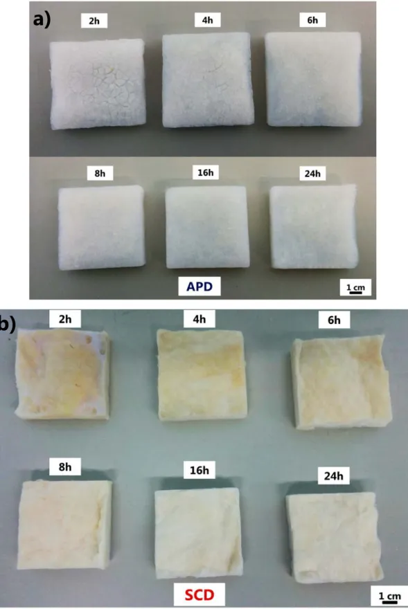
1. Sample appearance
Figure S1. (a) Ambient pressure dried (APD) PES-silica aerogel composites and (b) supercritically dried (SCD) glass wool-silica aerogel composites for different aging times.
a)
3
2. SEM images
Figure S2. SEM images of (a) 24 hours aged APD silica aerogel [1]; (b) 24 hours aged APD, (c) 2 hours aged SCD and (d) 24 hours aged SCD glass wool-silica aerogel composites.
3. Conventional Micro-CT setup
4
4. 3D image analysis
The 3D image analysis workflow applied to the X-ray tomogram of each of the 12 samples is described in Section 3.3 of the article. As described there, it was articulated in 4 main steps (Fig. 7 within the article):
(1) cropping the overall tomogram to a region-of-interest (ROI) excluding both the empty volume surrounding the sample and part of the regions containing its boundaries, because the geometrical features of the cracks in those regions may have been strongly affected by the sample preparation; it has to be noticed that with such a reduction of the tomogram sub-volume actually analysed, any pore space region is only associated to either macropores intrinsic to the aerogel matrix or cracks created by the drying shrinkage-driven cracking during the sample creation;
(2) increasing the signal-to-noise ration of the tomogram by applying to it a type of smoothing filter which selectively smoothes the 3D image only in regions and along directions characterized by very small gradients, thus allowing preserving edges corresponding to the interfaces between the three material phases in the tomographic volume (air, aerogel matrix and fibers);
(3) automatic classification of the voxels of the ROI belonging to the pore space, i.e., to the aerogel intrinsic macropores and (the majority) to the cracks;
(4) calculation of the bulk porosity, due to the aerogel macropores and to the cracks, and the cumulative size distribution of such pore space; we call such size the “crack” size 𝑆𝑆.
Step 1 was simply performed with ImageJ/Fiji [3].
Step 2 was performed with the implementation in Avizo 3D(TM) (FEI Visualization Sciences Group), version 9.2, of the Perona-Malik anisotropic diffusion filter [4]. Such implementation of that type of anisotropic diffusion filter is optimized for being run on general purpose graphics processing units (GPGPUs), providing considerable speed-up of the computation based on large scale parallelism. We run the filter algorithm on a NVIDIA Tesla K20C GPGPU card. We ran the algorithm directly using Avizo 3D’s “Filter Sandbox” module, which allows visualizing immediately the results of the filter on a small ROI of the 3D image in order to explore the effect of varying different parameter values.
5
The nonlinear diffusion partial differential equation at the basis of the Perona-Malik algorithm was solved numerically with the associated finite difference time domain scheme using 10 temporal iterations and a diffusion stop threshold value which was set independently for each tomogram based upon a visual assessment of the degree of smoothing and of edge
preservation.
Step 3 actually consisted in two sub-steps. The first sub-steps consisted of the identification of the voxels corresponding to the glass wool fibers. Such identification (segmentation) was performed by a repeated, manual selection of a range of voxel values leading to a sufficient identification of voxels belonging to the fiber material phase. Such a manual selection, typically called manual thresholding because a lower and an upper bound for the range as thresholds in voxels values are chosen directly by the image analyst. In the case of our tomograms, the selection of such threshold was rather reliable given the large mismatch in voxel values between the fibers and the other two phases, being the fibers much more X-ray attenuative than the other two phases. The manual thresholding was performed with the “Segment Phases 3D” plugin of the Empa Bundle of ImageJ Plugins for Image Analysis (EBIPIA) [5], by using the histogram of voxel values of the ROI obtained from Step 1.
A 3D binary image, also called 3D binary mask, for the fiber phase was created by the “Image Calculator” plugin of the EBIPIA, by creating a 8-bit unsigned integer image where the segmented voxels were reassigned value equal to 255 (“white” in such an image) while all the other voxels were assigned value 0. With the same plugin, we created a 3D binary mask for the aerogel + pore space, corresponding to the result of the application of a Boolean NOT operator to the previous binary mask.
The binary mask for the aerogel + pore space was used as input for the “Cluster image” plugin of the EBIPIA for the segmentation of the voxels corresponding pore space voxels, i.e., mainly to crack volume. Such mask indicated to the “Cluster image” plugin to consider only such voxels in the application of the data clustering algorithm for the segmentation.
The “Cluster image” plugin allows choosing within a broad spectrum of data clustering algorithms, where the data are pixel/voxels value from one or more 2D/3D images. Each
6
voxel, as geometric entity, is assigned one or more feature values corresponding to the voxel values in the used images. In our case, only the filtered tomogram’s voxel value was used as a definition of feature voxel variable, i.e., the feature space was a 1D Euclidean space. Data clustering falls under the category of unsupervised machine learning algorithms [6].We specifically chose the K-means clustering algorithm of Kanungo et al. [7] as implemented in the EBIPIA’s “Cluster image” plugin, looking for K=2 clusters of points in the feature space of the filtered tomogram, one cluster corresponding to the aerogel matrix phase, the other to the pore space one. The Kanungo et al. algorithm implements a classical version of the K-means data clustering approach, the Lloyd’s algorithm [8], but in a computationally efficient way, allowing achieving quickly convergence to the solution of the optimization problem at the basis of the algorithm itself.
The final output of the “Cluster image” plugin was a 3D binary mask for the pore space only which was used as the input for Step 4 of the analysis, performed with the “Pore size
distribution” EBIPIA plugin, which allowscomputing the pore (in our case crack) size distribution according to the algorithm proposed and developed by Münch and Holzer [9]. Such an algorithm relies upon a probabilistic definition of pore size, described by Torquato [10] and is particularly optimal for pore spaces consisting of pores with arbitrary shape and degree of interconnectivity.
Traditionally, a pore size distribution is calculated from the 3D binary image of a pore space by labelling it and computing for each distinct, separated and labelled pore its equivalent diameter, equal to the diameter of a sphere with identical volume as the pore, plotting at the end the histogram of the equivalent diameters of all the labelled pores. This approach is referred to as “discrete pore size distribution” by Münch and Holzer [9].Using such an approach to compute a pore size distribution leads to physically and geometrically incorrect estimates if the majority of the pore space is built up by regions which do not have shape close to a sphere.
The probabilistic approach described in [10] considers the pore space as a statistical ensemble of values for the pore(crack) size as a random variable 𝑆𝑆, where one value is associated to each pore space voxel and it is calculated as the double of the Euclidean distance transform value at that voxel. The latter variable corresponds to the maximum radius of a sphere
7
centered in that voxel and completely fitting within the pore space. Each distinct and
disconnected part of the pore space, i.e., each individual and separated pore, is characterized not by a single size but by a set of them.
Opposite to a “discrete pore size distribution”, Münch and Holzer built upon such a
probabilistic definition of size of a pore space and proposed an efficient algorithm to compute its complementary cumulative distribution function (cCDF) 𝐹𝐹�(𝑆𝑆) = 1 − 𝐹𝐹(𝑆𝑆), where 𝐹𝐹(𝑆𝑆) is the cumulative distribution function of 𝑆𝑆. Such algorithm exploits the Euclidean distance transform of the 3D binary image of the segmented pore space to compute incrementally the cumulative pore space volume fraction that can be covered by overlapping spheres with varying diameter larger than 𝑆𝑆, corresponding to the estimate of 𝐹𝐹�(𝑆𝑆).
The “Pore size disribution” plugin allows expressing 𝐹𝐹�(𝑆𝑆) also as a cumulative pore space volume fraction, i.e., porosity, 𝑐𝑐𝑐𝑐(𝑆𝑆), due to pores with size larger then 𝑆𝑆. 𝑐𝑐𝑐𝑐(𝑆𝑆) ≡ 𝐹𝐹�(𝑆𝑆) ⋅ 𝑉𝑉𝑝𝑝𝑝𝑝𝑝𝑝𝑝𝑝 𝑠𝑠𝑝𝑝𝑠𝑠𝑠𝑠𝑝𝑝/𝑉𝑉𝑅𝑅𝑅𝑅𝑅𝑅, where 𝑉𝑉𝑝𝑝𝑝𝑝𝑝𝑝𝑝𝑝 𝑠𝑠𝑝𝑝𝑠𝑠𝑠𝑠𝑝𝑝 is the total volume of the pore space, independently of the
𝑆𝑆 value (note that 𝐹𝐹�(𝑆𝑆 = 0 𝜇𝜇𝜇𝜇) = 1 based upon Kolmogorov’s basic axioms of probability theory) and 𝑉𝑉𝑅𝑅𝑅𝑅𝑅𝑅 is the total volume of the ROI produced at Step of the workflow, i.e., the total volume analyzed. 𝑐𝑐𝑐𝑐(𝑆𝑆 = 0 𝜇𝜇𝜇𝜇) is thus the porosity 𝑐𝑐 ≡𝑉𝑉𝑝𝑝𝑝𝑝𝑝𝑝𝑝𝑝 𝑠𝑠𝑝𝑝𝑠𝑠𝑠𝑠𝑝𝑝
8
5. 3D volume rendering
The file 3DRenderingFilteredVolumeWScaleBar.avi contains the animation (movie) of a computer graphics rendering of the filtered (edge-preserved smoothed) tomogram for the 2 hours aged ambient pressure dried glass wool-silica aerogel composite sample. The parts of the volume corresponding to air and aerogel matrix are assigned distinct degrees of transparency, to make the aerogel matrix and the fibers more visible. The animation consists in moving the camera in the 3D scene around the sample. The movie file is in AVI format with a frame rate of 15 fps. The first frame of the movie is shown here above.
9
The file 3DRenderingFiltVolFibersWScaleBar.avi contains the animation (movie) of the same type of computer graphics rendering of the filtered (edge-preserved smoothed) tomogram for the 2 hours aged ambient pressure dried glass wool-silica aerogel composite sample with a difference: the 3D binary image of the segmented fibers is rendered as well as overlapped on top of the tomogram and coloured in orange with a certain degree of transparency as well. While the camera rotates around the sample, the tomogram volume is gradually removed from the 3D scene by a clipping plane moving from the top to the bottom and only the rendered 3D binary mask of the fibers is left. The figure above shows a frame of such movie where almost all of the volume of the tomogram is removed and the spatial distribution of the segmented fibers within the sample is clearly visible.
10
The file 3DRenderingFiltVolFibersPoreSpaceWScaleBar.avi contains the animation (movie) of the same type of computer graphics rendering as in 3DRenderingFiltVolFibersWScaleBar.avi with the addition of the rendering of the 3D binary mask of the segmented pore (crack) space, shown in blue, also in this case with a certain degree of transparency. As the camera rotates around the sample, the rendered volume of the tomogram is also in this case removed by a sliding clipping plane, leaving in the 3D scene only the two 3D binary mask, for the fibers and the pore space, respectively.
11
6. Thermal conductivity of PES-silica aerogel composites
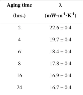
Table S1. Influence of aging time on the thermal conductivity (λ) of PES-silica aerogel composites. Aging time (hrs.) λ (mW·m-1·K-1) 2 22.6 ± 0.4 4 19.7 ± 0.4 6 18.4 ± 0.4 8 17.8 ± 0.4 16 16.9 ± 0.4 24 16.7 ± 0.4
12
7. Thermal conductivity of silica aerogels
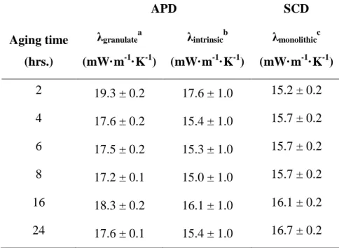
Table S2. Thermal conductivity of APD and SCD silica aerogels.
Aging time (hrs.) APD SCD λgranulatea (mW·m-1·K-1) λintrinsicb (mW·m-1·K-1) λmonolithicc (mW·m-1·K-1) 2 19.3 ± 0.2 17.6 ± 1.0 15.2 ± 0.2 4 17.6 ± 0.2 15.4 ± 1.0 15.7 ± 0.2 6 17.5 ± 0.2 15.3 ± 1.0 15.7 ± 0.2 8 17.2 ± 0.1 15.0 ± 1.0 15.7 ± 0.2 16 18.3 ± 0.2 16.1 ± 1.0 16.1 ± 0.2 24 17.6 ± 0.1 15.4 ± 1.0 16.7 ± 0.2 a
thermal conductivity of APD silica aerogel (granulate-powder mix) [11] was measured using a guarded hot plate [12].
b
intrinsic thermal conductivity of APD silica aerogel granulate was determined from the calibration curve as described by Huber et al. [11].
c
thermal conductivity of SCD monolithic silica aerogel was measured using a guarded hot plate [12].
13
8. References
[1] S. Iswar, W.J. Malfait, S. Balog, F. Winnefeld, M. Lattuada, M.M. Koebel, Microporous Mesoporous Mater. 241 (2017) 293–302.
[2] M.A. Beltran, D.M. Paganin, K. Uesugi, M.J. Kitchen, Opt. Express 18 (2010) 6423– 6436.
[3] J. Schindelin, I. Arganda-Carreras, E. Frise, V. Kaynig, M. Longair, T. Pietzsch, S. Preibisch, C. Rueden, S. Saalfeld, B. Schmid, J.-Y. Tinevez, D.J. White, V.
Hartenstein, K. Eliceiri, P. Tomancak, A. Cardona, Nat. Methods 9 (2012) 676–682. [4] P. Perona, J. Malik, IEEE Trans. Pattern Anal. Mach. Intell. 12 (1990) 629–639. [5] B. Münch, “The Empa Bundle ImageJ Plugins Image Anal. (EBIPIA),
http//imagej.net/Xlib” (2015).
[6] A.K. Jain, M.N. Murty, P.J. Flynn, ACM Comput. Surv. 31 (1999) 264–323.
[7] T. Kanungo, D.M. Mount, N.S. Netanyahu, C.D. Piatko, R. Silverman, A.Y. Wu, IEEE Trans. Pattern Anal. Mach. Intell. 24 (2002) 881–892.
[8] S.P. Lloyd, IEEE Trans. Inf. Theory 28 (1982) 129–137.
[9] B. Münch, L. Holzer, J. Am. Ceram. Soc. 91 (2008) 4059–4067.
[10] S. Torquato, in:, Random Heterog. Mater. Microstruct. Macrosc. Prop., Springer New York, New York, NY, 2002, pp. 48–50.
[11] L. Huber, S. Zhao, W.J. Malfait, S. Vares, M.M. Koebel, Angew. Chemie - Int. Ed. 56 (2017) 4753–4756.
[12] T. Stahl, S. Brunner, M. Zimmermann, K. Ghazi Wakili, Energy Build. 44 (2012) 114– 117.
![Figure S2. SEM images of (a) 24 hours aged APD silica aerogel [1]; (b) 24 hours aged APD, (c) 2 hours aged SCD and (d) 24 hours aged SCD glass wool-silica aerogel composites](https://thumb-eu.123doks.com/thumbv2/123doknet/14820461.615347/3.892.183.710.164.616/figure-images-hours-silica-aerogel-silica-aerogel-composites.webp)