Global portfolio diversification with cryptocurrencies

(1)

Faculté des sciences économiques Avenue du 1er-Mars 26

CH-2000 Neuchâtel

www.unine.ch/seco

Master thesis submitted to the Faculty of Economics and Business

Institute of Financial Analysis University of Neuchâtel

For the Master of Science in Finance by

Salma OUALI

Supervised by:

Prof. Frédéric SONNEY, University of Neuchâtel

Neuchâtel, August 2019

GLOBAL PORTFOLIO DIVERSIFICATION WITH

CRYPTOCURRENCIES

(2)

1 Abstract

This study raises questions about the potential of cryptocurrencies as a new alternative investment. I explore the ability to which major cryptocurrencies endow diversification and hedging benefits to a global investor. Using the dynamic conditional correlation model developed by Engle (2002), I find evidence of effective diversification and weak hedging effects against global traditional assets. Furthermore, I investigate the issue using risk based portfolio optimization frameworks. I find enhanced performance of the investor’s portfolio when including Bitcoin to a well-diversified portfolio. Likewise, later generation of cryptocurrencies Ripple, Dash and Litecoin provide better improvement on a risk adjusted basis. Nonetheless, their very high volatility worsen off the portfolio’s downside risk.1

1_{ACKNOWLEDGEMENTS: I would like to express my gratitude to my supervisor Prof.} Frédéric Sonney for his guidance and valuable advice. I would like to thank my family for their love and unconditional support. I am also grateful to my partner and my best friend for brightening my life throughout the thesis process.

(3)

2 1. Introduction

The 2008 financial crisis led to growing skepticism around traditional financial systems.

As a response to these backdrops, a programmer under the pseudonym of Nakamoto introduced Bitcoin, a decentralized medium of exchange in 2009. The peer-to-peer electronic currency shows unique features. It is not backed by any central authority, has a fixed supply set in advance of 21 million Bitcoins and is created via an innovative technology, Blockchain that registers transactions and stows them into transparent blocks. These blocks are completed once these transactions are verified and secured into a distributed network. Therefore, this creation process is similar to gold mining, which led to Bitcoin being called the “digital gold”.

Following the inception of Bitcoin, many alternative cryptocurrencies, using the same blockchain technology emerged. Whether addressing same purposes as Bitcoin or providing innovative decentralized solutions, they attracted investors’ attention and gained growing market shares with the most popular among them being Ethereum, Ripple, Dash, Stellar and Litecoin.

Driven by high capital inflows, Cryptocurrencies witnessed price rise in tandem. Market capitalization and volume traded continued growing exponentially until the end of 2017, when Bitcoin realized its meteoric rise before topping out in the following months.

This rapid surge in prices and the high volatility displayed by the cryptocurrency market has attracted mostly speculators seeing Cryptocurrencies as a speculative asset rather than a currency store of value. Consequently, many investors question whether cryptocurrencies are just fictitious currencies forming speculation bubbles or a valuable opportunity investment.

The main purpose of this study is to explore Cryptocurrencies as a new alternative investment.

The research is conducted from the perspective of a global investor who considers diversification as of paramount importance. Considering the excessive volatility encompassing

(4)

3

cryptocurrencies, I restrain cryptocurrencies to hedging and diversification uses only. According to Baur and Lucey (2010), a hedge is an asset that shows adverse correlation to another asset, whereas a diversifier exhibits marginal positive price co-movements with the other asset. Furthermore, this study sheds light on the use of the cryptocurrencies as performance enhancers in a global portfolio while previous research focused only on Bitcoin. I benchmark the cryptocurrency market with Bitcoin and three major alternative cryptocurrencies: Ripple, Dash and Litecoin. Whilst among traditional assets I consider stocks, bonds, real estate and gold.

In order to investigate the diversification and hedging traits of the aforementioned cryptocurrencies and capture the co-movement between each cryptocurrency and the traditional assets, I consider the multivariate dynamic conditional correlation GARCH model of Engle (2002). The results offer compelling evidence of cryptocurrencies as effective diversifiers, yet they exhibit weak hedging properties. I find that Bitcoin acts as a strong hedge only against price movements of Chinese equities, global real estate and corporate bonds. Additionally, Litecoin qualifies as a hedge for global real estate and Japanese equities. Whereas Dash is only a good hedge against global bonds. Ripple, on the other side, does not possess any hedging properties since it exhibits moderately positive correlation with all traditional assets.

I further examine the diversification perquisites of cryptocurrencies in a portfolio comprising all traditional asset classes. Bruder and Roncalli (2012) argue that risk aversion of institutional and individual investors increased significantly after the 2008 financial crisis. Thus, they prompt the use of investment strategies based on risk budgeting and diversification instead of return forecasting ones.

Regarding this matter and the high volatility nature of Cryptocurrencies, this study adopts four optimization frameworks that focus on measuring risk: traditional minimum variance, minimum conditional value at risk, inverse volatility and maximum diversification.

(5)

4

The out-of-sample performance of the optimal portfolios is studied on a risk adjusted return basis. The back-testing results confirm the evidence of cryptocurrencies being outstanding diversifiers. Regardless of the strategy, I find that adding cryptocurrencies to the basic portfolio, the risk return ratio increases significantly albeit at different magnitudes. On the other side, the downside risk of the portfolio increases especially when alternative tokens are included. Interestingly, Bitcoin succeeds to reduce the downside risk under minimum variance and inverse volatility.

The research paper is structured as follow: Section 2 presents the literature review, section 3 undergoes the methodology details, section 4 introduces the data, section 5 reports empirical results and robustness check and section 6 provides conclusion.

2. Literature review

Despite the global financial instability, the strong past financial performance of bitcoin (BTC) made it comparable to a digital gold. Therefore, a strand of studies examined Bitcoin and its properties as an asset class. Yermack et al. (2013) compare BTC’s daily exchange rates with gold and fiat currencies and argue that BTC is more comparable to a speculative investment. Baur et al. (2015) investigate statistical properties and future usage of bitcoin. They suggest that bitcoin is a hybrid between conventional currencies and commodity currency. Dyhrberg et al. (2015) find similarities of BTC with gold and USD and confirm the views of Baur et al. (2015). Ciaian, Rajcaniova and Kancs (2016) go a step further and analyze the impact of BTC’s supply and demand on its price formation. Thus, they discover similar price formation patterns with other currencies.

Whether considered as a medium of exchange or a highly speculative asset, BTC’s skyrocketing returns are the main reason of its attractiveness. After being accepted as a method of payment, its use as a financial investment vehicle has been thoroughly examined. In point of fact, a broad

(6)

5

range of literature studied whether including bitcoin in a traditional portfolio can enhance its return and reduce the risk.

Brière et al. (2015), using mean variance spanning test, assert BTC’s diversification benefits in an investment portfolio. They conclude that BTC’s low correlation with other assets enhances the portfolio’s performance and compensates for the increase in the overall risk. As returns of BTC exhibit high kurtosis and low skewness, Eisl et al. (2015), proposes the use of a CVaR framework as an alternative to mean variance analysis. Their findings are in line with the ones of Brière et al. (2015). Indeed, investing a small fraction in BTC enhances intensely the portfolio’s risk return tradeoff.

Kihoon Hang (2016), performs a trading strategy based on momentum (TSMOM). By conducting a mean variance analysis, he demonstrates that enhanced returns and reduced volatility can be achieved in a portfolio of equities and TSMOM.

Diversification and hedging are characteristics of huge importance when building a portfolio. Therefore, an investigation of correlation between BTC and other financial assets is crucial. Following this, Bouri et al. (2017), employed a dynamic conditional correlation model (Engle, 2002) to estimate correlation between BTC and other financial assets. They find that Bitcoin does qualify as an effective diversifier. However, it can only serve as a hedge or safe haven in few cases. On the contrary, Bouoiyour and Selmi (2017), vindicate the hedge and safe haven role of bitcoin against oil price movements. Moreover, by adding Bitcoin to a portfolio of oil only, they observe an enhancement in performance and downside risk reduction.

Guesmi et al. (2018), consider DCC GJR GARCH as the suitable model for modeling joint dynamics of different financial assets. They document that Bitcoin can be a systematic hedge and that adding a small fraction of bitcoin reduces considerably the portfolio’s risk exposure.

(7)

6

They also stress that a short position in Bitcoin hedges the risk for commodities, stocks and currencies.

Due to the high trading and predominant mining activity in China, Kajtazi and Moro (2017), raise the question of whether BTC adds value in a Chinese asset-based portfolio. They show significant but low correlation with Chinese assets and argue that Bitcoin fails in enhancing portfolio’s performance over all periods.

Evidence that Bitcoin offers diversification benefits in a traditional portfolio is abundant in literature and so far, research towards altcoins remains infrequent.

Aiming to close this gap, Osterrieder et al. (2016), were amongst the first to explore the interdependences between cryptocurrencies (CCs). They demonstrate that low mildly correlation exist between most CCs except for the ones sharing the same technology. Following this, Braineis and Mestel (2018), expand the research by exploring the effects of diversified cryptocurrency investments. Their empirical results show that adding several CCs expands the efficient frontier of a bitcoin-based portfolio.

Further investigating the diversification effect, Chuen et al. (2017), advocate the use of the CRIX index, which was developed by Trimborn and Hardle (2016) to mimic the CCs market performance. When looking at static and dynamic correlations between CRIX and traditional assets, they give evidence of diversification benefits. However, the mean-variance spanning tests reveal enhancement of global minimum variance only. In fact, the negative skewness of CRIX and high risk makes it redundant in a tangency portfolio.

Klein et al. (2018), argue that Bitcoin is not the new gold. According to their research results, Bitcoin is only suitable for diversification benefits and does not display stable hedging

(8)

7

capabilities. Meanwhile, they find CRIX to display better hedging effects. Yet, it still fails to be an effective hedge like gold.

3. Data

To conduct the analysis, I retrieve data from two different sources. I retrieve daily closing prices for traditional assets in form of indices from DataStream. While the data for cryptocurrencies are extracted from coinmarketcap.

According to Abidin et Al. (2004), international diversification is proven to yield higher returns and reduce risks and since cryptocurrencies are global in nature, I decide to adopt the perspective of a global investor. Therefore, I create a well-diversified international portfolio composed of cryptocurrencies and traditional assets.

Emphasis lies on the largest cryptocurrency assets. Therefore, I select four cryptocurrencies from the ten largest cryptocurrencies by market capitalization. Bitcoin and three major alternative cryptocurrencies: Litecoin, Ripple and Dash. These cryptocurrencies are portrayed as more suitable than other major altcoins like Bitcoin cash and Ethereum, which were only introduced in 2015 and 2017, respectively, and would not provide enough set of data to conduct the research. Additionally, the selection is made based on the underlying correlation of the alternative cryptocurrencies with Bitcoin. Ripple and Dash are moderately correlated with Bitcoin while Litecoin is relatively highly correlated with the latter.

Traditional and alternative assets comprise equity, fixed income, real estate and gold. Each asset class is embodied by liquid financial indices.

Equity indices are selected based on the four most important markets of cryptocurrencies trading. I use four regional indices S&P 500, Euro Stoxx 50, Nikkei 225, SSE (Shanghai Stock Exchange) as well as MSCI Emerging Markets Index. Considering the global bond universe of fixed income, I adopt the following indices: S&P Global Developed Sovereign Bond Index and

(9)

8

IBOXX Liquid Investment Corporate Grade Index. Gold is added in consonance with Dyhrberg et al. (2015) since the latter is typically depicted as hedge. As of real estate, I use as a reference FTSE EPRA NAREIT global.

The sample contains daily price information from 30 July 2014 to 31 April 2019. I remove the daily data of cryptocurrencies during the weekends in order to match the number of observations with traditional assets.

Furthermore, I compute daily log returns since they are deemed more convenient for time series analysis and provide a better fit for statistical models. Therefore, daily log returns are obtained using the following formula:

𝑟𝑖𝑡 = 𝑙𝑜𝑔 𝑝_𝑖,𝑡 𝑝𝑖,𝑡−1

4. Methodology

Modern portfolio theory states that correlation is the basis of diversification in a portfolio. Accordingly, investing in low correlated or negatively correlated assets can achieve efficient diversification (Bodie et Al, 2014). Following this, I examine diversification capabilities of cryptocurrencies as well as their ability to enhance the risk-return reward of a global investor.

4.1. Correlation analysis

I perform a correlation analysis in order to assess if cryptocurrencies can be a diversifier or a hedge. At first, I estimate correlation coefficients of cryptocurrencies and other assets via a pairwise correlation. However, the latter is only the average estimation and correlation in general is known to display time varying properties.

Hence, I conduct the multivariate dynamic conditional correlation (DCC) model by Engle (2002). The advantage of the model lies in its limited number of estimated parameters, univariate GARCH flexibility and its direct parameterization of conditional correlation.

(10)

9

The estimation of the DCC model is performed in three steps:

I estimate an ARMA (1, 1)2 mean equation to model the conditional mean and deal with the autocorrelation in the time series returns.

The conditional mean equation for each asset is presented in the equation below:

𝑅𝑡 = 𝑐 + ℰ𝑡+∑ 𝜑𝑖𝑅𝑡−𝑖+ ∑ 𝜃𝑖 𝑞 𝑖=1 𝑝 𝑖=1 ℰ𝑡−𝑖

Where c is a constant term, ℰ𝑡 is the white noise, p is the autoregressive term, q the moving average term and φ, θ are the model parameters.

After deeming the conditional mean for each asset, the ARMA residuals are used to estimate the GARCH (1, 1) variance model.

Therefore, conditional variances are implemented one by one using the following formula: 𝜎_𝑡2_{= 𝜔 + 𝛼 ℰ}

𝑡2+ 𝛽𝜎𝑡−12

Where 𝜎_t is the conditional variance, 𝜔 is the intercept, 𝛼 is the coefficient displaying the impact of previous shocks, ℰ_𝑡2 is the squared residual and 𝛽 is a coefficient that transmits the GARCH (1, 1) effect.

Afterward, I model conditional covariance of standardized returns using computed variances from first step.

With 𝜌_{𝑖,𝑗,𝑡+1} = 𝐶𝑜𝑣_𝑡(𝑧_𝑡+1𝑖 , 𝑧_𝑡+1𝑗 )₀ and 𝜌̅_𝑖,𝑗 = 𝜔 1−𝛼−𝛽

The dynamic conditional correlation is computed as follows:

𝑞_{𝑖,𝑗,𝑡+1} = 𝜌̅_𝑖,𝑗+ 𝛼 (𝑧_𝑡+1𝑖 𝑧_𝑡+1𝑗 − 𝜌̅_𝑖𝑗) + 𝛽 (𝑞_{𝑖,𝑗,𝑡}− 𝜌̅_𝑖𝑗)

(11)

10

Once the auxiliary variable 𝑞_{𝑖,𝑗,𝑡+1} is forecasted, I compute the dynamic conditional correlation as follows:

𝜌_{𝑖,𝑗,𝑡+1} = 𝑞𝑖,𝑗,𝑡+1 √𝑞𝑖,𝑖,𝑡+1√𝑞𝑗,𝑗,𝑡+1

After studying the co-movement between the selected asset classes and cryptocurrencies, I investigate the usefulness of cryptocurrencies as a diversification tool from a portfolio perspective.

4.2. Portfolio optimization

I start by constructing a portfolio without cryptocurrencies, which will be referred to as the basis portfolio. Furthermore, I investigate the options of including cryptocurrencies to the traditional assets’ portfolio. I construct two sets of portfolios. The first portfolio includes traditional assets and only Bitcoin and the second one includes traditional assets and the four cryptocurrencies. The benefits of adding cryptocurrencies are assessed in terms of risk-return profiles, cumulative wealth and downside risk.

In order to calculate these performance metrics, I use the out-of-sample backtesting method, which evaluates trading strategies using historical data. The models’ parameters are assessed via a rolling window approach under the following steps: I use the 200 last days observations before the rebalancing date for the parameters’ estimation. Then, the resulting weights are rebalanced on a monthly basis for the whole out of sample period.

Thus, the optimized weights are subject to different parameters depending on the optimization frameworks presented below.

(12)

11

4.2.1. Minimum risk approaches

Minimum variance portfolio is the Markowitz least variance framework. It is set out as the portfolio that maximizes the use of diversification to achieve the lowest risk. The portfolio weights are optimized for each point in time using the subsequent formula:

𝑚𝑖𝑛 𝜎_𝑃2 _{= ∑} _∑ _𝑤 𝑖𝑤𝑗𝜎𝑖𝑗 𝑛 𝑗=1 𝑛 𝑖=1 s. t. 𝑤𝑖 ≥ 0, ∑𝑛𝑖=1𝑤𝑖 = 1

Where weights are estimated by using the historical variance and covariance matrix.

Nevertheless, a strong shortcoming of the mean variance analysis is the assumption of normal distribution of returns. In this context, cryptocurrencies’ excess volatility infers a heavy tail distribution as already stated by Eisl et al. (2015) and Chuen et al. (2017).

To cope with this issue, I follow Rockafeller and Uryasev (2002) to construct the conditional value at risk strategy (CVaR). The strategy uses the expected shortfall, which is a more coherent risk measure contrasting to the variance since it aims to quantify only the downside risk. Log returns are simulated via a T-student distribution.

Therefore, conditional value at risk portfolio weights are given by solving the following optimization problem: min 𝑤𝑡∈𝑅𝑝 𝐶𝑉𝐴𝑅_𝛼(𝑤_𝑡) 𝑠. 𝑡. 𝑢_𝑝,𝑡(𝑤_𝑡) = 𝑟_{𝑡𝑎𝑟𝑔𝑒𝑡} ; 𝑤_𝑡1_𝑝 = 1 , 𝑤_𝑖,𝑡 ≫ 0 𝐶𝑉𝐴𝑅_𝛼(𝑤) = 1 (1 − 𝛼) ∫ 𝑓(𝑤, 𝑟)𝑝(𝑟)𝑑𝑟 0 𝑓(𝑤,𝑟)≤𝑉𝐴𝑅𝛼(𝑤)

Where f (w, r) is the probability density function of portfolio returns with weights w, 𝛼 is the confidence level, 𝑉𝐴𝑅_𝛼 is the loss to be expected in 𝛼.100% of the times.

Short selling is constrained under the two strategies since Bitcoin futures were only introduced recently on Chicago Board Options Exchange (CBOE) and Chicago Mercantile Exchange

(13)

12

(CME) in December 2017. In addition, I impose a maximum weight constraint of 50% for each asset in order to omit extreme weight allocations.

0% < 𝑊_𝑖 < 50% 4.2.2. Risk budgeting approaches

Requiring only the estimation of volatility, risk budgeting approaches are becoming a popular solution for risk adverse investors. Booth and Fama (1992) argue that these models put diversification at the heart of the investment strategy and are a good alternative to Markowitz least variance framework when the assumption of normal returns is not solid. Therefore, I adopt the subsequent risk budgeting approaches:

The inverse of the volatility is used to determine the weight of each asset. Highly volatile assets will be given a lower weight in comparison to low volatility assets. Hence, each asset contributes different amount of risk to the overall portfolio. The optimization problem takes the following form: 𝑊_𝑖 = 1 𝑠𝑡𝑑𝑖 ∑ (_𝑠𝑡𝑑1 𝑖) 𝑁 𝑖=1

Introduced by Choueifaty and Cognard (2008) maximum diversification seeks to maximize the diversification ratio of the weighted average assets volatilities to the total portfolio volatility.

The diversification ratio is given as:

Maximize DR = ∑ 𝑊𝐼𝜎𝑖 𝑛 𝑖=1 ∑𝑛𝑖=1𝜎𝑝

(14)

13

4.3. Performance measurement

In order to measure the portfolios performance, I rely on Sharpe ratio, which is a performance criteria widely used by practitioners and in literature.

Sharpe ratio is defined as follow:

𝑆𝑅̂ =_𝑝 𝑢̂𝑝− 𝑅𝑓 𝜎̂_𝑝

With 𝑢̂𝑝 the portfolio sample mean returns and 𝜎̂𝑝 its sample standard deviation.

In addition, I compute the cumulative returns and the maximum drawdown of the investment strategies for each of the optimal portfolios.

5. Empirical results

5.1. Sample Characteristics

Table 1 and table 2 display summary statistics of daily log returns for cryptocurrencies and traditional assets.

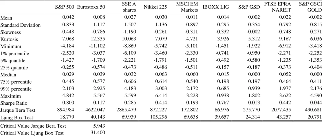
Regarding traditional assets, equity indices exhibit slightly positive mean returns with S&P 500 showing the highest average daily returns and the lowest standard deviation. As expected, corporate and government bonds indices have low mean returns and showcase the lowest standard deviation among all financial assets. Commodities depicted by S&P GSCI gold provide the worst reward to volatility with negative mean return and an annualized Sharpe ratio of -0.04. On the other hand, real estate exhibit promising performance with a favorable annualized Sharpe ratio of 0.44.

Meanwhile, in line with Chuen et Al. (2017), I find that cryptocurrencies outperform traditional financial assets in terms of average daily returns and have the highest standard deviation by far.

(15)

14

As can be noticed, the 1% and 99 % percentiles show that extreme price movements are more severe for cryptocurrencies than for traditional assets. Albeit, the higher magnitude of positive returns is emphasized for cryptocurrencies when compared with negative ones.

In the case of skewness and kurtosis, I find Ripple, Dash and Litecoin to be positively skewed, a significant characteristic rational investors look for. In contrast, Bitcoin, equities, bonds and real estate display a negative skewness that indicates a higher tail risk. Additionally, I find that all-time series are leptokurtic. Eurostoxx 50 and Shanghai stock exchange present high excess kurtosis but to a lesser extent than altcoins.

Apart from Bitcoin, cryptocurrencies have very high excess kurtosis as the market for altcoins is still developing.

Therefore, the Jarque-Bera test supports the latter findings by rejecting the normality for all assets at 1% significance level. All the conventional assets and cryptocurrencies are not normally distributed. Moreover, I conduct Ljung box test to check for serial correlation. Hence, I find most conventional assets as well as Ripple to show significant autocorrelation. Nevertheless, Bitcoin, Dash, S&P500, Sovereign bonds and Gold display a low autocorrelation of daily returns, which suggests a lack of predictability.

Cryptocurrencies pronounced deviation from normality is visualized in Figure 1. The black line depicts a theoretical normal distribution of Bitcoin. I observe that the latter is the least volatile with more observations around the mean and a less pronounced tail than altcoins.

5.2. Correlation analysis

Accurate correlation assessment is one fundamental aspect in portfolio theory. According to Corbet et Al. (2018), such important metric has momentous implications on portfolio construction, diversification and hedging.

(16)

15

Figure 2 illustrates pairwise correlation coefficients, which give a first snapshot of average correlations between our different financial assets. It is noteworthy that almost all correlation coefficients between cryptocurrencies and traditional assets do not exceed 0.10. Regarding cryptocurrencies, they range from 0.25 to 0.59 with Bitcoin and Litecoin exhibiting the highest correlation. Relatively, traditional assets have more varying correlations within themselves due to their global diversification. Yet, this is only the average correlation for our sample period. That is why I derive the multi-varying correlation through the Dynamic conditional correlation model.

Tables 4, 5, 6 and 7 illustrate descriptive statistics of dynamic conditional correlations between the innovations of each of the cryptocurrencies and traditional assets. The multi-varying correlation analysis will allow us to asses precisely the diversification and hedging benefits of cryptocurrencies.

Table 4 depicts the DCC statistics for correlation pairs within Bitcoin. The latter displays negative correlation among all the sample period with the following asset categories: developed corporate bonds, global real estate and Chinese equities. Hence, it acts as a strong hedge according to the definition of Baur and Lucey (2010). Moreover, it has a correlation of approximately zero with gold, MSCI emerging markets and sovereign bonds. It is also notable that the standard deviation of those correlation pairs is very low suggesting a stable correlation over time and high diversification benefits. Regarding developed market equities, Bitcoin is negatively correlated to Nikkei 225 on average with a maximum value of 0.0194.

The highest average correlation from all conventional assets is the pair with Eurostoxx 50 with a value of 0.0649. Nevertheless, it is very stable among all the period. For S&P 500, DCC correlation is more dynamic with a maximum spike of 0.27.

(17)

16

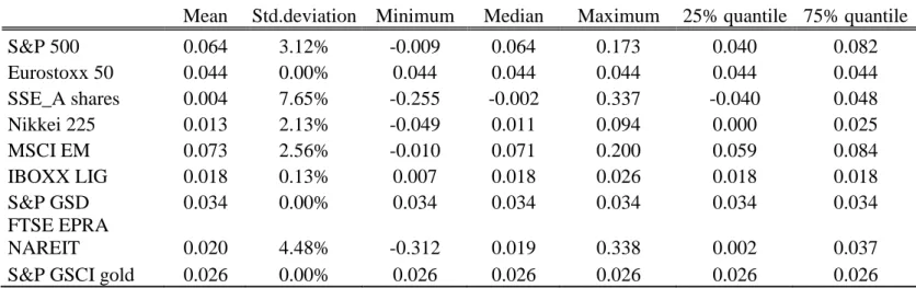
Table 5 reveals that Ripple cannot be regarded as a strong hedge against any of the traditional assets. A further look into the descriptive statistics of DCC correlations brings to light the noisy correlation spikes. Moreover, the 25% and 75% quantiles show slightly positive correlations with traditional assets over the whole sample period.

Table 6 shows that Dash has the highest correlation with developed market equities within all the cryptocurrencies. Furthermore, dynamic correlation is unstable for emerging markets equities and alternative investments since it swings from negative to positive. Yet, it can be considered as a strong hedge against developed corporate and sovereign bonds only.

According to table 7, Litecoin possesses hedging capacities against Japanese equities and global real estate. In addition, Low co-movements with equity market indices are more persistent than for Ripple and Dash which suggests better investment opportunities.

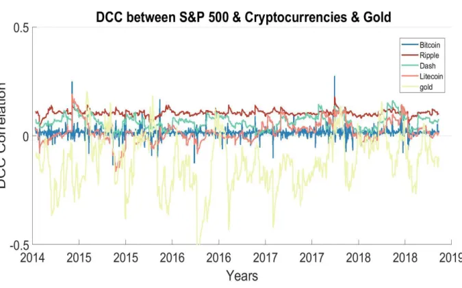
It is apparent that S&P 500 shows unstable dynamic correlations with cryptocurrencies all over the sample period. For a better assessment of hedging capacities, figure 2 plots its DCC correlation with cryptocurrencies as well as gold. The latter is added as a reference point since it is depicted as a safe haven against S&P 500. (Baur & Mc Dermott 2016).

Ripple and Dash show mostly positive correlations as already stated. Meanwhile, Bitcoin and Litecoin exhibit a wide range of positive and negative correlation values. Albeit, with small periods and no persistence while being negative. Gold, on the contrary, shows negative dynamic correlation for successive several months. In this regard, safe haven and strong hedge attributes should be excluded for Bitcoin and Litecoin. They can only be very effective diversifiers against S&P 500.

5.3. Portfolio performance

In this section, I discuss the results of the different optimization frameworks performed for the three optimal portfolios: a portfolio of traditional assets, a portfolio of traditional assets and

(18)

17

Bitcoin and finally, a portfolio of traditional assets, Bitcoin and the three alternative cryptocurrencies: Ripple, Dash and Litecoin.

Table 8 reports the performance of the optimal portfolios under the Minimum Variance optimization. I find that allocating Bitcoin to the basic portfolio slightly increases the annualized returns. Interestingly, the volatility of the optimal portfolio remains unchanged and maximum drawdown is even lower.

Likewise, the inclusion of alternative cryptocurrencies increases a bit more the returns but at the cost of a slightly higher volatility and a higher maximum drawdown. In fact, allocating even an insignificant share into altcoins does not compensate for their very high volatility. However, the higher returns seem to offset the evident increase in risk and the risk return reward of 1.26 vindicates the importance of adding Cryptocurrencies to the basic portfolio.

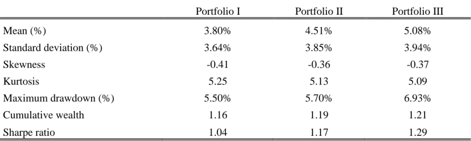
Due to the fat tail problem of cryptocurrencies, Conditional Value at Risk emerges as more coherent risk measure than variance. Table 9 presents the performance of Minimum Conditional Value at Risk optimization. It is important to note that the strategy’s ability to focus on the expected shortfall only brought higher returns for the portfolios with cryptocurrencies.

When including Bitcoin in the basic portfolio, the strategy shows a slight increase in the returns from 3.8% to 4.51%. The inclusion of alternative cryptocurrencies improved more the returns with an annualized mean of 5.08%. Once again, the high returns of cryptocurrencies offset their excess volatilities. Despite the increase in standard deviation, annualized Sharpe ratio increases from 1.05 to 1.17 when adding Bitcoin and to 1.29 when Altcoins are included.

Skewness and kurtosis of the second and third portfolios are slightly improved. Cumulative wealth increases as well. However, I observe a higher maximum drawdown when including Bitcoin and the effect is more prominent for the third portfolio.

(19)

18

Optimal portfolio weights is the main scope of the two aforementioned risk strategies. Now, I switch to risk budgeting strategies which impose constraints on the volatility contribution of each asset to the total portfolio volatility.

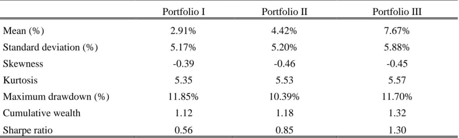
Table 10 summarizes the results of the inverse volatility strategy. I observe that diversification effects of this framework worsen off the performance of the basic portfolio. In fact, all the indices in the portfolio have positive weights in spite of their level of risk while the two first strategies omit weight allocations for the riskiest assets. The basic portfolio gives mean return of 2.9%, a standard deviation of 5.17% and a Sharpe ratio of only 0.56. The effect of cryptocurrencies is more prominent here. When adding Bitcoin, Sharpe ratio increased by 0.28 from 0.56 up to 0.85 that is driven by a significant improve in returns and an insignificant increase in volatility of 0.03%. The contribution of alternative cryptocurrencies is even more significant. Portfolio III displays a risk return efficiency of 1.30 and a cumulative wealth of 1.30. Contrariwise, maximum drawdown is again higher than first and second portfolios. Lastly, table 11 illustrates the performance of the maximum diversification strategy, which aims to maximize diversification effects by creating a portfolio with minimally correlated assets. Effective diversification benefits of cryptocurrencies are the most pronounced under this strategy. In fact, adding cryptocurrencies increases drastically the performance of the basic portfolio as Sharpe ratio increases from 0.73 to 1.22 with Bitcoin and up to 1.54 when adding Ripple, Dash and Litecoin. The strategy displays the highest returns for the second and third portfolio as well as the highest standard deviation. Once more, the skyrocket returns of cryptocurrencies seem to outweigh their high volatility.

Portfolio III shows higher maximum drawdown of 9.46% and more leptokurtic returns. However, it is important to pinpoint that this is the only portfolio to display positive skewness, which means that the probability of positive returns was higher than negative ones. Moreover, portfolio III hits the highest level of cumulative wealth with 1$ turning into 1.37$.

(20)

19

So far, this study revealed crucial portfolio benefits when adding cryptocurrencies to a traditional assets’ portfolio independently of the optimization strategy employed.

For further insights, a detailed analysis of portfolios weight allocation is presented in the following section.

5.4. Portfolio weights analysis

As can be seen from the asset allocation weights graphs, portfolios of traditional assets under inverse volatility and maximum diversification strategies are more diversified. On the other hand, Conditional Value at Risk strategy sets extreme weight allocations to bonds indices followed by S&P 500 since they exhibit the least volatility. Therefore, the C-var optimizer omits weighting other indices, which performed really bad and were highly volatile during estimation periods. This results in the basis portfolio exhibiting the best performance under this strategy with a Sharpe of 1.07.

When cryptocurrencies are included, I notice that the weighting scheme of other asset classes fluctuates to compensate for the additional volatility. Equity indices weights change the most during the sample period. I observe a significant increase in S&P 500 proportion but also a small position taken in gold. In addition, through the whole investment period, optimal portfolios contain between 0 and 3% of cryptocurrencies with the higher allocation share during the years 2016-2017, the period of tremendous growth for cryptocurrencies. Indeed, cryptocurrencies are considered too risky for the parameters of the optimization problem. It is also noticeable that Bitcoin dominates over alternative cryptocurrencies. In fact, none of the Altcoins is given more than 1% weight during the whole optimization process.

Regarding risk budgeting approaches, I observe that portfolio assets do not fluctuate that much when adding cryptocurrencies. Moreover, the weight allocated to cryptocurrencies is larger under those two strategies. Until 2017, there is an increasing allocation in cryptocurrencies. However, it decreases drastically after the Bitcoin boom.

(21)

20

Furthermore, the Maximum Diversification strategy, which boosted the performance of investments significantly, invests between 0 and 10% in cryptocurrencies. Thus, the higher cryptocurrency exposure had a huge impact on maximizing the portfolio performance.

5.5. Robustness check

To assess the robustness of the trading strategies results, tables 12, 13, 14 and 15 present performance results using weekly data and monthly rebalancing.

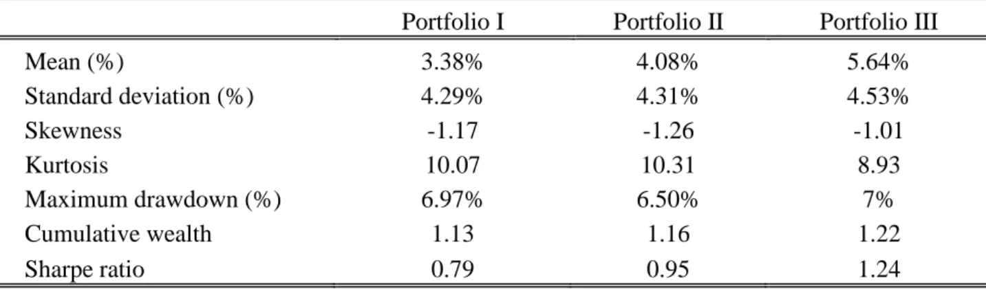
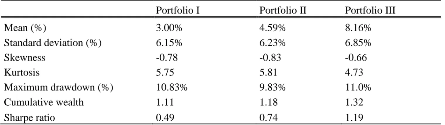
The results of the study are robust with regard to the asset allocations employed. I find that cryptocurrencies always add substantial value when included in the stocks-bonds-alternative investments portfolio. Sharpe ratio increases significantly under the different optimization frameworks. However, similar results regarding the downside risk of the basis portfolio are found when using weekly data. Alternative cryptocurrencies worsen of the maximum drawdown of the portfolio whereas Bitcoin increases slightly the maximum drawdown under Inverse volatility and minimum variance strategies.

Interestingly, Minimum conditional value at risk performs better than maximum diversification and yields the highest Sharpe Ratio when cryptocurrencies are added.

6. Conclusion

This study seeks to address the possible hedging and diversification benefits of cryptocurrencies as an alternative investment. From the perspective of a global investor, I investigate the market linkages between Cryptocurrencies and global asset indices as well as the benefits of their inclusion within these assets.

(22)

21

Using the dynamic conditional correlation model, I find that block-chain assets can act as effective diversifiers for the investment period analyzed. I also detect that the correlation of traditional assets against Bitcoin are closer to zero and more stable than against over crypto-tokens. Moreover, I find that Bitcoin, Dash and Litecoin do possess hedging properties against some assets’ indices. However, none of the cryptocurrencies acts as hedge against European, American and emerging market equities.

The resulting diversification properties further endorse the cryptocurrencies use case in a diversified portfolio. These findings are useful for global investors seeking protection from markets downward movements. I examine the out of sample performance of portfolios with and without cryptocurrencies via risk-based investment strategies: minimum variance, minimum conditional value at risk, inverse volatility and maximum diversification.

The results are in line with previous research regarding the inclusion of Bitcoin in a global portfolio of equities, bonds and alternative assets. I find that the risk return efficiency is enhanced under all strategies. The small increase in volatility was compensated with proportionally greater returns.

Despite their extreme volatility, the addition of alternative cryptocurrencies to a global diversified portfolio, which already contains Bitcoin, enhances the risk return reward. However, these crypto-assets yield higher volatility and higher maximum drawdown under all strategies. Further, the performance of the portfolio is boosted significantly under inverse volatility and maximum diversification. In fact, these modern risk based strategies prompt higher risk return reward via greater cryptocurrency exposure and especially greater alternative cryptos exposure. On the other side, due to their volatility structure, Minimum variance and Minimum C-var strategies invested in cryptocurrencies and particularly in Bitcoin only in certain points of time.

(23)

22

Moreover, the hedging properties of Cryptocurrencies are analyzed via the portfolios maximum drawdown. When adding Bitcoin, I find that it slightly drops under minimum variance and inverse volatility strategy. However, when Dash, Ripple and Litecoin are further added, the maximum drawdown increases under the four optimization models.

As robustness checking, I apply the aforementioned allocation strategies using weekly data. Results persist robustly. Cryptocurrencies enhance the portfolio performance on risk-adjusted basis but do not really decrease the portfolio downside risk.

In a nutshell, the study evidence suggests that cryptocurrencies can act as outstanding diversifier tools on a global perspective but do not offer appealing hedging properties.

However, the results of this study should be interpreted with caution. This analysis employs only limited asset allocation strategies. The sample period is small due to the short history of cryptocurrencies and better alternative to the selected cryptocurrencies might exist.

(24)

23 Appendix:

Table 1: Descriptive statistics of traditional assets.

Summary statistics of daily log returns for traditional assets from 31 July 2014 to 30 April 2019. (N=1238 observations). Results are reported on a percentage basis apart from skewness, kurtosis, Sharpe ratio, the JB and LJBox tests. In addition, Sharpe ratio is annualized.

S&P 500 Eurostoxx 50 SSE A

shares Nikkei 225

MSCI EM

Markets IBOXX LIG S&P GSD

FTSE EPRA NAREIT S&P GSCI GOLD Mean 0.042 0.008 0.027 0.030 0.011 0.014 0.002 0.022 -0.002 Standard Deviation 0.833 1.117 1.507 1.136 0.897 0.295 0.354 0.792 0.815 Skewness -0.448 -0.786 -1.190 -0.261 -0.311 -0.332 -0.002 -0.748 0.271 Kurtosis 7.068 12.335 10.063 7.079 4.721 3.926 5.312 9.167 6.036 Minimum -4.184 -11.102 -8.869 -5.742 -5.101 -1.451 -1.922 -6.912 -3.418 1% percentile -2.520 -3.037 -6.109 -3.460 -2.330 -0.741 -0.950 -2.271 -2.252 5% quantile -1.427 -1.709 -2.221 -1.791 -1.501 -0.492 -0.580 -1.235 -1.353 25% quantile -0.255 -0.574 -0.473 -0.486 -0.511 -0.157 -0.187 -0.373 -0.404 Median 0.029 0.039 0.032 0.063 0.060 0.015 0.000 0.052 0.000 75% percentile 0.445 0.577 0.606 0.614 0.540 0.198 0.197 0.464 0.411 99% percentile 2.103 2.925 4.183 3.003 2.172 0.685 0.939 1.977 2.176 Maximim 4.842 5.567 5.599 6.414 3.228 0.938 1.802 3.622 4.590 Sharpe Ratio 0.800 0.117 0.285 0.414 0.193 0.767 0.013 0.442 -0.044

Jarque Bera Test 894.984 4622.047 2865.479 872.227 172.802 66.976 275.770 2077.435 490.681

Ljung Box Test 18.779 40.143 69.939 105.296 69.638 39.657 24.314 43.257 20.791

Critical Value Jarque Bera Test 5.943

(25)

24 Table 2: Descriptive statistics of cryptocurrencies.

Summary statistics of daily log returns for cryptocurrencies from 31 July 2014 to 30 April 2019. (N=1238 observations).

Bitcoin Ripple Dash Litecoin

Mean 0.179 0.330 0.242 0.185 Standard Deviation 4.394 7.513 7.522 6.945 Skewness -0.210 2.381 0.015 1.000 Kurtosis 8.206 20.257 27.050 15.789 Minimum -23.874 -35.328 -86.020 -51.393 1% percentile -13.533 -18.051 -19.343 -15.550 5% quantile -7.056 -9.364 -9.759 -8.994 25% quantile -1.423 -2.430 -2.845 -2.138 Median 0.222 -0.345 -0.276 0.000 75% percentile 1.890 2.089 2.990 1.822 99% percentile 13.828 27.293 23.589 26.831 Maximim 22.512 75.083 76.818 53.980 Sharpe Ratio 0.645 0.698 0.511 0.422

Jarque Bera Test 1406.84 16530.00 29834.76 8643.49

Ljung Box Test 31.76 91.30 26.56 36.60

Critical Value Jarque Bera Test 5.94

(26)

25 Table 3: Correlation matrix

This table shows unconditional pairwise correlation coefficients between cryptocurrencies and traditional assets from 31 July 2014 to 30 April 2019.

Bitcoin Ripple Dash Litecoin S&P500 Eurostoxx 50 SSE A Shares Nikkei 225 MSCI EM IBOXX LIG S&P GSD FTSE EPRA S&P GSCI GOLD Bitcoin 1.000 0.330 0.485 0.592 0.039 0.036 0.012 -0.037 0.016 -0.023 0.010 -0.019 0.023 Ripple 1.000 0.254 0.332 0.053 0.030 -0.007 0.020 0.063 0.035 0.033 0.010 0.026 Dash 1.000 0.431 0.080 0.068 0.030 -0.013 0.049 -0.073 -0.037 -0.017 -0.006 Litecoin 1.000 0.026 0.004 -0.015 -0.026 0.007 -0.006 0.009 -0.015 -0.016 S&P500 1.000 0.493 0.162 0.065 0.441 -0.193 -0.214 0.515 -0.138 Eurostoxx 50 1.000 0.127 0.160 0.578 -0.125 -0.026 0.256 -0.099 SSE A Shares 1.000 0.211 0.413 0.013 -0.101 0.230 -0.058 Nikkei 225 1.000 0.416 0.203 0.124 0.181 0.102 MSCI EM 1.000 0.022 -0.032 0.435 0.018 IBOXX LIG 1.000 0.446 0.108 0.280 S&P GSD 1.000 -0.373 0.558 FTSE EPRA NAREIT 1.000 -0.177 S&P GSCI GOLD 1.000

(27)

26

The subsequent tables summarize the dynamic conditional correlations between daily returns of the four cryptocurrencies and traditional asset class. Standard deviations are expressed in percentage.

Table 4: DCC statistics for traditional assets against Bitcoin

Mean Std.deviation Minimum Median Maximum

25% quantile 75% quantile S&P 500 0.0146 2.2501% -0.1343 0.0147 0.2738 0.0099 0.0194 Eurostoxx 50 0.0648 0.0022% 0.0648 0.0648 0.0649 0.0648 0.0648 SSE_A shares -0.0056 0.0038% -0.0061 -0.0056 -0.0052 -0.0056 -0.0056 Nikkei 225 -0.0374 3.2494% -0.0977 -0.0317 0.0194 -0.0693 -0.0102 MSCI EM 0.0196 0.0002% 0.0196 0.0196 0.0196 0.0196 0.0196 IBOXX LIG -0.0149 0.0002% -0.0150 -0.0149 -0.0149 -0.0149 -0.0149 S&P GSD 0.0112 0.2561% -0.0252 0.0112 0.0243 0.0106 0.0118 FTSE EPRA NAREIT -0.0320 0.2980% -0.0541 -0.0321 -0.0029 -0.0331 -0.0310

S&P GSCI gold 0.0166 0.0002% 0.0165 0.0166 0.0166 0.0166 0.0166

Figure 1 : Density of Cryptocurrencies.

The following figure illustrates Gaussian kernel density estimators of cryptocurrencies against fitted normal distribution.

(28)

27 Table 6: DCC statistics for traditional assets against DASH.

Table 5: DCC statistics for traditional assets against Ripple

Mean Std.deviation Minimum Median Maximum 25% quantile 75% quantile

S&P 500 0.064 3.12% -0.009 0.064 0.173 0.040 0.082 Eurostoxx 50 0.044 0.00% 0.044 0.044 0.044 0.044 0.044 SSE_A shares 0.004 7.65% -0.255 -0.002 0.337 -0.040 0.048 Nikkei 225 0.013 2.13% -0.049 0.011 0.094 0.000 0.025 MSCI EM 0.073 2.56% -0.010 0.071 0.200 0.059 0.084 IBOXX LIG 0.018 0.13% 0.007 0.018 0.026 0.018 0.018 S&P GSD 0.034 0.00% 0.034 0.034 0.034 0.034 0.034 FTSE EPRA NAREIT 0.020 4.48% -0.312 0.019 0.338 0.002 0.037

S&P GSCI gold 0.026 0.00% 0.026 0.026 0.026 0.026 0.026

S&P 500 0.11 1.4% 0.03 0.10 0.18 0.10 0.11 Eurostoxx 50 0.10 3.1% -0.08 0.10 0.27 0.09 0.11 SSE_A shares 0.04 0.0% 0.04 0.04 0.04 0.04 0.04 Nikkei 225 0.02 0.7% -0.03 0.02 0.11 0.02 0.03 MSCI EM 0.08 2.5% 0.00 0.08 0.18 0.07 0.10 IBOXX LIG -0.07 0.0% -0.07 -0.07 -0.07 -0.07 -0.07 S&P GSD -0.04 0.0% -0.04 -0.04 -0.04 -0.04 -0.04 FTSE EPRA NAREIT -0.01 8.2% -0.45 -0.01 0.49 -0.05 0.03

(29)

28

S&P 500 0.018 4.89% -0.164 0.011 0.192 -0.010 0.040 Eurostoxx 50 0.035 1.88% -0.036 0.035 0.120 0.027 0.043 SSE_A shares -0.027 2.90% -0.099 -0.029 0.042 -0.044 -0.014 Nikkei 225 -0.021 0.00% -0.021 -0.021 -0.021 -0.021 -0.021 MSCI EM 0.020 2.47% -0.086 0.020 0.110 0.006 0.033 IBOXX LIG -0.010 4.31% -0.129 -0.009 0.181 -0.031 0.012 S&P GSD 0.001 0.00% 0.001 0.001 0.001 0.001 0.001 FTSE EPRA NAREIT -0.016 0.00% -0.017 -0.016 -0.016 -0.016 -0.016

S&P GSCI gold -0.016 5.46% -0.207 -0.009 0.154 -0.046 0.018

Table 7: DCC statistics for traditional assets against Litecoin

(30)

29

The following tables present the performance of the three optimal portfolios: Portfolio I: a portfolio of traditional assets, which encompasses equities, bonds and alternative investments. Portfolio II: a portfolio of traditional assets and Bitcoin. Portfolio III: a portfolio of traditional assets, Bitcoin and alternative cryptocurrencies. Four different optimization frameworks are performed subsequently: Minimum variance, Minimum Conditional Value at Risk, Inverse Volatility and Maximum Diversification frameworks. I use a 200 days moving window and the out of sample period ranges from May-08-2015 to April-30-2019. Sharpe ratio, mean daily return and standard deviation are annualized.

Table 8: Minimum Variance strategy

Table 9: Minimum conditional value at risk strategy

Portfolio I Portfolio II Portfolio III

Mean (%) 3.81% 4.14% 4.60% Standard deviation (%) 3.62% 3.62% 3.64% Skewness -0.45 -0.44 -0.43 Kurtosis 5.30 5.24 5.06 Maximum drawdown (%) 5.43% 5.37% 5.45% Cumulative wealth 1.16 1.17 1.19 Sharpe ratio 1.05 1.14 1.26

(31)

30 Table 10 : Inverse volatility strategy.

Table 11 : Maximum diversification strategy.

Mean (%) 3.31% 5.94% 8.75% Standard deviation (%) 4.50% 4.86% 5.65% Skewness -0.37 -0.31 0.07 Kurtosis 5.08 4.91 7.09 Maximum drawdown (%) 8.15% 9.40% 9.46% Cumulative wealth 1.13 1.24 1.36 Sharpe ratio 0.73 1.22 1.54

(32)

31 FIGURES: Weight Allocation

The following graphs display the weight allocation for traditional assets and cryptocurrencies from 8 May 2015 until 30 April 2019 under the following strategies: minimum conditional value at risk, inverse volatility, and maximum diversification.

0,00 0,10 0,20 0,30 0,40 0,50 0,60 0,70 0,80 0,90 1,00 08.05.2015 08.07.2015 08.09.2015 08.11.2015 08.01.2016 08.03.2016 08.05.2016 08.07.2016 08.09.2016 08.11.2016 08.01.2017 08.03.2017 08.05.2017 08.07.2017 08.09.2017 08.11.2017 08.01.2018 08.03.2018 08.05.2018 08.07.2018 08.09.2018 08.11.2018 08.01.2019 08.03.2019 We ig h ts Year

Minimum Conditional Value at Risk Portfolio of traditional assets

S&P 500 Eurostoxx 50 SSE A Shares Nikkei 225 MSCI EM

IBOXX LIG S&P GSD FTSE EPRA NAREIT S&P GSCI GOLD

0,00 0,10 0,20 0,30 0,40 0,50 0,60 0,70 0,80 0,90 1,00 08.05.2015 08.07.2015 08.09.2015 08.11.2015 08.01.2016 08.03.2016 08.05.2016 08.07.2 01 6 08.09.2016 08.11.2016 08.01.2017 08.03.2017 08.05.2017 08.07.2017 08.09.2017 08.11.2017 08.01.2018 08.03.2018 08.05.2018 08.07.2018 08.09.2018 08.11.2 01 8 08.01.2019 08.03.2019 W e ig h ts Year

Minimum Conditional Value at Risk

Portfolio of tradtional assets and cryptocurrencies

Bitcoin Ripple Dash Litecoin S&P500

Eurostoxx 50 SSE A Shares Nikkei 225 MSCI EM IBOXX LIG

(33)

32 0,00 0,10 0,20 0,30 0,40 0,50 0,60 0,70 0,80 0,90 1,00 08.05.2015 08.07.2015 08.09.2 01 5 08.11.2015 08.01.2016 08.03.2016 08.05.2016 08.07.2016 08.09.2016 08.11.2016 08.01.2017 08.03.2 01 7 08.05.2017 08.07.2017 08.09.2017 08.11.2017 08.01.2018 08.03.2018 08.05.2018 08.07.2018 08.09.2018 08.11.2018 08.01.2019 08.03.2019 We ig h ts Year Inverse Volatility

Portfolio of traditional assets and cryptocurrencies

S&P GSD FTSE EPRA NAREIT S&P GSCI GOLD

0,00 0,10 0,20 0,30 0,40 0,50 0,60 0,70 0,80 0,90 1,00 08.05.2015 08.07.2015 08.09.2015 08.11.2015 08.01.2016 08.03.2016 08.05.2016 08.07.2 01 6 08.09.2016 08.11.2016 08.01.2017 08.03.2017 08.05.2017 08.07.2017 08.09.2017 08.11.2017 08.01.2018 08.03.2018 08.05.2018 08.07.2018 08.09.2018 08.11.2 01 8 08.01.2019 08.03.2019 We ig h ts Year Inverse Volatility Portfolio of traditional assets

S&P 500 Eurostoxx 50 SSE A Shares Nikkei 225 MSCI EM

(34)

33 0,00 0,10 0,20 0,30 0,40 0,50 0,60 0,70 0,80 0,90 1,00 08.05.2015 08.07.2015 08.09.2015 08.11.2015 08.01.2016 08.03.2016 08.05.2016 08.07.2 01 6 08.09.2016 08.11.2016 08.01.2017 08.03.2017 08.05.2017 08.07.2017 08.09.2017 08.11.2017 08.01.2018 08.03.2018 08.05.2018 08.07.2018 08.09.2018 08.11.2 01 8 08.01.2019 08.03.2019 We ig h ts Year Maximum Diversification Portfolio of traditional assets

S&P 500 Eurostoxx 50 SSE A shares Nikkei 225 MSCI EM

IBOXX LIG S&P GSD FTSE EPRA NAREIT S&P GSCI GOLD

0,00 0,10 0,20 0,30 0,40 0,50 0,60 0,70 0,80 0,90 1,00 08.05.2015 08.07.2015 08.09.2015 08.11.2015 08.01.2016 08.03.2016 08.05.2016 08.07.2 01 6 08.09.2016 08.11.2016 08.01.2017 08.03.2017 08.05.2017 08.07.2017 08.09.2017 08.11.2017 08.01.2018 08.03.2018 08.05.2018 08.07.2018 08.09.2018 08.11.2 01 8 08.01.2019 08.03.2019 We ig h ts Year Maximum Diversification

Portfolio of traditional assets and crytocurrencies

(35)

34

The subsequent tables present the results obtained from the robustness check. It reports the performance of the optimal portfolios when using weekly data. I use 40 weeks (Equivalent of 200 trading days) moving window and the out of sample period ranges from May-08-2015 to April-30-2019. Sharpe ratio, mean daily return and standard deviation are annualized.

Table 12: Minimum variance strategy

Table 13: Minimum conditional value at risk strategy

Mean (%) 3.38% 4.08% 5.64% Standard deviation (%) 4.29% 4.31% 4.53% Skewness -1.17 -1.26 -1.01 Kurtosis 10.07 10.31 8.93 Maximum drawdown (%) 6.97% 6.50% 7% Cumulative wealth 1.13 1.16 1.22 Sharpe ratio 0.79 0.95 1.24

(36)

35 Table 14: Inverse volatility strategy

Table 15: Maximum diversification strategy

Mean (%) 3.11% 6.55% 11.64% Standard deviation (%) 5.76% 6.52% 8.83% Skewness -1.24 -1.20 0.36 Kurtosis 9.39 8.25 7.40 Maximum drawdown (%) 8.69% 10.02% 9.57% Cumulative wealth 1.12 1.26 1.45 Sharpe ratio 0.54 1.00 1.31

(37)

Salma Ouali

36 References

Bouri, E., Molnár, P., Azzi, G., Roubaud, D., Hagfors, L.I., 2017. On the hedge and safe haven properties of Bitcoin: Is it really more than a diversifier? Finance Research Letters 20, 192-198. Briere, M., Oosterlinck, K., Szafrz, A., 2015. Virtual currency, tangible return: Portfolio diversification with bitcoin. Journal of Asset Management, 16, 6, 365-373.

Brauneis, A., Mestel, R., 2019. Cryptocurrency-portfolios in a mean-variance framework. Finance Research Letters 28, 259-264.

Dyhrberg, A. H., 2016. Bitcoin, gold and the dollar- A GARCH volatility analysis. Finance Research Letters, 85-92.

Eisl, A., Gasser, S.M., Weinmayer, K., 2015. Caveat emptor: Does bitcoin improve portfolio diversification?

Engle, E., 2000. Dynamic conditional correlation – A simple class of multivariate GARCH models.

Guesmi, K. Samir Saadi, S., Abid, I., Ftiti, Z., 2018. Portfolio diversification with virtual currency: Evidence from bitcoin. International Review of Financial Analysis.

Henriques, I., Sadorsky, P., 2018. Can bitcoin replace gold in an investment portfolio? Journal of Risk and Financial Management 11, 48.

Hong, K., 2016. Bitcoin as an alternative investment vehicle. Springer Science+ Business Media

Kajtazi, A., Moro, A., 2017. Bitcoin, portfolio diversification and Chinese financial markets

Klein, T., Thu, H.P., Walthe, T., 2018. Bitcoin is not the new gold, a comparison of volatility, correlation, and portfolio performance. Working paper.

Lee, D.K.K., Li Guo, L., Yu Wang, Y., 2017. Cryptocurrency: A new investment opportunity? Liu, W., 2018. Portfolio diversification across cryptocurrencies. Finance Research Letters. Lorenz, J., Strika, M., 2017. Bitcoin and cryptocurrencies - not for the faint-hearted. International Finance and Banking 4, 1.

Petukhina, A., Trimborn, S., Härdle, W.K., Elendner, H., 2018. Investing with cryptocurrencies – evaluating the potential of portfolio allocation.

Platanakis, E., Urquhart, A., 2018. Should investors include bitcoin in their portfolios? A portfolio theory approach.

Rockafellar, R.T., Uryasev, S., 1999. Optimization of conditional value at risk. Journal of Risk, 21-41.

(38)

Salma Ouali

37

Svärd, S., 2014. Dynamic portfolio strategy using multivariate garch model. Working Paper Symitsi, E., Chalvatzis, K.J., 2019. The economic value of bitcoin: A portfolio analysis of currencies, gold, oil and stocks. Research in International Business and Finance 48, 97-110. Urquhart, A., Zhang, H., 2016. Bitcoin a hedge or safe-haven for currencies? An intraday analysis.