Real and complex hedgehogs of C
n+1
,
their symplectic area, curvature and evolutes
Yves Martinez-Maure
[email protected]
Abstract
Classical (real) hedgehogs can be regarded as the geometrical realiza-tions of formal di¤erences of convex bodies in Rn+1. Like convex bodies,
hedgehogs can be identi…ed with their support functions. Adopting a pro-jective viewpoint, we prove that any holomorphic function h : Cn
! C can be regarded as the ‘support function’ of a complex hedgehog Hhin
Cn+1. In the same vein, we introduce the notion of evolute of such a hedgehog Hh in C2, and a natural (but apparently hitherto unknown)
notion of complex curvature, which allows us to interpret this evolute as the locus of the centers of complex curvature. It is of course permissible to think that the development of a ‘Brunn-Minkowski theory for complex hedgehogs’ (replacing Euclidean volumes by symplectic ones) might be a promising way of research. We give …rst two results in this direction. We next return to real hedgehogs in R2n endowed with a linear complex
structure. We introduce and study the notion of evolute of a hedgehog. We particularly focus our attention on R4 endowed with a linear Kähler structure determined by the datum of a pure unit quaternion. In parallel, we study the symplectic area of the images of the oriented Hopf circles under hedgehog parametrizations and introduce a quaternionic curvature function for such an image. Finally, we consider brie‡y the convolution of hedgehogs, and the particular case of hedgehogs in R4n regarded as a
hyperkähler vector space.
Contents:
1. Introduction and statement of main results 2. Background on classical real hedgehogs
3. Complex hedgehogs in Cn+1 or Pn+1(C)
3.1. Real and complex hedgehogs as dual hypersurfaces of graphs
0
2010 MSC:
Key words and phrases: Real and complex hedgehogs, Brunn-Minkowski theory, mixed sym-plectic areas, evolutes, rational curves, complex or quaternionic curvature function, linear complex structure, Kähler vector spaces
3.2. Complex hedgehogs as fronts in Cn+1 of Legendrian immersions in C2n+1
3.3. Rational hedgehogs of the complex projective plane P2(C)
3.4. Evolute of a plane complex hedgehog as locus of its centers of curvature
3.5 Real and imaginary parts of Hh C2 regarded as hedgehogs of R3
4. Towards a Brunn-Minkowski theory for complex hedgehogs 4.1. Mixed symplectic area
4.2. A sharp estimation of the area using the energy
5. Real hedgehogs in Cn=R2n and their evolutes
5.1. Evolutes of hedgehogs hypersurfaces in R4
5.2. Symplectic and mixed symplectic area 5.3. Quaternionic curvature function 5.4. Convolution of hedgehogs
5.5. Evolutes of hedgehogs hypersurfaces in Hn=R4n
1
Introduction and statement of main results
Classical (real) hedgehogs can be regarded as the geometrical realizations of
formal di¤erences of convex bodies in the Euclidean vector space Rn+1. The
idea of considering the Minkowski di¤erences of convex bodies may be traced back to some papers by A.D. Alexandrov [1] and H. Geppert [4] in the 1930’s. Many notions extend to hedgehogs and quite a number of classical results …nd their counterparts. Of course, a few adaptations are necessary. In particular, volumes have to be replaced by their algebraic versions. Hedgehogs have proved useful for studying convex bodies (one of the main successes of the theory is the construction of counterexamples to an old conjectured characterization of the 2-sphere [11, 15]), and for geometrizing analytical problems by considering functions as support functions. Section 2 will provide the reader with the nec-essary background on hedgehogs in order to facilitate an understanding of the following sections.
Complex hedgehogs
Like convex bodies of Rn+1, hedgehogs of Rn+1are completely determined
by (and can be identi…ed with) their support functions, which are di¤erences of two support functions of convex bodies of Rn+1restricted to the unit sphere Sn. In section 3, we adopt a projective viewpoint in order to prove that:
Theorem. Any holomorphic function h : Cn ! C can be regarded as the
‘com-plex support function’ of a ‘com‘com-plex hedgehog’ Hh, which is de…ned by a
holo-morphic parametrization xh: Cn! Cn+1in the complex Euclidean space Cn+1.
Of course, these complex hedgehogs can be interpreted in the metric contact
geometry setting where they appear as fronts of Legendrian immersions in C2n+1
(see Subsection 3.2).
In passing, we introduce the notion of a rational hedgehog in the complex
(for an introduction to the Fubini-Study structure, see e.g. [2]). Such a hedgehog
Hh is modeled on P1(C) := C [ f1g via a holomorphic map h : C ! C that
is such that Area [xh(C)] < +1.
Complex evolutes and complex curvature
In classical di¤erential geometry of curves, the evolute of a plane curve is the locus of all its centers of curvature or, equivalently, the envelope of its normal lines. Interpreting evolutes of hedgehog curves from a projective point of view, we prove in Subsection 3.4 that:
Theorem. There exists a natural extension of the notion of evolute
curves to complex hedgehog curves, and a very natural (but appar-ently hitherto unknown) notion of complex curvature, which allows us
to interpret any evolute of a complex hedgehog curve Hh as the locus of its
centers of complex curvature.
Given any complex hedgehog Hhin R4, we introduce its real and imaginary
parts as hedgehogs of R3, which can be regarded globally as the images of H
h
under the orthogonal projections onto two particular hyperplanes of R4, and
that are determined by Re [h] and Im [h].
Towards a Brunn-Minkowski theory for complex hedgehogs
The notion of a hedgehog curve or surface was born in the thirties from the study of the Brunn-Minkowski theory by A.D. Aleksandrov, H. Geppert and some others. In the present paper, we try to motivate the development of a ‘theory of mixed volumes for complex hedgehogs’ (replacing Euclidean volumes by symplectic ones).
In Section 4, we mention …rst two results in this direction. First, identifying complex hedgehogs with their support functions, we notice that the complex linear space of holomorphic functions de…ned up to a similitude on the unit disc
D C can be endowed with a scalar product which can be interpreted as a mixed
symplectic area.
Second, we give the following sharp estimation of the (symplectic) area of
xh(D) using the energy, say E (xh) ; of the loop xh : S1 = R=2 Z ! C2,
7! xh ei , in the case where h : D ! C is the sum of a power series Phnzn
with radius of convergence R > 1: Area [xh(D)]
3
4E (xh) .
Note that this estimate is better than that well-known for an arbitrary smooth
loop : S1 ! V in a symplectic vector space (V; !) (namely, jA ( )j E ( ),
see for instance [14, pp. 87-88]). Real evolutes in even dimensions
In Section 5, we return to real hedgehogs but in R2n endowed with a linear
complex structure J . First of all, we introduce the notion of evolute of any
We particularly focus our attention on the case n = 2. We identify R4 with the quaternion algebra H (and thus the unit sphere S3to the set S1Hof unit
quaternions), and, we associate to any pure unit quaternion v the linear complex structure Jv: R4! R4, x 7 ! vx. In other words, for any v 2 S2=S1H\Im (H),
we choose to work in the Kähler vector space R4; J
v; !v , where !vdenotes the
associated Kähler form (i.e. the alternating 2-form !v(X; Y ) = hJvX; Y i, where
h:; :i is the standard Euclidean metric on R4 . To any v 2 S2, it thus corresponds
a Hopf …bration and a Hopf ‡ow leaving the Hopf …bration invariant, namely
the Hopf ‡ow f( v) g 2S1 given by ( v) (u) := (cos ) u + (sin ) vu, u 2 S3 .
We give a detailed study of evolutes of hedgehog hypersurfaces in these Kähler vector spaces R4; J
v; !v .
Mixed symplectic area and quaternionic curvature function
In parallel, we study the symplectic area of images of the oriented Hopf circles
under the hedgehog parametrizations xh : S3 ! R4; Jv; !v . In this setting,
we introduce the notion of mixed symplectic area and prove what follows among other results.
Theorem. Let h 2 C1 S3; R , and let v be a pure unit quaternion.
(i) The evolute of Hh in R4; Jv; !v is the hedgehog with support function
@vh : S3! R, u 7 ! hrh ( Jv(u)) ; ui ,
where h:; :i is the standard Euclidean metric on R4, and rh the gradient of h.
Thus, @vh is such that: 8u 2 S3,
(@vh) (Jv(u)) = hrh (u) ; Jv(u)i = (dh)u(Jv(u)) ;
(ii) For all u 2 S3,
x@vh(u) = xh(u) Rh(u; v) u,
where Rh(u; v):= vTuxh(Jv(u)) u ; here u of course refers to the quaternion
conjugate of u ;
(iii) The map Rh(:; v) : u := (cos ) u + (sin ) vu 7 ! Rh(u ; v) can be
in-terpreted as a quaternionic curvature function of xh S1u;v , where S1u;v is the
unit circle of C (u; v) := Ru + RJv(u) oriented by (u; Jv(u)), in the sense that
Rh(:; v) is the unique C1-smooth quaternionic function R (:; v) : S1u;v! H that
is of the form R (u ; v) = vTu (v), where Tu (v) is a pure quaternion, and
such that : 8g 2 C1 S3; R , su;v(g; h) := 1 2 Z 2 0 hx g(u ) ; R (u ; v) u i d ,
where su;v(g; h) denotes the mixed symplectic area of xg S1u;v and xh S1u;v .
In other words, what is shown by (iii) is that the quaternionic curvature
role as the (ordinary) curvature function of plane hedgehogs does relatively to the (ordinary) mixed area. Here, we have to recall that the mixed area of two
plane hedgehogs with support functions (g; h) 2 C1 S1; R 2is given by
a (g; h) := 1 2 Z 2 0 hx g(u ) ; Rh(u) u i d = 1 2 Z 2 0 g (u ) Rh(u ) d ,
where u = ei 2 C = R2, and where x
g : S1 ! C, 7! g ( ) u + g0( ) iu
the natural parametrization of Hg, and Rh := h + h00 the so-called ‘curvature
function’of Hh (see [9, p. 447]).
Relationship with the area of order 2
We also show that the algebraic area of order 2 of a hedgehog Hh of R4
can be interpreted in terms of the symplectic areas of Hh in the Kähler vector
spaces R4; J
v; !v . Here, we have to recall that the algebraic area of order 2 of
Hh is de…ned to be V (h; h; 1; 1), where V is the extension of the mixed volume
(of convex bodies of R4) to hedgehogs of R4.
Convolution and extension to R4n =Hn
Finally, we consider brie‡y the convolution of hedgehogs in Rn, and evolutes
of hedgehog hypersurfaces in R4n, which we identify with the hyperkähler vector
space (Hn; h:; :i ; I; J; K), where h:; :i is the standard Euclidean metric on R4n,
(n 1), and, the triple of complex structures (I; J; K) on Hn is given by left
multiplication by i; j; k respectively.
2
Background on classical real hedgehogs
In this section, we recall for the convenience of the reader the background on
real hedgehogs. The set Kn+1of all convex bodies of (n + 1)-Euclidean vector
space Rn+1is usually equipped with Minkowski addition and multiplication by
nonnegative real numbers, which are respectively de…ned by:
(i) 8(K; L) 2 Kn+1 2, K + L = fx + y jx 2 K; y 2 L g ;
(ii) 8 2 R+; 8K 2 Kn+1, :K = f x jx 2 K g .
It does not constitute a vector space since there is no subtraction in Kn+1:
not for every pair (K; L) 2 Kn+1 2 does there exist an X 2 Kn+1 such that
L + X = K. Now, in the same way as we construct the group Z; of integers from the monoid N of nonnegative integers, we can construct the vector space
Hn+1 of formal di¤erences of convex bodies from Kn+1. We can then regard
Kn+1 as a cone of Hn+1 that spans the entire space. Hedgehog theory simply
consists in:
1. considering each formal di¤erence of convex bodies of Rn+1as a geometrical
2. extending the mixed volume V : Kn+1 n+1 ! R to a symmetric (n +
1)-linear form on Hn+1;
3. extending certain parts of the Brunn-Minkowski theory to Hn+1.
For n 2, it goes back to a paper by H. Geppert [4] who introduced
hedge-hogs under the German names stützbare Bereiche (n = 1) and stützbare Flächen (n = 2).
C2 case. Here we follow more or less [8]. As is well-known, every convex
body K Rn+1 is determined by its support function h
K : Sn ! R, where
hK(u) is de…ned by hK(u) = sup fhx; ui jx 2 K g, (u 2 Sn), that is, as the signed
distance from the origin to the support hyperplane with normal vector u. In
particular, every closed convex hypersurface of class C2
+ (i.e., C2-hypersurface
with positive Gaussian curvature) is determined by its support function h (which
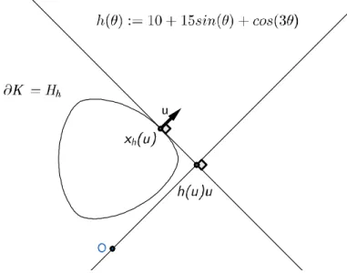
must be of class C2 on Sn [16, p. 111]) as the envelope Hh of the family
of hyperplanes with equation hx; ui = h(u). This envelope Hh is described
analytically by the following system of equations hx; ui = h(u) hx; : i = dhu(:)
.
The second equation is obtained from the …rst by performing a partial di¤eren-tiation with respect to u. From the …rst equation, the orthogonal projection of x onto the line spanned by u is h (u) u, and from the second one, the orthogonal
projection of x onto u? is the gradient of h at u (see Figure 1). Therefore,
for each u 2 Sn, x
h(u) = h(u)u + (rh) (u) is the unique solution of this system.
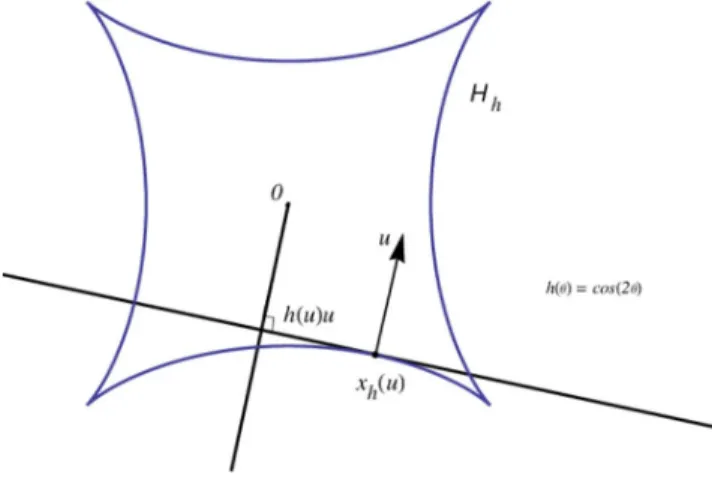
Now, for any C2-function h on Sn, the envelope Hh is in fact well-de…ned
(even if h is not the support function of a convex hypersurface). Its natural
parametrization xh : Sn ! Hh; u 7! h(u)u + (rh) (u) can be interpreted as
the inverse of its Gauss map, in the sense that: at each regular point xh(u) of
Hh, u is a normal vector to Hh. We say that Hhis the hedgehog with support
function h (see Figure 2). Note that xh depends linearly on h.
Since the parametrization xh can be regarded as the inverse of the Gauss
map, the Gaussian curvature Khof Hhat xh(u) is given by Kh(u) = 1=det[Tuxh],
where Tuxhis the tangent map of xhat u. Therefore, singularities are the very
points at which the Gaussian curvature is in…nite. For every u 2 Sn, the
tan-gent map of xh at the point u is Tuxh = h(u) IdTuSn+ Hh(u), where Hh(u)
is the symmetric endomorphism associated with the Hessian r2h u of h at u.
In particular, the so-called ‘curvature function’Rh(u) := det [Tuxh] is given by
Rh(u) = det [h(u) IdTuSn+ Hh(u)] for all u 2 S
n.
Figure 2. Plane hedgehog withC2-support
function
In computations, it is often more convenient to replace h by its positively
1 homogeneous extension to Rn+1n f0g, which is given by
' (x) := kxk h x
kxk ,
for x 2 Rn+1nf0g, where k:k is the Euclidean norm on Rn+1. A straightforward
computation gives:
(i) xhis the restriction of the Euclidean gradient of ' to the unit sphere Sn;
(ii) For all u 2 Sn, the tangent map Tuxh identi…es with the symmetric
endomorphism associated with the Hessian of ' at u.
Hedgehogs with a C2-support function can be regarded as Minkowski
all large enough real constant r, the functions h + r and r are support functions
of convex hypersurfaces of class C+2 such that h = (h + r) r.
General case. In [12], the author extended the notion of a hedgehog by
regarding hedgehogs as Minkowski di¤erences of arbitrary convex bodies. The trick is to de…ne hedgehogs inductively as collections of lower-dimensional ‘sup-port hedgehogs’. More precisely, the de…nition of general hedgehogs is based on the three following remarks.
(i) In R, every convex body K is determined by its support function hK as the
segment [ hK( 1) ; hK(1)], where hK( 1) hK(1), so that the di¤erence
K L of two convex bodies K; L can be de…ned as an oriented segment of R:
K L : = [ (hK hL) ( 1) ; (hK hL) (1)].
(ii) If K and L are two convex bodies of Rn+1then for all u 2 Sn, their support
sets with unit normal u, say Ku and Lu, can be identi…ed with convex bodies
Ku and Lu of the n-dimensional Euclidean vector space u?' Rn.
(iii) Addition of two convex bodies K; L Rn+1 corresponds to that of their
support sets with same unit normal vector: (K + L)u= Ku+ Lufor all u 2 Sn;
therefore, the di¤erence K L of two convex bodies K; L Rn+1 must be
de…ned in such a way that (K L)u= Ku Lu for all u 2 Sn.
A natural way of de…ning geometrically general hedgehogs as di¤erences of arbitrary convex bodies is therefore to proceed by induction on the dimension by extending the notion of support set with normal vector u to a notion of support
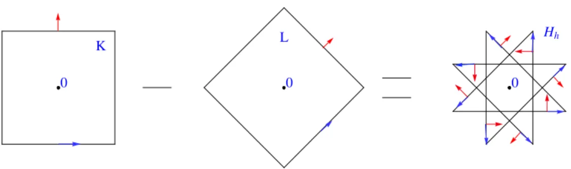
hedgehog with normal vector u. Let us give an example in R2. Let K and L be
the convex bodies of R2with support function h
K(x) = jhx; e1ij + jhx; e2ij and
hL(x) = jhx; e3ij + jhx; e4ij, where h:; :i is the standard inner product on R2,
(e1; e2) the canonical basis of R2 and e3; e4 2 R2 the unit vectors given by
e3= p12(e1+ e2) and e4= p12(e1 e2). These convex bodies are two squares
whose formal di¤erence K L can be realized geometrically as the hedgehog
with support function h = hK hL, which is a regular octagram constructed by
connecting every third consecutive vertex of a regular octogon (i.e., a regular star polygon with Schlä‡i symbol f8=3g): see Figure 3.
0 0 0
K L
Hh
Polytopal hedgehogs and hedgehogs with an analytical support function can also be introduced in index terms via Euler Calculus [13].
3
Complex hedgehogs in
C
n+1or
P
n+1(C)
3.1
Real and complex hedgehogs as dual hypersurfaces of
graphs
In order to introduce complex hedgehogs, it is convenient to recall that real hedgehogs with a smooth support function can be regarded as dual
hypersur-faces of smooth graphs. In what follows, any hedgehog Hh Rn+1 with
sup-port function h 2 C1(Sn; R) will be regarded as a hypersurface in the real
projective space Pn+1(R) by adding ‘a hyperplane at the in…nity’H
1to Rn+1:
Pn+1(R) = Rn+1[ H1. More precisely, we will identify Rn+1 with the a¢ ne
hyperplane of Pn+1(R) = Rn+2 f0g =R with equation Xn+2 = 1, where
[X1; : : : ; Xn+2] denote the homogeneous coordinates of the equivalent class of
(X1; : : : ; Xn+2) 2 Rn+2 f0g in Pn+1(R) : Then, the hedgehog hypersurface
xh: Sn! Hh Rn+1 Pn+1(R) can be regarded as the dual hypersurface of
h: Sn Rn+1 ! Pn+1(R)
u = (u1; : : : ; un+1) 7! [u1; : : : ; un+1; h (u)] :
Indeed, the support hyperplane with equation hx; ui = h (u) then corresponds
to the point h(u) by projective duality.
It is extremely natural to follow this idea to extend the notion of hedgehog
to the complex setting. We regard the complex Euclidean space Cn+1 as the
a¢ ne hyperplane of Pn+1(C) = Cn+2 f0g =C with equation Xn+2= 1, and
we de…ne, for any holomorphic function h : Cn ! C, the hedgehog with support
function h as the hypersurface of Cn+1that is the dual hypersurface of
h: Cn ! Pn+1(C)
z = (z1; : : : ; zn) 7! [1; z1; : : : ; zn; h (z)] ;
that is, as the envelope of the family of hyperplanes (Hh(z))z2Cn with equation
X1+ n X k=1 zkXk+1= h (z) : (1) In other words:
De…nition 1 Let h : Cn! C be a holomorphic function. The hypersurface H
h
of the complex Euclidean space Cn+1that is parametrized by
xh: Cn ! Cn+1 z = (z1; : : : ; zn) 7! h (z) n P k=1 zk @h @zk (z) ; @h @z1 (z) ; : : : ; @h @zn (z) is called the hedgehog with support function h.
Indeed, from (1) and the contact condition dw0+
Pn
j=1zjdwj = 0, where
(w0; w1; : : : ; wn; z1; : : : ; zn) 2 Cn+1 Cn = C2n+1, we deduce that for all z 2 Cn,
the point xh(z) = (x1(z) ; : : : ; xn(z)) is the unique solution of the system
8 > > > < > > > : x1+ n P k=1 zkxk+1= h (z) (1) 8k 2 f1; : : : ; ng ; xk+1= @h @zk (z) , (2)
where (2) is obtained from (1) by performing partial di¤erentiations with respect
to the complex variables zk, (1 k n). Thus, it appears that Hh is actually
parametrized by xh: Cn! Cn+1; z = (z1; : : : ; zn) 7! h (z) n X k=1 zk @h @zk (z) ; @h @z1 (z) ; : : : ; @h @zn (z) ! .
Example. The hedgehog C2 of which the support function h : C ! C is
given by h (z) = z3 is the a¢ ne algebraic curve H
h of C2 with equation 27x2+ 4y3= 0. It is parametrized by: 8 < : x = 2z3 y = 3z2:
As any complex hedgehog curve xh: C ! C2, it is such that:
8z 2 C, x0h(z) = h00(z) (z; 1) 2 C (z; 1) .
Naturally, we could have introduced complex hedgehogs of Cn+1in the
com-plex contact geometry setting, where they appear as fronts of Legendrian
im-mersions in C2n+1 (see the next subsection).
Remark. Of course, many other parametrizations would have been possible in order to introduce the notion of a complex hedgehog. New parametrizations can simply be obtained by performing chart changes. For instance, for any holomorphic function g : C ! C, the complex curve
yg : C ! C, xh: z 7 ! (g0(z) ; g (z) zg0(z))
is a hedgehog, namely the hedgehog with support function f (z) = zg (1=z): 8z 2 C , yg(z) = xf
1
z .
Therefore, this particular parametrization change only corresponds to the chart
3.2
Complex hedgehogs as fronts in
C
n+1of Legendrian
immersions in
C
2n+1Consider the complex Euclidean space C2n+1 endowed with the holomorphic
contact form ! := dw0+ n X j=1 zjdwj ;
where (w0; w1; : : : ; wn; z1; : : : ; zn) denote the canonical complex coordinates
func-tions on C2n+1. Recall that the projection
: Cn+1 Cn= C2n+1 ! Cn+1
(w; x) = (w0; w1; : : : ; wn; z1; : : : ; zn) 7 ! w = (w0; w1; : : : ; wn)
is called the front projection.
Then, for every holomorphic function h : Cn ! C, the map
ih: Cn ! Cn+1 Cn = C2n+1
z 7 ! (xh(z) ; z)
is a Legendrian immersion of Cn into C2n+1; ! (that is, i
h : Cn ! C2n+1
is a holomorphic immersion, and (Tzih) (Cn) Ker !ih(z) for all z 2 C
n) of
which Hh= xh(Cn) is the front ( ih) (Cn) in Cn+1.
Indeed, for all z = (z1; : : : ; zn) 2 Cn and i 2 f1; : : : ; ng, we have
@xh @zi (z) = 0 @ n X j=1 zj @2h @zi@zj (z) ; @ 2h @zi@z1 (z) ; : : : ; @ 2h @zi@zn (z) 1 A , and hence !ih(z) @xh @zi (z) ;@IdCn @zi (z) = n X j=1 zj @2h @zi@zj (z) + n X j=1 zj @2h @zi@zj (z) = 0.
3.3
Rational hedgehogs of the complex projective plane
P
2(C)
Here, we choose to work in the complex projective plane P2(C) equipped with
the usual Fubini-Study Kähler form ! (see e.g. [2]). For any (X1; X2; X3) 2
C3 f0g, [X
1; X2; X3] will denote the homogeneous coordinates of the
equiva-lent class of (X1; X2; X3) in P2(C) = C3=C .
Let h : C ! C be a holomorphic map such that the projective curve xh :
C ! P2(C), z 7! [xh(z) ; 1] = [zh (z) h0(z) ; h0(z) ; 1] satis…es
Then, the hedgehog curve xh: C ! P2(C) extends to a rational curve
xh: P1(C) ! P2(C)
z 7 ! xh(z) ,
which we call the rational hedgehog Hh:= xh P1(C) with support function
h : P1(C) ! P1(C) ; z 7 ! 8 < : h (z) if z 2 C lim z!1h (z) if z = 1.
Indeed Ahlfors lemma gives a description of rational curves as entire curves of bounded area ([3]):
“Let X be a compact complex manifold and f : C ! X an entire curve (i.e. a non constant holomorphic map) such that Area [f (C)] < +1. Then f
extends to a holomorphic map from P1(C) to X, a rational curve”.
3.4
Evolute of a plane complex hedgehog as locus of its
centers of curvature
In classical di¤erential geometry of curves, the evolute of a plane curve is the locus of all its centers of curvature or, equivalently, the envelope of its normal
lines. In particular, the evolute of a plane hedgehog Hh R2 with support
function h 2 C1 S1; R is the locus of all its centers of curvature c
h( ) :=
xh( ) Rh( ) u ( ), where Rh( ) := det Tu( )xh = (h + h00) ( ) is the
so-called curvature function of Hh, and u ( ) := (cos ; sin ), 2 S1= R=2 Z .
Equivalently, the evolute of Hh can be de…ned as the envelope of its ‘normal
lines’ Nh( ) := fxh( )g + Ru ( ), that is, the hedgehog H@h with support
function (@h) ( ) := h0 2 . Note that in the hedgehog case, the centers of
curvature ch( ) are well-de…ned for all 2 S1, even if x0h( ) = Rh( ) u ( ) is
the null vector, since the curvature function Rh( ) = (h + h00) ( ) is well-de…ned
for all 2 S1. Likewise, the normal line to Hh at xh( ) is well-de…ned, even
if x0
h( ) = 0, as the perpendicular Nh( ) to the support line hx; u ( )i = h ( )
through the point xh( ). For plane real hedgehogs, it is convenient to keep in
mind the following commutative diagram:
h: S1! P2(R) 7 ! [cos ; sin ; h ( )] P r o j e c t i v e d u a l i t y $ Xh: S1! R2 P2(R) 7 ! (xh( ) ; 1) d d # derivation @ # evolute 0 h: S1! P2(R) 7 ! [ sin ; cos ; h0( )] P r o j e c t i v e d u a l i t y $ (ch; 1) : S 1! R2 P2(R) 7 ! (ch( ) ; 1)
where ch( ) = x@h +2 , 2 S1 . The main purpose of this subsection is
to extend the notion of evolute to plane complex hedgehogs, together with its interpretation as locus of the centers of curvature. To this aim, we need to change our way of interpreting the transformation
d
d : S
1 R2 ! S1 R2
u ( ) = (cos ; sin ) 7 ! u0( ) = ( sin ; cos )
in the above diagram since we cannot consider the complex ‘normal lines’to a complex hedgehog without antiholomorphic data being involved. Our choice is
to identify S1 with the projective line P1(R) = R [ f1g and thus to consider
the transformation
P1(R) = R [ f1g ! P1(R) = R [ f1g
[cos ; sin ] = x 7! [ sin ; cos ] = 1
x :
In other words, we are going to consider the envelope of the family (L0
h(z))z2C
of complex lines of C2 given by L0
h(z) := fxh(z)g + C (z; 1). For all z 2 C,
L0
h(z) can be completed into a projective line \L0h(z) of P2(C) with equation
zX1 X2+ zh (z) 1 + z2 h0(z) X3= 0,
where [X1; X2; X3] denote the homogeneous coordinates of the equivalent class
of (X1; X2; X3) 2 C3 f0g in P2(C). Now, by projective duality, this family of
projective lines L\0
h(z)
z2C corresponds to the complex curve that is
parame-trized by
C ! P2(C)
z 7 ! z; 1; zh (z) 1 + z2 h0(z) .
Note that for z 6= 0, we have
z; 1; zh (z) 1 + z2 h0(z) = [1; w; (@h) (w)] ,
where w = z1 and (@h) (w) := h w1 + w +w1 h0 1
w .
Therefore, we have the following commutative diagram:
h: z 7! [1; z; h (z)] P r o j e c t i v e d u a l i t y $ Xh: z 7! [xh(z) ; 1] # @ # evolute @h: w = z1 7! [1; w; (@h) (w)] P r o j e c t i v e d u a l i t y $ (ch; 1) : z 7! x@h z1 ; 1
where ch(z) := x@h z1 = xh(z) 1 + z2 h00(z) (1; z). This expression of
curvature of a real hedgehog Hhat a point xh( ): ch( ) = xh( ) Rh( ) u ( ),
where Rh is the curvature function of Hh R2. We shall see below that
ch(z) := x@h z1 = xh(z) 1 + z2 h00(z) (1; z) can actually be interpreted
as the center of curvature of the complex hedgehog Hhat the point xh(z).
De…nition 2 Let h : C ! C be a holomorphic function. We shall say that the
complex hedgehog with support function (@h) (z) = h z1 + z +1z h0 1
z is
the evolute of the complex hedgehog Hh.
Fundamental examples. If h is the homomorphic function de…ned on the open disc D := fz 2 C jjzj < 1 g by h (z) = a1z+a0+
p
1 + z2, where (a
0; a1; ) 2 C3,
then the complex hedgehog Hh = xh(D) is reduced to the point f(a0; a1)g if
= 0, and it lies on the complex circle C ((a0; a1) ; ) C2 with equation
(X1 a0)2+(X2 a1)2= 2if 6= 0. In both cases, the evolute H@h= ch(D) is
reduced to the point f(a0; a1)g. Indeed, for all z 2 C, xh(z) = x1h(z) ; x2h(z) =
(h(z) zh0(z) ; h0(z)) is such that x1h(z) ; x2h(z) = a0+ p 1 + z2 zp z 1 + z2; a1+ z p 1 + z2 = (a0; a1)+ (1; z) p 1 + z2 and ch(z) = xh(z) 1 + z2 h00(z) (1; z) = xh(z) 1 + z2 (1 + z2)32 (1; z) p 1 + z2 = (a0; a1) :
More generally, let us replace h : D ! C, z 7! a1z + a0+
p
1 + z2 by any
holomorphic function of the form h : U ! C, z 7! a1z + a0+ q (z), where U is
a connected open subset of C f i; ig, and q (z) is the support function of the complex unit circle C ((0; 0) ; 1) in the neighbor of z, that is:
q (z) = 8 > > > > > > > > > > < > > > > > > > > > > : p 1 + z2 if jzj < 1 z s 1 + 1 z 2 if jzj > 1 z + " p 2 s 1 + z " z + " 2 if sign [Re (z)] = " 2 f 1; 1g .
We leave it to the reader to check that : (i) the complex hedgehog Hh= xh(U)
is reduced to the point f(a0; a1)g if = 0, and it lies on the complex circle
C ((a0; a1) ; ) with equation (X1 a0)2+(X2 a1)2= 2if 6= 0 ; (i) moreover,
in both cases, the evolute H@h= ch(U) is reduced to the point f(a0; a1)g.
De…nition 3 Let Hf and Hg be two complex hedgehogs in C2, and let z0 2 C
be such that xf(z0) = xg(z0). We shall say that Hf and Hg have a contact of
Given any complex hedgehog with holomorphic support function h : U ! C, where U is any connected open subset of C f i; ig, a straightforward
compu-tation shows that, for any z02 U, the hedgehog with support function
c : U ! C; z 7! ch(z) := c2h(z0) z + c1h(z0) + q (z0)3h00(z0) q (z) ;
(which is reduced to the point fch(z0)g if h00(z0) = 0, or which lies on the
complex circle with equation X1 c1h(z0) 2
+ X2 c2h(z0) 2
= q (z0)6h00(z0)2
if h00(z
0) 6= 0), has a contact of order 2 with Hh= xh(U) at xh(z0).
De…nition 4 Let h : U ! C be a holomorphic function where U is a connected
subset of C f i; ig. For any z02 U , we shall say that ch(z0) is the center
of curvature of Hh = xh(U) at xh(z0), and, if z0 2 U is a regular point of
xh : U ! C2 (that is, if h00(z0) 6= 0), we shall say that the complex circle with
equation X1 c1h(z0) 2 + X2 c2h(z0) 2 = q (z0)6h00(z0)2
is the osculating complex circle of Hh at xh(z0).
Naturally, we de…ne the complex curvature function of a hedgehog Hh =
xh(U) as follows.
De…nition 5 Let h : U ! C be a holomorphic function where U is a connected
subset of C f i; ig. We de…ne the curvature function of Hh= xh(U) to be
the function Rh: U ! C that is given by Rh(z) := q (z)3h00(z) for all z 2 U.
Thus, for any z 2 U, the center of curvature of Hh = xh(U) at xh(z) can
be expressed as follows: ch(z) = xh(z) Rh(z) u (z) , where u (z) := 1 + z 2 q (z)3u (z) 2 C ((0; 0) ; 1) .
Of course, this expression of ch(z) has to be compared to the one giving the
expression of the center of curvature of a real hedgehog Hh at a point xh( ):
ch( ) = xh( ) Rh( ) u ( ), where Rh is the curvature function of Hh R2.
Remark. With our de…nitions, the complex circle C ((a0; a1) ; ) C2with
equation (X1 a0)2+ (X2 a1)2 = 2, where (a0; a1; ) 2 C2 C , can be
locally regarded as a hedgehog with radius of curvature equal to (possibly
3.5
Real and imaginary parts of
H
hC
2regarded as
hedgehogs of
R
3We know that if f and g are taken to be the real and imaginary parts respectively of a holomorphic function h : C ! C, z = x + iy 7! h (z) = f (x; y) + ig (x; y), then f and g are harmonic functions satisfying the Cauchy-Riemann equations, that is, @f @x(x; y) = @g @y(x; y) and @f @y(x; y) = @g @x(x; y) ,
for all (x; y) 2 R2. The aim of this subsection is to show that, in this context, f
and g determine two hedgehogs HF and HGof R3that can be regarded globally
as the orthogonal projections of the complex hedgehog Hh of C2=R4 into e?2
and e?
1 respectively, where (e1; e2; e3; e4) is the canonical basis of R4and where
e?
i denotes the 3-dimensional subspace of R4that is orthogonal to ei(1 i 4).
These hedgehogs HF and HG of R3 will be modeled on the hemisphere S2+ of
S2 R C that is contained in R
+ C. To any z 2 C we associate the point
(z) := (1; z) = q
1 + jzj2 of S2+. The orthogonal projection map from C2 =R4
onto e?
i will be denoted by e?
i.
Proposition 6 Let h : C ! C be a holomorphic function the real and imaginary
parts of which are f and g respectively:
h (x + iy) = f (x; y) + ig (x; y) for all (x; y) 2 R2. We have then
e?
2 [xh(z)] = xF( (z)) and e?1 [xh(iz)] = xG( (z)) , where F and G are respectively de…ned by:
F ( (z)) =qRe (h (z)) 1 + jzj2
and G ( (z)) =Im (h (iz))q
1 + jzj2
We shall of course say that the hedgehogs HF and HG are the real and
imaginary hedgehog parts of Hh.
Proof. We …rst note that an easy computation making use of the
Cauchy-Riemann equations gives:
xh(z) = (x1(z) + iy1(z) ; x2(z) + iy2(z)) 2 C2
where 8 > > > > > > > > > < > > > > > > > > > : x1(z) = f (x; y) x@f@x(x; y) y@f@y(x; y) y1(z) = g (x; y) x@g@x(x; y) y @g @y(x; y) x2(z) = @f@x(x; y) = @g @y(x; y) y2(z) = @f@y(x; y) = @g@x(x; y) ,
for all z = x + iy, (x; y) 2 R2 .
Next, we consider the positively 1-homogeneous function F : R+ R2! R
given by F (X; Y; Z) := Xf Y X; Z X for all (X; Y; Z) 2 R+ R 2.
A straightforward computation then shows that the Euclidean gradient of F is given by rF (X; Y; Z) = f YX; Z X Y X @f @x Y X; Z X + Z X @f @y Y X; Z X ; @f @x Y X; Z X ; @f @y Y X; Z X
for all (X; Y; Z) 2 R+ R2. Thus,
xF( (z)) = rF ( (z))
= f (x; y) x@f@x(x; y) ( y)@f@y(x; y) ;@f@x(x; y) ; @f@y(x; y) = (x1(z) ; x2(z) ; y2(z)) = e?
2 [xh(z)] ,
for all z = x + iy, (x; y) 2 R2 . In the same manner, we can easily check that
xF( (z)) = (y1(iz) ; x2(iz) ; y2(iz)) = e?
1 [xh(iz)] for all z 2 C.
4
Towards a Brunn-Minkowski theory for
com-plex hedgehogs
As already mentioned above, the notion of a hedgehog curve or surface was born from the study of the Brunn-Minkowski theory. It is therefore permissible to think that the development of a ‘theory of mixed volumes for complex hedge-hogs’ (replacing Euclidean volumes by symplectic ones) might be a promising way of research. In this section, we will just mention …rst two observations.
4.1
Mixed symplectic area
Let C2 be the complex Euclidean space endowed with the standard Hermitian
inner product h:; :iC2. We are interested in the symplectic area of complex
hedge-hogs in this Kähler manifold C2; J; ! , where J is the complex structure and !
the 2-form ! (X; Y ) := Re (hJX; Y iC2). Any nontrivial complex hedgehog of C2
modeled on the unit disk D of C is a holomorphic curve (i.e. a nonconstant map
from the complex plane to C2). Now, it is well-known that the Riemannian area
of holomorphic curves is equal to their symplectic area, and hence that holomor-phic curves have positive area (the reader that is not familiar with holomorholomor-phic curves can …nd details in Subsection 1.1 of [17] ). An immediate consequence is the following result, which has to be compared to classical geometric inequalities for convex bodies (see [16, p. 369 and p. 382]).
Theorem 7 Let H (D) be the complex linear space of holomorphic functions
h : D ! C de…ned up to a similitude and consider Area [xh(D)] :=
Z
xh(D) !.
Then the map pA : H (D) ! R+, h 7!
p
Area [xh(D)] is a norm associated
with a scalar product (h; k) 7 ! A (h; k), which can be interpreted as a mixed
symplectic area. In particular, for any (h; k) 2 H (D)2, we have
p
A(h + k) pA(h) +pA(k)
and
A(h; k)2 A(h) A(k);
with equalities if, and only if, Hh and Hk are homothetic (here,“homothetic”
means that there exists ( ; ) 2 R2 f(0; 0)g such that h + k = 0).
4.2
A sharp estimation of the area using the energy
Note that we have the following sharp estimate of Area [xh(D)], which is better
than that well-known for an arbitrary smooth loop : S1! V in a symplectic
vector space (V; !) (namely, jA ( )j E ( ), see for instance [14, pp. 87-88]):
Theorem 8 Assume that h : D ! C is the sum of a power seriesPhnzn with
radius of convergence R > 1: h (z) = +1 X n=0 hnzn for all z 2 D. Then Area [xh(D)] 3 4E (xh) ,
where E (xh) is the energy of the loop xh : S1 = R=2 Z ! C2, 7! xh ei , that is: E (xh) := 1 2 Z 2 0 d d xh e i 2 d .
Furthermore, the equality holds if, and only if, the function h is of the form h (z) = amzm+ a1z + a0, where m 2 N and (a0; a1; am) 2 C3.
Proof. Consider the Fourier expansion of H ( ) := h ei on S1= R=2 Z:
H ( ) :=
+1
X
n=0
hhein .
An easy computation immediately gives:
8 2 S1, xh( ) :=
+1
X
n=0
ein ((1 n) hn; (n + 1) hn+1) .
Using the formula known for the action A ( ) := (1=2)R02 ! ( ( ) ; 0( )) d of
an arbitrary smooth loop : S1 ! C2 (see e.g. at the top of the page 88 in
[14]), we then deduce that:
Area [xh(D)] = A (xh) =
+1
X
n=0
n (n 1)2jhnj2+ (n + 1)2jhn+1j2 .
Separating into two sums and re-indexing in the …rst one, we then obtain: Area [xh(D)] = +1 X n=1 n (n + 1) (2n + 1) jhn+1j2= 6 +1 X n=1 n X k=1 k2 ! jhn+1j2.
On the other hand, we have: 8 2 S1,
d d xh e i = e i (H0( ) + iH00( )) ei ; 1 and hence d d xh e i 2 = 2 jH0+ iH00j ( )2= 2 jH00 iH0j ( )2= 2 h00 ei 2: Therefore Parseval’s identity yields:
E (xh) := 1 2 Z 2 0 d d xh e i 2 d = Z 2 0 h00 ei 2d = 8 +1 X n=1 n X k=1 k !2 jhn+1j2, since h00(z) = +1 X n=1 n (n + 1) hn+1zn 1= 2 +1 X n=1 n X k=1 k ! hn+1zn 1:
5
Real hedgehogs in
C
n=
R
2nand their evolutes
In the Euclidean plane, the evolute of a hedgehog is the locus of all its centers of curvature or, equivalently, the envelope of its normal lines. In order to …nd an analogue in any even higher dimension, we make use of the following trick. First,
we …x a linear complex structure J on R2n (that is, an endomorphism J of R2n
such that J2= IdR2n). Given any hedgehog with smooth support function h in
R2n, we then de…ne the normal hyperplane to Hh at a point xh(u), say Nh(u),
as the a¢ ne hyperplane fxh(u)g+J u? , where u?is the (2n 1)-dimensional
subspace of R2n that is orthogonal to u. Finally, we de…ne the evolute of H
h in
R2n; J as the envelope of the family of normal hyperplanes (N
h(u))u2S2n 1 in
R2n. Let us begin by considering carefully the four dimensional case.
5.1
Evolutes of hedgehogs hypersurfaces in
R
4In what follows, we identify R4with the quaternion algebra H and thus the unit
sphere S3to the set S1
Hof unit quaternions. To any pure unit quaternion v, we
associate the linear complex structure Jv: R4! R4, x 7 ! vx. We denote by !v
the associated Kähler form (i.e. the alternating 2-form !v(X; Y ) = hJvX; Y i,
where h:; :i is the standard Euclidean metric on R4 . Recall that we can retrieve
h:; :i from !v: hX; Y i = !v(X; JvY ). Particularizing our de…nition of evolute
hedgehogs to the four dimensional case, we get the following de…nition.
De…nition 9 Let h 2 C1 S3; R . We de…ne the evolute of Hh in the Kähler
vector space R4; J
v; !v to be the envelope of the family of normal hyperplanes
(Nv
h(u))u2S3 with equation
hx xh(u) ; Jv(u)i = 0.
Proposition 10 Let h 2 C1 S3; R . The evolute of H
h in R4; Jv; !v is the
hedgehog H@vh with support function
@vh : S3! R, u 7 ! hrh ( Jv(u)) ; ui ,
where h:; :i is the standard Euclidean metric on R4, and rh the gradient of h.
Proof. Since Jv: R4! R4is an isometry such that Jv2= IdR4, the evolute of Hh in R4; Jv; !v can be regarded as the envelope of the family of hyperplanes
(Nhv( Jv(u)))u2S3 with equation
hx xh( Jv(u)) ; ui = 0,
that is, as the hedgehog H@vh of R
4with support function
Remark 11 By abuse of language, the hedgehog with support function @vh will
also be called ‘the evolute of Hh with respect to (the pure unit) quaternion v’.
Parametrization of the evolute of H@vh and interpretation
It follows immediately from de…nitions that x@vh: S
3! R4 associates with
each u 2 S3 the unique solution of the system
hx; Jv(u)i = hxh(u) ; Jv(u)i
8X 2 TuS3, hx; Jv(X)i = hTuxh(X) ; Jv(u)i + hxh(u) ; Jv(X)i ,
which is equivalent to
hx xh(u) ; Jv(u)i = 0
8X 2 TuS3, hx xh(u) ; Jv(X)i = hJv(Tuxh(Jv(u))) ; Jv(X)i ,
because hTuxh(X) ; Jv(u)i = hTuxh(Jv(u)) ; Xi = hJv(Tuxh(Jv(u))) ; Jv(X)i
since Tuxh is a symmetric endomorphism of TuS3 and Jv an isometry of R4.
Therefore:
8u 2 S3, x@vh(u) = xh(u) + Jv(Tuxh(Jv(u))) = xh(u) + vTuxh(Jv(u)) . In other words, we have the following.
Proposition 12 Let h 2 C1 S3; R and let v be a pure unit quaternion. For
all u 2 S3,
x@vh(u) = xh(u) Rh(u; v) u,
where Rh(u; v):= vTuxh(Jv(u)) u; here u of course refers to the quaternion
conjugate of u.
Comparison to the planar case and interpretation
This expression of x@vh(u) has to be compared to the one of the center of
curvature of a plane hedgehog Hh at a point xh( ):
ch( ) := xh( ) Rh( ) u ( ) ,
where Rh:= h + h00 is the curvature function of Hh. Identifying R2 to C, and
thus Tu S1 with R(iei ), this last formula can be rewritten as
ch ei := xh ei Rh ei ei ,
where Rh ei := iTu xh iei e i .
Rh(:; v) : u := (cos ) u + (sin ) vu 7 ! Rh(u ; v) can be interpreted as a
quaternionic curvature function of xh S1u;v , where S1u;v denotes the unit
circle of the vector plane C (u; v) := Ru + RJv(u) oriented by (u; Jv(u)).
The reason why Rh ei is a real number for h 2 C1 S1; R , when Rh(u; v) is
a quaternion for h 2 C1 S3; R , comes from the fact the product of two purely
imaginary complex numbers is a real number, when the product of two pure quaternions is a quaternion.
Complement to the planar case
We introduced “the” evolute H@h of a plane hedgehog Hh as the envelope
of its normal lines. But in fact they are two of them if we take into account the choice of coorientation of the normal line. Of course, we could have introduce
evolutes of hedgehog curves in R2 in the same way as we have just done for
evolutes of hedgehogs hypersurfaces in R4. Identifying R2 with the complex
plane C, we can associate to any v 2 f i; ig the linear complex structure Jv :
C ! C, x 7 ! vx and the associated Kähler form !v(X; Y ) = hJvX; Y i, where
h:; :i is the standard Euclidean metric on R2, and then, de…ne the evolute of
the plane hedgehog with support function h 2 C1 S1; R in R2; J
v to be the
envelope H@vhof the family of normal lines (N
v
h(u))u2S1 with equation hx xh(u) ; Jv(u)i = 0.
If we do so, we can immediately check that H@vh has support function
@vh : S1! R, u 7 ! hrh ( Jv(u)) ; ui .
In other words, (@ih) ( ) = h0( =2) and (@ ih) ( ) = h0( + =2) for all
2 S1= R=2 Z.
Note that, in the 2 or 4-dimensional case, the evolutes H@vh and H@ vhare
one and the same hypersurface of R2n (n = 1; 2) but corresponding to opposite
coorientations of the normal hyperplanes of Hh:
(@ vh) (u) = hrh ( J v(u)) ; ui = hrh ( Jv( u)) ; ui = (@vh) ( u) .
Geometrical interpretation of the Hodge Laplacian
Taking the Hodge Laplacian of h 2 C1 S1; R is tantamount to taking the
evolute in R2; J
i of the evolute of Hhin R2; J i , or conversely, the evolute
in R2; J
i of the evolute of Hh in R2; Ji . Indeed, for any h 2 C1 S1; R ,
we have (@i @ i) (h) = (@ i @i) (h) = h00 = h, where is the Hodge
Laplacian on S1.
This result can be extended as follows to dimension 4. Let h 2 C1 S3; R
and u 2 S3. If v is a pure unit quaternion such that J
v(u) is an eigenvector of
@ v(@vh) (u) = @v(@vh) ( u) = @2vh ( u) = @2vh Jv2(u)
= r2h u(Jv(u) ; Jv(u)) = .
Therefore, if v1; v2; v3are pure unit quaternions such that Jv1(u) ; Jv2(u) ; Jv3(u)
are eigenvectors of the Riemannian Hessian r2h u, corresponding to
eigenval-ues 1, 2, 3, that form an orthonormal basis of TuS3, then:
h (u) = X3
i=1 i(u) =
X3
i=1(@ vi @vi) (h) (u) .
Decomposition of hedgehogs into sums of remarkable pedal hyper-surfaces
Let (v; w) be any couple of pure unit quaternions that are orthogonal when
they are regarded as vectors of R4. The quadruple (1; v; w; vw) is then a direct
orthonormal basis of H = R4. For any hedgehog of R4 with support function
h 2 C1 S3; R and, for any u 2 S3, we have the following decompositions
xh(u) = h (u) u + rh (u)
= h (u) u + (hrh (u) ; vui vu + hrh (u) ; wui wu + hrh (u) ; vwui vwu) = h (u) u + @vh (vu) vu + @wh (wu) wu + @vwh (vwu) vwu
= (h (u) + @vh (vu) v + @wh (wu) w + @vwh (vwu) vw) u
In particular, the hedgehog xh: S3! H = R4is the sum of parametrizations
of 4 remarquakable pedal surfaces: its own pedal surface and the pedal surfaces of its evolutes with respect to v, w,vw (it being understood that, for all u 2 S3,
and, any pure unit quaternion q, we take the foot of the perpendicular from the
origin to the support hyperplane with unit normal vector Jq(u) := qu).
Evolutes and orthogonal projections
For every (u; v) 2 S3 S2, let S1u;v be the oriented geodesic of S3 through
u in the direction of Jv(u). This oriented circle of S3 can be regarded as the
unit circle of the vector plane C (u; v) := Ru + RJv(u) oriented by (u; Jv(u)).
Restriction of support functions to S1
u;v commutes with taking the evolutes in
R4; J v; !v :
Proposition 13 Let h 2 C1 S3; R . For all v 2 S2=S1
H\ Im (H),
(@vh)jS1
u;v = @v hjS 1 u;v :
Proof. De…ne u := (cos ) u + (sin ) Jv(u) for all 2 S1. We have then
(@vh) (Jv(u )) = hrh (u ) ; Jv(u )i =
d
Higher order evolutes
Of course, we can de…ne inductively higher order evolutes. Let @0
vh = h and,
for any positive integer n, de…ne the nth evolute of Hh in R4; Jv; !v to be the
hedgehog with support function @n
vh := @v @vn 1h .
Proposition 14 Let C1 S3; R . For all n 2 N , v 2 S2, and u 2 S3,
(@vnh) (Jvn(u)) = d
n
d n [h (u )]j =0,
where u := (cos ) u + (sin ) Jv(u).
Proof. By induction, we deduce from the previous proposition that
8n 2 N , (@vnh)jS1 u;v = @
n v hjS1
u;v , and the result follows immediately.
5.2
Symplectic and mixed symplectic area
Any pure unit quaternion v determines a linear complex structure Jv : R4! R4,
to which it corresponds a Hopf ‡ow induced on S3 = S1
H by the vector …eld
Xv(u) := Jv(u). We denote by S2the set S3\ Im (H) of pure unit quaternions.
For every (u; v) 2 S3 S2, let S1
u;v be the oriented geodesic of S3 through u
in the direction of Jv(u). This oriented Hopf circle of S3 R4; Jv can be
regarded as the unit circle of the vector plane C (u; v) := Ru + RJv(u) oriented
by (u; Jv(u)). Conversely, any oriented vector plane in R4 determines an
oriented unit circle S1= S3\ and a pure unit quaternion v that is such that:
8u 2 S1, T
uS1is oriented by the unit vector Jv (u).
Now, consider the integral
s (h) := Z
xh(S1)
v ,
where v is the 1-form given by v x(dx) =12!v (x; dx), which is such that
d v = !v . This integral does not depend on the orientation of the plane
(if we change the orientation of , the orientation of the curve xh : S1 ! R4
changes as well and the 1-form v is changed into its opposite). Therefore,
s (h) can be de…ned for any unoriented vector plane in R4. It will be called
the symplectic area of xh S1 relative to .
Expression of the symplectic area of xh S1u;v
Let su;v(h) be this symplectic area:
su;v(h) :=
Z
xh(S1u;v)
where av is the 1-form given by ( v)x(dx) := 12!v(x; dx) = 1
2hx; ( Jv) (dx)i.
Proposition 15 For all h 2 C1 S3; R and (u; v) 2 S3
S2, su;v(h) = 1 2 Z 2 0 hx h(u ) ; Rh(u ; v) u i d ,
where u := (cos ) u + (sin ) Jv(u) and Rh(u ; v) := v (Tu xh) (Jv(u )) u .
Proof. By de…nition su;v(h) := Z xh(S1u;v) v= 1 2 Z 2 0 xh(u ) ; ( Jv) d d [xh(u )] d . Now d d [xh(u )] = (Tu xh) (Jv(u )) and hence ( Jv) d d [xh(u )] = v (Tu xh) (Jv(u )) = Rh(u ; v) u .
Proposition 16 For all h 2 C1 S3; R and (u; v) 2 S3 S2,
su;v(h) = au;v(h) + s?u;v(rh)
where au;v(h) is the algebraic area of the hedgehog of C (u; v) = Ru + RJv(u)
whose support function is the restriction of h to S1
u;v, and where s?u;v(rh) is the
symplectic area of rh S1
u;v in the Kähler vector space R4; Jv; !v , that is,
s?u;v(rh) := Z rh(S1 u;v) v = 1 2 Z rh(S1 u;v) !v(x; dx) .
Proof.It is just the fact that the symplectic area of a closed curve in the Kähler vector space R4; J
v; !v is the sum of the algebraic areas of its projections onto
the planes C (u; v) and C (u; v)?. In the present case, we can retrieve the result as follows. Let 2 S1. We have x h(u ) = h (u ) u + rh (u ), and Rh(u ; v) u = ( Jv)(Tu xh(Jv(u ))) = ( Jv) h (u ) Jv(u ) + rJv(u )rh (u ) = h (u ) u + ( Jv) rJv(u )rh (u ) ,
where r is the Levi-Civita connection on S3. In addition, u ; ( Jv) rJv(u )rh (u ) = Jv(u ) ; rJv(u )rh (u ) = dd [hJv(u ) ; rh (u )i] = d 2 d 2[h (u )] , and rh (u ) ; ( Jv) rJv(u )rh (u ) = !v rh (u ) ; d d [rh (u )] since d d [rh (u )] = rJv(u )rh (u ) hrh (u ) ; Jv(u )i u . Hence xh(u ) ; ( Jv) d d [xh(u )] = h(u ) h(u ) + d2 d 2[h(u )] +!v rh(u ); d d [rh(u )]
The result is then an immediate consequence of the previous proposition. Mixed symplectic area
Proposition 17 (Symmetry) For all (f; g) 2 C1 S3; R 2, and (u; v) 2 S3 S2,
Z 2 0 hx f(u ) ; Rg(u ; v) u i d = Z 2 0 hx g(u ) ; Rf(u ; v) u i d .
Proof. For all 2 S1,
d
d [!v(xf(u ) ; xg(u ))] = !v(Tu xf(Jv(u )) ; xg(u ))+!v(xf(u ) ; Tu xg(Jv(u ))) . By integration, we deduce that
Z 2 0 !v(xf(u ) ; Tu xg(Jv(u ))) d = Z 2 0 !v(xg(u ) ; Tu xf(Jv(u ))) d ,
which is the desired equality since
!v(xh(u ) ; Tu xh(Jv(u ))) = hJvxh(u ) ; Tu xh(Jv(u ))i
= hxh(u ) ; Jv[Tu xh(Jv(u ))]i
= hxh(u ) ; Rh(u ; v) u i
for h 2 ff; gg.
De…nition 18 Let (f; g) 2 C1 S3; R 2 and (u; v) 2 S3 S2. We call
su;v(f; g) :=
1
2(su;v(f + g) su;v(f ) su;v(g)) = 1 2
Z 2
0 hx
f(u ) ; Rg(u ; v) u i d
A straightforward computation shows that
su;v(f; g) = au;v(f; g) + s?u;v(rf; rg) ,
where au;v(f; g) is the mixed symplectic area of the hedgehogs of C (u; v) with
support functions fjS1
u;v and gjS1u;v, and where s
?
u;v(rf; rg) is the mixed
sym-plectic area of rf S1
u;v and rg S1u;v in R4; Jv; !v , that is,
s?
u;v(rf; rg) := 12 s?u;v(r (f + g)) s?u;v(rf) s?u;v(rg)
=1 2 Z 2 0 !v rf(u );dd [rg(u )] d =1 2 Z 2 0 !v rg(u );dd [rf(u )] d . Symplectic area of Hh
De…nition 19 Let h 2 C1 S3; R . We de…ne the symplectic area of H
h to be s (h) := v4 v2 Z G4;2 s (h) d!4;2( ) ,
where vn is the volume of the unit ball in Rn+1, G4;2 the Grassman manifold of
2-dimensional subspaces of R4 and !
4;2 the normalized Haar measure on G4;2:
!4;2(G4;2) = 1.
Recall that the mixed volume V : K4 4 ! R extends to a symmetric
4 linear form on the vector space H4of hedgehogs of R4. Besides, the algebraic
area of order 2 of a hedgehog Hhof R4, denoted by V2(h), is de…ned to be the
mixed volume V (h; h; 1; 1).
Proposition 20 For any h 2 C1 S3; R , the symplectic area of H
h is equal
to its algebraic area of order 2, that is, s (h) := V2(h).
Proof. From Kubota’s formula
V2(K) = v4 v2 Z G4;2 V (p (K)) d!4;2( ) ,
for all convex body K in R4, where p (K) is the orthogonal projection of K
on 2 G4;2, V (p (K)) its area and V2(K) the mixed volume V (K; K; B; B),
B denoting the unit ball in R4 (see [16, Section 5.3]). This formula can be
extended to hedgehogs by multilinearity, so that: v2(h) = v4 v2 Z G4;2 a hjS1 d!4;2( ) ,
for all h 2 C1 S3; R . Note that the algebraic area of HhjS1 does not depend
on a choice of orientation for . Now, we have proved above that su;v(h) = a hjS1
u;v + s
? u;v(rh)
for all (u; v) 2 S3 S2. So, it su¢ ces to prove that for all u 2 S3, Z
S2
!v rh (u) ; rJv(u)rh (u) d (v) = 0,
where is the spherical Lebesgue measure.
Now, let (v1; v2; v3) 2 S2= SH1\Im (H) be such that (Jv1(u) ; Jv2(u) ; Jv3(u))
is an orthonormal basis of TuS3 formed by eigenvectors of the Riemannian
Hessian r2h u, corresponding to eigenvalues ( 1; 2; 3). A straightforward
calculation then gives, for any v =P3i=1xivi2 S2,
( Jv) rJv(u)rh (u) = ( Jv) 0 @ 3 X j=1 xj jJvj(u) 1 A = 3 X i;j=1 xixj i jvivju = X 1 i<j 3 xixj( i j) vivju and hence Z S2
!v rh (u) ; rJv(u)rh (u) d (v) =
Z S2 ( Jv) rJv(u)rh (u) d (v) = X 1 i<j 3 0 B B @ Z S2 xixjd | {z } =0 1 C C A ( i j) vivju. = 0; which achieves the proof.
5.3
Quaternionic curvature function
Let K be a convex body with class C1
+ in (n + 1)-Euclidean vector space Rn+1.
One says that K has the (C1-smooth) curvature function RK : Sn ! R if its
surface area measure Sn(K; :) as RK a density with respect to spherical area
measure or, equivalently, if
V (L; K; : : : ; K) =n+11 Z
Sn
hL(u) RK(u) d (u)
= 1
n+1
Z
SnhxhL
for all convex body L with support function hL: Sn! R (see e.g. [16, p. 545]).
The notion of curvature function naturally extends to C2-hedgehogs of Rn+1
[10]. The aim of this subsection is to use the notion of the mixed symplectic area of xg S1u;v and xh S1u;v to introduce the notion of the (quaternionic) curvature
function of xh S1u;v . As we already mentioned, the reason why Rh ei is a
real number for h 2 C1 S1; R , when R
h(u; v) is a quaternion for C1 S3; R ,
comes from the fact the product of two purely imaginary complex numbers is a real number, when the product of two pure quaternions is a quaternion.
Proposition 21 Let h 2 C1 S3; R , and (u; v) 2 S3 S2. There exists one
and only one C1-smooth quaternionic function R (:; v) : S1
u;v! H that is of the
form
u := (cos ) u + (sin ) vu 7 ! R (u ; v) = vTu (v) ;
where Tu (v) denotes a pure quaternion, and such that:
8g 2 C1 S3; R , su;v(g; h) := 1 2 Z 2 0 hx g(u ) ; R (u ; v) u i d ,
where u := (cos ) u + (sin ) vu. Namely, the quaternionic function given by: Rh(u ; v) := v (Tu xh) (vu ) u for all 2 S1.
Proof. For all 2 S1, T
u S3= Im (H) u and hence (Tu xh) (vu ) u 2 Im (H).
Thus, Rh(:; v) : u 7 ! Rh(u ; v) = v (Tu xh) (vu ) u is of the required form
since 8g 2 C1 S3; R , su;v(g; h) := 1 2 Z 2 0 hx g(u ) ; Rh(u ; v) u i d .
Conversely, let R (:; v) be any function satisfying the required conditions.
Note that the map u 7! R (u ; v) u has then the form u 7! (u ) u + ?(u ),
where 2 C1 S1
u;v; R and ?2 C1 S1u;v; C (u; v)? . Indeed, we have
hR (u ; v) u ; Jv(u )i = hJv( Tu (v) u ) ; Jv(u )i = h Tu (v) u ; u i = 0
for all 2 S1, since T
u (v) u 2 Im (H) u = Tu S3. Besides, in the case where
R (:; v) = Rh(:; v), we have R (u ; v) u = Rh(u ; vu ) u v ?u;v[rvu rh (u )],
where Rh(u ; vu ) is the radius of curvature of xhjS1
u;v : S
1
u;v ! C (u; v) at
xhjS1
u;v(u ) (or, equivalently, the tangential radius of curvature of Hh at xh(u )
in the direction vu , which is given by: Rh(u ; vu ) := hTu xh(vu ) ; vu i =
h (u ) + r2h u (vu ; vu ); see e.g. [10]), and ?
u;v the orthogonal projection
onto the subspace of R4 that is orthogonal to C (u; v). Indeed,
Rh(u ; v) u = v (Tu xh) (vu )
= v (h (u ) vu + rvu rh (u ))
= v h (u ) + r2h u (vu ; vu ) vu + ?
We already know that S1u;v! R; u 7! Rh(u ; vu ) is the unique C1-smooth
function R : S1u;v! R that satis…es:
8g 2 C1 S1u;v; R , au;v(g; h) := 1 2 Z 2 0 g (u ) R (u ) d . Now, any g 2 C1 S1
u;v; R can be extended into a function gS 2 C1 S3; R
that is such that ?u;v
h
(rgS)jS1 u;v
i
= 0: it su¢ ces, for instance, to de…ne gS by
8q 2 S3, gS(q) := 8 > < > : 0 if kpk = 0 z (kpk) g kpkp if kpk 6= 0,
where p is the orthogonal projection of q onto C (u; v) and,
z (t) := Z t 0 ' ( ) ' (1 ) d Z 1 0 ' ( ) ' (1 ) d ,
where ' is the function de…ned on R by ' (t) := 8 < : 0 if 0 e t21 if > 0. .
(F : R ! R is C1-smooth, and such that F (0) = 0, F (1) = 1, and: 8n 2 N ,
F(n)(0) = F(n)(1) = 0). For any g 2 C1 S1
u;v; R , such an extension gS is
such that su;v(gS; h) = au;v(g; h) = 1 2 Z 2 0 g (u ) (u ) d , since s?
u;v(rgS; rh) = 0. Therefore (u ) = Rh(u ; vu ) for all 2 S1.
Now, it remains to prove that ?(u ) = v ?
u;v[rvu rh (u )] for all 2 S1.
Since (u ) = Rh(u ; vu ) for all 2 S1, the integral condition can rewritten
as follows: 8g 2 C1 S3; R , s?u;v(g; h) := 1 2 Z 2 0 D rg (u )?; ?(u ) E d , where rg (u )? := ?u;v[rg (u )], that is,
8g 2 C1 S3; R , Z 2 0 D rg (u )?; ?(u ) + v ?u;v[rvu rh (u )] E d .
Note that rg (u )? has the form
where w is a pure unit quaternion that is h:; :i orthogonal to v, so that (v; w; vw)
is an orthonormal basis of Im (H). Moreover, ?(u ) + v ?u;v[rvu rh (u )] has
the form ( (u ) + (u ) v) wu , where and are real, since it belongs to
Rwu + Rvwu = C (u; v)?. Thus, the integral condition is that the function
S1u;v ! C (u; v)?, u 7 ! ?(u ) + v ?u;v[rvu rh (u )] is L2-orthogonal to all
the functions S1
u;v! C (u; v)?, u 7 ! rg (u )? where g 2 C1 S3; R . Now,
for any two real C1-functions a,b on S1
u;v, let us de…ne g : S3! H by:
g (q ( ; ; )) := [a (u ) hq ( ; ; ) ; wu i + b (u ) hq ( ; ; ) ; vwu i] F (cos ) , where
q ( ; ; ) = (cos ) u + (sin ) ((cos ) wu + (sin ) vwu ) 2 S3
= (cos ) (cos ) u + (cos ) (sin ) vu+
(cos ( ) (sin )) wu + (sin ( )) (sin ) vwu.
We then obtain @ @ [g (q ( ; ; ))]j =0 = D rg (q ( ; 0; )) ;@q@ ( ; 0; ) E = hrg (u ) ; (cos ) wu + (sin ) vwu i
= a (u ) cos + b (u ) sin ,
and thus, for = 0 and = =2, we have respectively a (u ) = hrg (u ) ; wu i
and b (u ) = hrg (u ) ; vwu i : In other words, all the functions of the form S1
u;v ! C (u; v)?, u 7 ! (a (u ) + b (u ) v) wu can be written in the form
S1
u;v! C (u; v)?, u 7 ! rg (u )? where g 2 C1 S3; R .
Therefore, ?(u ) = v ?
u;v[rvu rh (u )] for all 2 S1.
De…nition 22 For every h 2 C1 S3; R , we say that R
h(:; v) : S1u;v ! H,
u 7 ! v (Tu xh) (vu ) u is the quaternionic curvature function of xh S1u;v .
5.4
Convolution of hedgehogs
Di¤erences of (arbitrary) convex bodies of R2do not only constitute a real vector
space H2; +; : but also a commutative and associative R-algebra. Indeed, as
noticed by H. Görtler in [5] and [6], we can de…ne the convolution product of
two plane hedgehogs Hf and Hg in R2 as the plane hedgehog whose support
function is given by (f g) ( ) = 1 2 Z 2 0 f ( ) g ( ) d ,
for all 2 S1; and we can check at once that H2; +; :; is then a commutative
and associative algebra. H. Görtler also noticed that the convolution product of two plane convex bodies is still a plane convex body. The interest of convolution of hedgehogs is that properties of one factor are often transmitted to the product.
Of course, we think immediately of regularity properties but we also mentioned the following properties in [12]: to be centered (centrally symmetric with center at the origin), to be projective (i.e., to have an antisymmetric support function), to be of constant width.
A natural way of de…ning a (non-abelian) convolution product on the vector
space Hn+1of arbitrary hedgehogs of Rn+1is to proceed as follows: 1. First, we
identify Snwith the homogeneous space G=H, where G is the group SO (n + 1)
of rotations of Rn+1 and H the stabilizer subgroup of G with respect to the
north pole of Sn, say (that is, the subgroup H of G formed by the rotations
r 2 G that leave …xed); any support function h : Sn! R can thus be regarded
as a function h : G ! R such that h (rs) = h (r) for all (r; s) 2 G H; 2. Next,
given any two arbitrary hedgehogs Hf and Hg of Rn+1, we can de…ne their
convolution product Hf Hg as the hedgehog Hf g with support function
(f g) (r) =
Z
G
f rt 1 g (t) dmG(t) for all r 2 G,
where mGis the normalized Haar measure on G. This construction of Hf Hgis
essentially due to E. Grindberg and G. Zhang [7]. As expected, this convolution product behaves well with respect to expansions in series of spherical harmonics, and properties of one factor are often transmitted to the product (for instance, to be centred, projective, convex, of constant width, or a zonoid).
But of course, in the case of hedgehogs of R4 it is simpler to make use of
quaternions and thus to de…ne the convolution product Hf Hg of Hf and Hg
in R4 to be the hedgehog Hf g with support function
(f g) (u) =
Z
S3
f (vu) g (v) d (v) for all u 2 S1H=S3,
where is the spherical Lebesgue measure on S3.
5.5
Evolutes of hedgehogs hypersurfaces in
H
n=
R
4nWe identify R4n with the hyperkähler vector space (Hn; h:; :i ; I; J; K), where
h:; :i is the standard Euclidean metric on R4n = Hn, (n 1), and, the triple
of complex structures (I; J; K) on Hn is given by left multiplication by i; j; k
respectively. On this hyperkähler vector space, we have a whole S2 family of
linear Kähler structures given by:
Ia:= a1I + a2J + a3K and !a(X; Y ) = hIa(X) ; Y i ,
for all a = (a1; a2; a3) 2 S2 R3and, (X; Y ) 2 (TqHn)2. Most of the results we
saw for evolutes of hedgehogs in R4=H can be extended to (Hn; h:; :i ; I; J; K)
with a few adaptations. In particular, for all h 2 C1 S4n 1; R , the evolute
of the hedgehog Hh in the Kähler vector space R4; Ia; !a is de…ned to be the
envelope of the family of normal hyperplanes (Na
h(u))u2S4n 1 with equation hx xh(u) ; Ia(u)i = 0.
Proposition 23 Let h 2 C1 S4n 1; R . The evolute of Hh in (Hn; Ia; !a) is
the hedgehog H@ah with support function
@ah : S4n 1! R, u 7 ! hrh ( Ia(u)) ; ui ,
where h:; :i is the standard Euclidean metric on R4n =Hn, and rh the gradient
of h. Thus, @ah is such that: 8u 2 S
0n 1 ,
(@ah) (Ia(u)) = hrh (u) ; Ia(u)i = (dh)u(Ia(u)) .
The proof (very similar to that of the proposition concerning evolutes of hedgehogs in (H; Jv; !v), v 2 S2= S3\ Im (H) is left to the reader.
References
[1] A. D. Aleksandrov, Zur Theorie der gemischten Volumina von konvexen
Körpern, I:Verallgemeinerung einiger Begri¤ e der Theorie der konvexen Körper (in Russian). Mat. Sbornik N. S. 2 (1937), 947–972.
[2] A. Cannas da Silva, Lectures on Symplectic Geometry. Lectures Notes in
Mathematics, 1764, Springer-Verlag, Berlin, 2001 and 2008.
[3] J. Duval, Around Brody, 2017: https://arxiv.org/pdf/1703.01850v1.pdf
[4] H. Geppert, Über den Brunn-Minkowskischen Satz. Math. Z. 42 (1937),
238-254.
[5] H. Görtler, Erzeugung stützbarer Bereiche I. Deutsche Math. 2 (1937),
454-456.
[6] H. Görtler, Erzeugung stützbarer Bereiche II. Deutsche Math. 3 (1937),
189-200.
[7] E. Grindberg and G. Zhang, Convolutions, transforms, and convex
bod-ies. Proc. London Math. Soc. 78 (1999), 73-115.
[8] R. Langevin, G. Levitt and H. Rosenberg, Hérissons et
multihéris-sons (enveloppes paramétrées par leur application de Gauss). In: Singu-larities, Banach Center Publ. 20, Warsaw, PWN, 1988, 245-253.
[9] Y. Martinez-Maure, De nouvelles inégalités géométriques pour les
héris-sons. Arch. Math. 72 (1999), 444-45.
[10] Y. Martinez-Maure, Hedgehogs and zonoids. Adv. Math. 158 (2001), 1-17. [11] Y. Martinez-Maure, Contre-exemple à une caractérisation conjecturée de
la sphère. C. R. Acad. Sci. Paris, Sér. I, 332 (2001), 41-44.
[12] Y. Martinez-Maure, Geometric study of Minkowski di¤ erences of plane convex bodies. Canad. J. Math. 58 (2006), 600-624.
[13] Y. Martinez-Maure, Hedgehog theory via Euler Calculus. Beitraege zur Algebra und Geometrie 56 (2015), 397-421.
[14] D. McDuff and D. Salomon, J -holomorphic curves and symplectic topol-ogy. Colloquium Publications, American Mathematical Society 52, 2012. [15] G. Panina, New counterexamples to A. D. Alexandrov’s hypothesis. Adv.
Geom. 5 (2005), 301-317.
[16] R. Schneider, Convex Bodies: The Brunn-Minkowski Theory, 2nd ex-panded ed. Cambridge Univ. Press, 2014.
[17] C. Wendl, Lectures on Holomorphic Curves in Symplectic and Contact Geometry, 2014: https://arxiv.org/pdf/1011.1690.pdf
Y. Martinez-Maure
Institut Mathématique de Jussieu - Paris Rive Gauche UMR 7586 du CNRS
Bâtiment Sophie Germain Case 7012
75205 Paris Cedex 13 France