J/ψ production in proton-proton collisions at √s = 2.76 and 7 TeV in the ALICE Forward Muon Spectrometer at LHC

Texte intégral

(1)J/ψ production in proton-proton collisions at √s = 2.76 and 7 TeV in the ALICE Forward Muon Spectrometer at LHC Claudio Geuna. To cite this version: √ Claudio Geuna. J/ψ production in proton-proton collisions at s = 2.76 and 7 TeV in the ALICE Forward Muon Spectrometer at LHC. Other [cond-mat.other]. Université Paris Sud - Paris XI, 2012. English. �NNT : 2012PA112294�. �tel-00829534�. HAL Id: tel-00829534 https://tel.archives-ouvertes.fr/tel-00829534 Submitted on 3 Jun 2013. HAL is a multi-disciplinary open access archive for the deposit and dissemination of scientific research documents, whether they are published or not. The documents may come from teaching and research institutions in France or abroad, or from public or private research centers.. L’archive ouverte pluridisciplinaire HAL, est destinée au dépôt et à la diffusion de documents scientifiques de niveau recherche, publiés ou non, émanant des établissements d’enseignement et de recherche français ou étrangers, des laboratoires publics ou privés..

(2) Université PARIS-SUD École Doctorale 517 - Particules, Noyaux et Cosmos THÈSE DE DOCTORAT Discipline: Physique Nucléaire. présentée par. Claudio GEUNA pour obtenir le grade de Docteur en Sciences de l’Université Paris-Sud, Orsay. Sujet:. J/ψ production in proton-proton collisions at √ s = 2.76 and 7 TeV in the ALICE Forward Muon Spectrometer at LHC. Soutenue publiquement le 12 Novembre 2012 devant le Jury composé de:. Achille STOCCHI. Président du Jury. Ginés MARTINEZ. Rapporteur. Frédéric FLEURET. Rapporteur. Jean-Philippe LANSBERG Alberto BALDISSERI Hervé BOREL. Examinateur Directeur de Thèse Co-Directeur de Thèse.

(3)

(4) Remerciements Je souhaite d’abord remercier l’institution qui m’a accueilli et qui m’a permis matériellement de faire cette thèse : le SPhN de l’Irfu au CEA à Saclay sans qui je n’aurais pas pu assister au démarrage du LHC et participer aux premières prises de données et à leurs analyses, ni parcourir le monde comme j’en ai eu le droit. Je tiens à remercier tous le membres, en particulier le chef de Service Michel Garçon, pour m’avoir accueilli au sein du Service, ainsi que l’ensemble du groupe administratif. J’aimerais aussi adresser un grand merci aux membres de mon jury pour avoir accepté d’en faire partie, en particulier : Achille Stocchi pour avoir accepté de présider le jury, mes rapporteurs Ginés Martinez et Frédéric Fleuret pour leur lecture critique du manuscrit, mon examinateur Jean-Philippe Lansberg pour les discussions instructives sur le contexte théorique de cette thèse. Mes plus chaleureux remerciements vont à mon directeur de thèse, Alberto Baldisseri. Sa disponibilité, ses encouragements, ses qualités scientifiques et humaines m’ont permis de mener ce travail de thèse jusqu’à son terme. Je voudrais aussi témoigner de ma reconnaissance pour mon co-directeur de thèse Hervé Borel et mon collègue Javier Castillo. Merci Hervé pour la lecture (et relecture) de mon manuscrit qui a beaucoup bénéficié de tes critiques. Merci Javier pour avoir toujours répondu à mes questions et d’avoir fait preuve d’une grande patience à mon égard. Merci Javier pour toutes les heures passées à me transmettre les connaissances et astuces nécessaires pour l’analyse de données. C’est aussi avec grand plaisir que j’adresse mes remerciements à l’ensemble des membres du groupe ALICE du SPhN avec lesquelles j’ai travaillé quotidiennement : Andry, Hongyan, Hugo, Jean-Luc, Sanjoy. Merci pour l’expérience enrichissante et pleine d’intérêt que vous m’avez faite vivre pendant ces trois années de doctorat au sein du groupe. J’ai eu la très grande chance durant cette thèse de rencontrer un grand nombre de personnes : professeurs, chercheurs, thésards, stagiaires, ... . Merci surtout à tout ceux qui m’ont lancé une phrase d’amitié ou d’encouragement tout au long de ces 3 années. Enfin, je voudrais terminer ces remerciements par une note plus personnelle pour ma famille et mes amis. Merci à ma famille de m’avoir toujours encouragée et soutenue pendant ces trois années de doctorat. Merci aux amis de rendre la vie toujours meilleur : Valentina, Piero, Michele, Astrid, Mafalda, Gian Michele, Alessandro, ... merci ! Et plus que tout merci à ma chère Martina !. 3.

(5)

(6) Contents Contents 1. 2. 3. 5. Heavy quarkonium in high-energy physics 1.1 A short introduction to Quantum Chromodynamics . . . . . . . . . . . . 1.1.1 QCD Lagrangian . . . . . . . . . . . . . . . . . . . . . . . . . . 1.1.2 Asymptotic freedom . . . . . . . . . . . . . . . . . . . . . . . . 1.1.3 Confinement . . . . . . . . . . . . . . . . . . . . . . . . . . . . 1.2 Quarkonia production in pp collisions . . . . . . . . . . . . . . . . . . . 1.2.1 The Charmonium Spectroscopy . . . . . . . . . . . . . . . . . . 1.2.2 Different types of J/ψ production: prompt, non-prompt and direct 1.2.3 Charmonium Production models . . . . . . . . . . . . . . . . . . 1.2.3.1 The factorization theorem . . . . . . . . . . . . . . . . 1.2.3.2 Proton PDFs (parton distribution function) . . . . . . . 1.2.3.3 Color-singlet Model (CSM) . . . . . . . . . . . . . . . 1.2.3.4 Color-evaporation model (CEM) . . . . . . . . . . . . 1.2.3.5 Non-Relativistic QCD (NRQCD) factorization approach 1.3 Quarkonia as a probe of the Quark-Gluon Plasma . . . . . . . . . . . . . 1.3.1 Quark-Gluon Plasma . . . . . . . . . . . . . . . . . . . . . . . . 1.3.2 Phenomenology of heavy-ion collisions . . . . . . . . . . . . . . 1.3.3 Quarkonium suppression . . . . . . . . . . . . . . . . . . . . . . 1.3.4 Experimental results . . . . . . . . . . . . . . . . . . . . . . . .. . . . . . . . . . . . . . . . . . .. . . . . . . . . . . . . . . . . . .. . . . . . . . . . . . . . . . . . .. . . . . . . . . . . . . . . . . . .. . . . . . . . . . . . . . . . . . .. . . . . . . . . . . . . . . . . . .. 11 12 13 14 17 18 20 22 24 24 26 29 31 33 35 35 36 37 39. The ALICE experiment 2.1 The Large Hadron Collider . . . . . 2.2 Overview of the ALICE experiment 2.3 Forward Muon Spectrometer . . . . 2.3.1 Absorber and shielding . . 2.3.2 Dipole Magnet . . . . . . . 2.3.3 Tracking Chamber System . 2.3.4 Trigger Chamber System . .. . . . . . . .. . . . . . . .. . . . . . . .. . . . . . . .. . . . . . . .. . . . . . . .. 45 45 47 52 54 55 55 59. √ Data analysis: J/ψ→µ + µ − in proton-proton collisions at s = 2.76 TeV 3.1 Data sample . . . . . . . . . . . . . . . . . . . . . . . . . . . . . . . . . . . . . . 3.1.1 Data Quality Assurance (QA) . . . . . . . . . . . . . . . . . . . . . . . . .. 63 63 65. . . . . . . .. . . . . . . .. 5. . . . . . . .. . . . . . . .. . . . . . . .. . . . . . . .. . . . . . . .. . . . . . . .. . . . . . . .. . . . . . . .. . . . . . . .. . . . . . . .. . . . . . . .. . . . . . . .. . . . . . . .. . . . . . . .. . . . . . . .. . . . . . . .. . . . . . . .. . . . . . . ..

(7) C ONTENTS. 3.2 3.3. 3.4. 3.5. 3.6. 4. 5. 6. 3.1.2 Event selection . . . . . . . . . . . . . . . . . . . . . . . . . . . 3.1.3 Muon track selection . . . . . . . . . . . . . . . . . . . . . . . . Signal extraction . . . . . . . . . . . . . . . . . . . . . . . . . . . . . . Acceptance and efficiency corrections . . . . . . . . . . . . . . . . . . . 3.3.1 Integrated acceptance and efficiency correction . . . . . . . . . . 3.3.2 pT and y dependence of the acceptance and efficiency corrections 3.3.3 The effect of the J/ψ polarization . . . . . . . . . . . . . . . . . 3.3.4 A × ε corrected pT and y spectra . . . . . . . . . . . . . . . . . . Luminosity normalization . . . . . . . . . . . . . . . . . . . . . . . . . . 3.4.1 σ MB measurement via van der Meer scan . . . . . . . . . . . . . 3.4.2 R factor and pile-up correction . . . . . . . . . . . . . . . . . . . Systematic uncertainties . . . . . . . . . . . . . . . . . . . . . . . . . . 3.5.1 Signal extraction . . . . . . . . . . . . . . . . . . . . . . . . . . 3.5.2 Acceptance inputs . . . . . . . . . . . . . . . . . . . . . . . . . 3.5.3 Trigger efficiency . . . . . . . . . . . . . . . . . . . . . . . . . . 3.5.4 Reconstruction efficiency . . . . . . . . . . . . . . . . . . . . . . 3.5.5 Luminosity . . . . . . . . . . . . . . . . . . . . . . . . . . . . . 3.5.6 J/ψ polarization . . . . . . . . . . . . . . . . . . . . . . . . . . . 3.5.7 Total systematic uncertainty . . . . . . . . . . . . . . . . . . . . Results . . . . . . . . . . . . . . . . . . . . . . . . . . . . . . . . . . . . 3.6.1 Integrated J/ψ cross section . . . . . . . . . . . . . . . . . . . . 3.6.2 Differential, pT and y, J/ψ cross sections . . . . . . . . . . . . .. √ Data analysis: J/ψ→µ + µ − in proton-proton collisions at s = 7 TeV 4.1 Data Sample . . . . . . . . . . . . . . . . . . . . . . . . . . . . . . . . 4.2 Signal extraction . . . . . . . . . . . . . . . . . . . . . . . . . . . . . 4.3 Acceptance and efficiency corrections . . . . . . . . . . . . . . . . . . 4.3.1 Integrated and differential acceptance and efficiency corrections 4.4 Luminosity normalization . . . . . . . . . . . . . . . . . . . . . . . . . 4.5 Systematics uncertainties . . . . . . . . . . . . . . . . . . . . . . . . . 4.6 Results . . . . . . . . . . . . . . . . . . . . . . . . . . . . . . . . . . . 4.6.1 Integrated J/ψ cross section . . . . . . . . . . . . . . . . . . . 4.6.2 Differential, pT and y, J/ψ cross sections . . . . . . . . . . . . Experimental data versus model predictions 5.1 Review of recent experimental results on quarkonium production 5.2 ALICE results . . . . . . . . . . . . . . . . . . . . . . . . . . . 5.2.1 Transverse momentum pT differential cross section . . . 5.2.2 Rapidity y dependance . . . . . . . . . . . . . . . . . . Conclusions. . . . .. . . . .. . . . .. . . . .. . . . . . . . . . . . . .. . . . . . . . . . . . . . . . . . . . . . .. . . . . . . . . . . . . . . . . . . . . . .. . . . . . . . . . . . . . . . . . . . . . .. . . . . . . . . . . . . . . . . . . . . . .. . . . . . . . . . . . . . . . . . . . . . .. . . . . . . . . . . . . . . . . . . . . . .. 69 71 73 78 83 83 84 87 88 89 90 91 92 96 100 101 103 104 105 105 105 106. . . . . . . . . .. . . . . . . . . .. . . . . . . . . .. . . . . . . . . .. . . . . . . . . .. . . . . . . . . .. 111 112 114 117 118 120 121 122 122 123. . . . .. 127 127 135 136 138. . . . .. . . . .. . . . .. . . . .. . . . .. 143. Bibliography. 145. List of Figures. 151. List of Tables. 157. A Data Sample. 159. 6.

(8) Contents B J/ψ B.1 B.2 B.3 B.4. line shape: fit functions Crystal Ball function: standard form . . . . . Double Crystal Ball function: extended form NA50 / NA60 function . . . . . . . . . . . . List of α and n parameters . . . . . . . . . .. . . . .. . . . .. . . . .. . . . .. . . . .. . . . .. . . . .. . . . .. . . . .. . . . .. . . . .. . . . .. . . . .. . . . .. . . . .. . . . .. . . . .. . . . .. . . . .. . . . .. . . . .. 161 161 161 163 163. C Monte Carlo inputs for the pT and y distributions: functional form 165 √ C.1 Nominal shapes ( s = 2.76 TeV analysis) . . . . . . . . . . . . . . . . . . . . . . . 165 C.2 Other shapes . . . . . . . . . . . . . . . . . . . . . . . . . . . . . . . . . . . . . . . 166 D Muon Tracking and Trigger system: efficiency evaluation 169 D.1 Muon Tracking system . . . . . . . . . . . . . . . . . . . . . . . . . . . . . . . . . 169 D.2 Muon Trigger system . . . . . . . . . . . . . . . . . . . . . . . . . . . . . . . . . . 171. 7.

(9)

(10) Introduction Quarkonia are meson states whose constituents are a charm or bottom quark and its corresponding ¯ The study of the production of such cc¯ and bb¯ bound states, known also as charmoantiquark (QQ). nia and bottomonia, in high-energy hadron collisions represents an important testing ground for the Quantum Chromo-Dynamics (QCD), the theory of strong interactions. Despite the fact that the quarkonium saga has already a 40-year history beginning with the discovery of the J/ψ meson in November 1974, the quarkonium production mechanism is still an open issue for which the interest of the current physics research is still lively. Due to the large masses of the c and b quarks, the production of quarkonium states can be described as involving two different energy scales. The initial formation of the heavy quark-antiquark pair occurs via hard processes that can be reliably treated using a perturbative QCD approach. The heavy quark pair evolving towards the quarkonium bound state is, instead, a non-perturbative system which intrinsically involves soft energy scales. Therefore, the description of quarkonium production can be properly carried out by taking into account that such a process is governed by both perturbative and non-perturbative aspects of QCD. Several theoretical models have been developed in the last 40 years to describe the experimental data, such as the Color Singlet Model, the Color Evaporation Model, and the Non-Relativistic QCD approach. They mainly differ in the details of the non-perturbative evolution of the heavy quark pair towards the bound state. Despite many improvements on the theoretical side, models are still not able to consistently reproduce, within the same calculation framework and at the same time, different physical observables like the quarkonium production cross section, the transverse momentum pT distributions, and the polarization. Therefore, measurements at the new CERN Large Hadron Collider (LHC) energy regimes are clearly extremely interesting and represent a crucial step forward in understanding the physics involved in quarkonium hadroproduction processes. Furthermore, the range of Bjorken-x values accessible at LHC energies is unique: low-pT charmonium measurements, in particular at forward rapidities, are sensitive to an unexplored region (x < 10−5 at Q2 = m2J/ψ ) of the gluon distribution function of the proton. In this thesis, the study of inclusive J/ψ production in proton-proton (pp) collisions at center-of√ mass energies of s = 2.76 and 7 TeV, obtained with the ALICE experiment at the LHC, is presented. J/ψ mesons are measured at forward rapidity (2.5 < y < 4), down to zero transverse momentum pT , via their decay into muon pairs (µ + µ − ) which are detected by the ALICE Muon Spectrometer. Quarkonium resonances also play an important role in probing the properties of the strongly interacting hadronic matter created, at high energy densities, in ultra-relativistic heavy-ion collisions. Under such extreme conditions, the created system, according to QCD, undergoes a phase transition from ordinary hadronic matter, constituted by uncolored bound states of quarks (i.e. baryons and 9.

(11) C ONTENTS mesons), to a new state of deconfined quarks and gluons, called Quark Gluon Plasma (QGP). The ALICE experiment at CERN LHC has been specifically designed to study this state of matter in PbPb collisions. Quarkonia, among other probes, represents one of the most promising tools to prove the QGP formation. In oder to correctly interpret the measurements of quarkonium production in heavy-ion collisions, a solid baseline is provided by the analogous results obtained in pp collisions. Hence, the work discussed in this thesis, concerning the inclusive J/ψ production in pp collisions, also provides the necessary reference for the corresponding measurements performed in Pb-Pb collisions which were collected, by the ALICE experiment, at the very same center-of-mass energy per √ nucleon pair ( sNN = 2.76 TeV). The structure of the manuscript is the following: • Chapter 1 is a general introduction on quarkonia in high-energy physics: after a short reminder of QCD, we present an overview of the present status of knowledge on quarkonium hadroproduction mechanisms as explained by different theoretical models. Then, an elementary introduction to the QGP physics is presented pointing out the role of quarkonia as probe of such deconfined nuclear matter; • Chapter 2 is an overview of the ALICE experiment, with a detailed description of the Muon Spectrometer and its muon tracking and trigger system; • Chapter 3 and 4 are dedicated to the description, in all its parts, of the analysis procedure adopted to measure the inclusive J/ψ production cross sections (integrated and differential) in √ pp collisions at s = 2.76 and 7 TeV, respectively; • In Chapter 5, the measured differential J/ψ cross sections are compared to recent theoretical model predictions; • Finally, the conclusions are drawn in Chapter 6.. 10.

(12) Chapter 1 Heavy quarkonium in high-energy physics High-energy physics has developed and validated, throughout the mid 20th century up to now, a detailed, though still incomplete, theory of elementary particles and their fundamental interactions. Such theory, called Standard Model, has been able to successfully explain, at a fundamental level, the phenomenology of interactions as obtained from several experimental measurements. Nevertheless, further investigations are necessary in order to answer to still unresolved questions about, for example, the origin of the mass, the nature of dark matter and dark energy and the origin of matter-antimatter asymmetry in the Universe. In addition, new developments, both theoretical and experimental, are required to apply and extend the Standard Model to complex and dynamically evolving systems of finite size, as the ones produced in high-energy nucleus-nucleus collisions. The Large Hadron Collider (LHC) [1], with its high center-of-mass energies1 and its possibility to accelerate and collide both proton and nucleus (lead (Pb) nuclei up to now) beams, has been providing, since the beginning of the LHC activities at the end of 2009, a deep understanding and insight into such topics. Among the four experiments at LHC, namely ALICE [2], ATLAS [3], CMS [4] and LHCb [5], ALICE is the only detector specifically designed to study ultra-relativistic heavy-ion collisions. The aim is to explain how collective phenomena and macroscopic properties of the finite-size system produced in nucleus-nucleus collisions and involving many degrees of freedom, rise from the microscopic laws of elementary particle physics. Specifically, heavy-ion physics addresses these questions to the theory of strong interaction, the Quantum Chromodynamics (QCD), by analyzing nuclear matter under conditions of extreme density and temperature. QCD predicts the occurrence of a phase transition from ordinary hadronic matter, constituted by uncolored bound states of quarks, to a new state of deconfined quarks and gluons, called Quark Gluon Plasma (QGP). This phase transition is supposed to take place for an energy density ε ≈ 1 GeV/fm3 and/or a temperature T ≈ 200 MeV [6]. Understanding the phase transition is of great interest not only in particle physics, but also in cosmology. In fact, according to the Big Bang model, the Universe evolved from an initial state of extremely high density to its present state through a rapid expansion and cooling, thereby traversing 1 For what concerns the proton-proton program, the LHC machine delivered, in the period 2009 - 2012, collisions at √ s = 0.9, 2.76, 7 and 8 TeV. The Pb-Pb collisions, instead, were delivered, at the end of 2010 and 2011, at a center-of-mass √ energy per nucleon-nucleon collision, sNN , equal to 2.76 TeV.. 11.

(13) 1. H EAVY QUARKONIUM IN HIGH - ENERGY PHYSICS a series of phase transitions predicted by the Standard Model (including the ones previously mentioned). Global features of our Universe, like baryon-antibaryon asymmetry or large scale structures (galaxy distribution), are believed to be linked to characteristic properties of such transitions. In order to recreate and study, in the laboratory, the QGP, the only way is to collide two heavy nuclei which provide a unique opportunity to produce droplets of strongly interacting hadronic matter at extreme temperatures and energy densities. The system formed undergoes a fast dynamical evolution from the initial extreme conditions to final ordinary hadronic matter, making direct measurements impossible. In order to test the properties of the new state of matter and answer the question whether the matter reaches a deconfined phase, several signatures have been proposed. Among them, the production of quarkonium states, such as J/ψ and ϒ belonging, respectively, to the charmonium and bottomonium family, plays an important role as a test of deconfinement. In this Chapter, after a short introduction to the Quantum Chromodynamics theory, we present an overview of the present status of knowledge of the quarkonium production in high-energy hadron collisions. Several quarkonium production models are discussed explaining their key features and showing how they can describe the most recent experimental measurements of quarkonia (differential production cross section, polarization, etc.). Finally, in the last section, an elementary introduction to the physics of QGP is given pointing out the role of heavy quarkonia as probe of such deconfined nuclear matter.. 1.1 A short introduction to Quantum Chromodynamics Quantum Chromodynamics (QCD) is the sector of the Standard Model that is relevant for the strong interaction which is responsible for binding together protons and neutrons within the atomic nucleus and for several hadronic reactions [7, 8, 9]. The strong force is described as the interaction between fundamental objects called quarks and gluons which build up the hadrons, by definition, strongly interacting particles such as protons, neutron, pions, etc 2 . Quarks are fermions (spin 12 ) and come in several varieties or flavours (see Table 1.1 for a summary of the properties of the known quarks3 ) while gluons are massless bosons (spin 1) with zero electric charge. The dynamic of the interactions described by QCD presents several analogies with the Quantum Electrodynamics (QED) theory which explains the interactions between electrically charged particles in term of exchange of massless bosons called photons. The QCD charge responsible for the strong interaction is the so-called color charge. Each quark can exist in one of three different color states, designed as red, blue and green. Gluons, which also carry a color charge, act as the exchange particles for the strong force (called also colored force) between quarks. However, despite the analogies, the strong and electromagnetic interactions present some fundamental differences leading to qualitatively different phenomena. First of all, it should be mentioned the fact that, in QED, there is only one type of electric charge while in QCD the color charge, for quarks, can appear in three states. Furthermore, unlike photons, mediators of the electromagnetic force carrying zero electric charge, gluons are colored and can therefore interact among each others (self-interaction). Finally, unlike the electric charge, the color charge doesn’t appear as a physical degree of freedom for systems at macroscopic scale. Indeed, observable objects are always colorless hadrons. 2 In QCD, nucleons (i.e. protons and neutrons) are treated not as fundamental objects in their own right, but as composite states of size roughly 1 fm (1 fm = 10−15 m) made by more elementary particles (quarks and gluons). 3 The u-, d-, and s-quark masses are estimates of so-called current-quark masses in a mass-independent subtraction scheme (MS ) at a scale µ ≈ 2 GeV. The c- and b-quark masses are the running masses in the MS scheme. The t-quark mass is based on direct measurements of top events (see [10]).. 12.

(14) 1.1. A short introduction to Quantum Chromodynamics Quark flavour. Mass. Electric charge. up (u). 2.3+0.7 −0.5 MeV. + 2/3. 95 ± 5 MeV. - 1/3. charm (c). 1.275 ± 0.025 GeV. + 2/3. bottom (b). 4.18 ± 0.03 GeV. - 1/3. top (t). 173.5 ± 0.6 ± 0.8 GeV. + 2/3. 4.8+0.7 −0.3 MeV. down (d) strange (s). Table 1.1.. - 1/3. Summary of properties of the known quarks [10].. As a matter of fact, the phenomenological dissimilarities between QED and QCD are the consequence of their deeply different mathematical structure.. 1.1.1. QCD Lagrangian. Mathematically, Quantum Chromodynamics is a Yang-Mills theory with local gauge group SU(3)4 vectorially coupled to six Dirac fields of different masses, corresponding to the six quark flavours [11]. In order to derive the QCD Lagrangian density which summarizes the dynamics of systems subject to strong interaction, the starting point is the Dirac Lagrangian density for the free quark fields: 3. LDirac =. Nf. ∑ ∑ Ψαj (iγ µ ∂µ − m j )Ψαj ,. (1.1). α=1 j=1. where Ψαj is the Dirac spinor representing the field of a quark of mass m j , flavour j ( j = u, d, s, c, b, t) and color α (α = 1, 2, 3). The Dirac matrices (4×4) γ µ (µ= 0, ..., 3) generalize the Pauli spin matrices. The Dirac Lagrangian, required to be invariant under the SU(3) local gauge transformation, is consequently modified by replacing the partial derivative ∂ µ with the covariant derivative Dµ defined as 8. Dµ = ∂µ − ig ∑ Ta Aaµ ,. (1.2). a=1. where g is the QCD coupling constant which determines the strength of the strong interaction. T a (a = 1, .., 8) are the generators of the gauge group SU(3)color while Aaµ (a = 1, .., 8) are the so-called gauge fields. These eight vector fields can be identified as the vector gauge bosons that mediate strong interactions of quarks in QCD, the gluons. The kinetic energy term of the QCD Lagrangian for gluons, SU(3)color gauge-invariant too, can be expressed as. where Gaµν 4 The. 1 Lgauge = − Gaµν Gaµν , 4 is the gluon field strength tensor defined as. (1.3). number of quark color states, n = 3, is the degree of the QCD symmetry group SU(3)color .. 13.

(15) 1. H EAVY QUARKONIUM IN HIGH - ENERGY PHYSICS. 8. a b c Gaµν = ∂µ Aνa − ∂ν Aaµ + g ∑ fbc Aµ Aν ,. (1.4). b,=1. with f abc structure constants of the SU(3)color group. Finally, the QCD Lagrangian density, obtained as LQCD = LDirac + Lgauge , reads 3. LQCD =. Nf. 1. ∑ ∑ Ψαj (iγ µ Dµ − m j )Ψαj − 4 Gaµν Gaµν .. (1.5). α=1 j=1. The interaction terms of LQCD permits both quark-gluon and gluon-gluon interactions. In particular, the gluon self-interactions, shown schematically in Fig. 1.1, emerge from the non-Abelian structure of the SU(3)color gauge theory. Actually, as shown in Eq. 1.4, the definition of the tensor Gaµν contains, apart from the standard partial derivate terms, a non-linear component in term of the gauge potential Aaµ .. Figure 1.1.. Possible self-interactions of gluons in QCD.. Therefore, the eight QCD gluons do not come in as a simple repetition of the QED photon since they can interact among each others with three- and four-gluon self-interactions. Such peculiar QCD feature, consequence of gluons carrying color charge, is the source of the key differences between QCD and QED. In fact, these interactions are responsible for many of the unique and salient features of QCD, such as asymptotic freedom and color confinement. In the following two sections, we briefly discuss these important properties of the QCD dynamics.. 1.1.2. Asymptotic freedom. One of the most striking features of QCD is asymptotic freedom which states that the interaction strength between quarks and gluons becomes smaller as the distance between them gets shorter or the g2 , energy reaction gets higher [12]. In other words, the strong coupling constant α s , defined as αs = 4π is a running coupling constant decreasing as a function of the momentum transfer Q of the process. For this discovery, Gross, Politzer and Wilczek won the 2004 Nobel prize in physics [13, 14, 15]. A first intuitive explanation of the asymptotic freedom can be given by recalling that, in electromagnetism, the electric force between two charges q1 and q2 in vacuum can be expressed by Coulomb’s law as 1 q1 q2 . (1.6) 4π r2 On the other hand, if the two electric charges are placed inside a medium with dielectric constant ε (ε > 1), the force becomes F=. 14.

(16) 1.1. A short introduction to Quantum Chromodynamics. F=. 1 q 1 q2 , 4πε r2. (1.7). which can be also expressed in the above vacuum form, Eq. 1.6, by introducing the effective charge √ q˜i = qi/ ε . Therefore, the presence of the dielectric medium may be regarded as modifying the electric charges producing a charge screening effect. In quantum field theory, the vacuum state is not simply an empty space but it is the ground state (lowest energy state) of a system. It can be depicted as a sea of continuously appearing and disappearing virtual particle–antiparticle pairs, called vacuum fluctuations, which are created out of the vacuum and then annihilate each other. In QED, such electron-positron pairs virtually created out of the vacuum (see left diagram of Fig. 1.2), in the presence of an electromagnetic field, act as an electric dipole. In analogy to what happens in classical electromagnetism, these electron-positron pairs reposition themselves, thus partially counteracting the electromagnetic field with a screening effect (similar to the one produced by a dielectric medium). Therefore the field is weaker than would be expected in the case of a classical vacuum completely empty. The phenomenon, relative to the particle–antiparticle pairs virtually created, is referred to as vacuum polarization.. Figure 1.2. Quantum vacuum polarization diagrams affecting the interaction strength. The first diagram, shared by QED and QCD (the wavy line represents a photon in QED and a gluon in QCD), makes interactions weaker at large distances (screening effect). The second diagram, arising from the non-linear interaction between gluons in QCD, makes interactions weaker at short distances (antiscreening effect). As a consequence of this vacuum property, the interaction between two electrons in vacuum becomes F=. e2e f f 4πr2. =. αem (r) , r2. (1.8). where ee f f is the effective electron charge and αem (r) is the electromagnetic running coupling constant, depending on the distance r or the momentum transfer of the process Q ∼ 1/r. As r → 0 or equivalently, Q → ∞, the QED interaction strength gets stronger. Therefore, QED becomes a strongly-coupled theory at very short distance scale (or at high momentum transfer)5 . The considerations, based on the existence of the vacuum polarization, can be also applied in the case of QCD. As a consequence of the non-Abelian structure of the SU(3)color gauge theory, QCD allows two different types of vacuum fluctuations. The first one, which is shared by QCD and QED (shown in the left diagram of Fig. 1.2), is a fermion fluctuation producing a screening effect. Therefore it contributes to make the interaction strength weaker at very large distances. On the contrary, the 5 The. measurement of the electromagnetic running coupling constant in low-energy reactions gives αem (Q2 = 0) = 2 (= 80.399 ± 0.023 GeV ) the value is ∼ 1/128 [10]. 1/137.035 . At Q2 ≈ MW. 15.

(17) 1. H EAVY QUARKONIUM IN HIGH - ENERGY PHYSICS second type of fluctuation (shown in the right diagram of Fig. 1.2) is a gluon fluctuation which produces an anti-screening effect with stronger interaction at larger distances. Finally, the contribution relative to gluon fluctuations results to be more important than the fermion one and, consequently, the strong interaction strength can be shown to have a specific scale-dependence decreasing as the momentum transfer of the reaction Q → ∞ or the distance r → 0. The dependence of the strong coupling constant on the momentum transfer scale Q2 can be formally determined, in QCD, through the renormalization group equation Q2. ∂ αs (Q2 ) = β (α(Q2 )). ∂ Q2. (1.9). The perturbative expansion of the β function, calculated in 1-loop approximation, gives. 11N −2N. β (αs (Q2 )) = −β0 αs2 (Q2 ) + O(αs3 ),. (1.10). c f , where Nc is the number of QCD color states and N f is the number of active quark with β0 = 12π flavors at the energy scale Q2 . A solution of Eq. 1.9, in 1-loop approximation, i.e. neglecting β1 and higher order terms, is. αs (Q2 ) =. αs (µ 2 ) 2. 1 + αs (µ 2 )β0 ln Qµ 2. ,. (1.11). where µ is the renormalization scale adopted in the calculation. Eq. 1.11, giving a relation between the values of αs at two different energy scales Q2 and µ 2 , describes the property of asymptotic freedom: if Q2 becomes large and β0 is positive, i.e. if N f < 17, αs (Q2 ) will asymptotically decrease to zero. Likewise, Eq. 1.11 indicates that αs (Q2 ) grows to large values and, in this perturbative form, actually diverges to infinity at small Q2 (large distance): for example, with αs (µ 2 ≡ MZ20 ) ≈ 0.12 and for typical values of N f = 2 ... 5, αs (Q2 ) exceeds unity for Q2 ≤ O(100 MeV ... 1 GeV). This is the region where perturbative expansions in αs , like Eq. 1.19, are not meaningful anymore and therefore energy scales below 1 GeV have to be regarded as the non-perturbative region where confinement, an important QCD property described in Section 1.1.3, sets in. The parametrization of the running coupling constant αs (Q2 ) can be, alternatively, expressed introducing a dimensional parameter ΛQCD . Setting Λ2QCD =. µ2. , e Eq. 1.11, calculated in 1-loop approximation, transforms into αs (Q2 ) =. 1/(β αs (µ 2 )) 0. 1 β0 ln ΛQ2. 2. .. (1.12). (1.13). QCD. Hence, αs (µ 2 ) is replaced by a suitable choice of the ΛQCD parameter which is technically identical to the energy scale Q where αs (Q2 ) diverges to infinity, i.e. αs (Q2 ) → ∞ for Q2 → Λ2QCD . In quantum field theories, like QCD and QED, physical observables, O, can be expressed by a perturbation series in powers of the coupling parameter αs or αem , respectively (O = O0 + α01 + α 2 02 + ...). If these couplings are sufficiently small, i.e. α � 1, the series may converges providing a realistic prediction of O, even if only a limited number of perturbative orders can be calculated. The scale parameter ΛQCD represents therefore the limit of validity of the perturbative approach. For large momentum transfer Q2 � Λ2QCD (hard processes), the application of perturbative QCD 16.

(18) 1.1. A short introduction to Quantum Chromodynamics. Figure 1.3. The running of the QCD coupling constant as a function of the momentum transfer Q. Experimental data (points) are compared to QCD prediction (curves) [10].. (pQCD) theory is allowed and provides quantitative predictions of physical observables. On the contrary, for soft processes having Q2 � Λ2QCD , the perturbative approach becomes inappropriate and therefore non-perturbative methods have been developed like hadronization models, describing the transition of quarks and gluons into hadrons, or the Lattice QCD technique [16]. Experimentally [10], the actual world-average value of αs (Q2 ), measured at the energy scale of M Z 0 = 91.1876 ± 0.0021 GeV, is αs (MZ 0 ) = 0.1184 ± 0.0007. (1.14). which corresponds to a ΛQCD value, in the standard renormalization scheme (MS) and for a number N =5 of active quark flavours N f = 5, ΛQCD ≡ ΛMSf = (213 ± 8) MeV.. 1.1.3. Confinement. One of the prominent features of QCD is the quark confinement which is a necessary requirement to explain the apparent absence of free quarks in Nature. Although the quark model of hadrons6 establishes quarks, with an electric charge ± 13 e and ± 32 e and with a quantum property called color charge, as the basic constituents of hadrons, no isolated quarks have ever been observed in any experiment. An intuitive argument, displayed in Fig. 1.4, can be introduced to explain this property. Let us suppose, for example, we have a meson system which contains a quark-antiquark pair tied together by a color string. One may try to break the system by separating the quark from the antiquark pulling 6 The. quark model of hadrons was first introduced by Gell-Mann and Zweig in 1964.. 17.

(19) 1. H EAVY QUARKONIUM IN HIGH - ENERGY PHYSICS. q. q. q. q. Figure 1.4.. q. q. q. q. q. q. q. q. q. q. String breaking by quark-antiquark pair production.. them apart. As described in Section 1.1.2, the strong interaction gets stronger at large distances, or - equivalently - at low momentum transfer Q2 � Λ2QCD ∼ (1 fm)−2 , and, similarly, the system’s stretching energy increases when the quark-antiquark separation grows. Finally, beyond a certain distance, a new quark-antiquark pair will be created out of the vacuum: part of the stretching energy goes therefore into the creation of the new pair, and as a consequence of it, the breaking down of the string does not result in quarks as free particles. In other words, the strong interaction favors quark confinement because, at a certain quark-antiquark separation range, it is more energetically favorable to create a new pair than to continue to elongate the color string. The explanation above discussed is, in some sense, a sort of self-consistent speculation which is not the same thing as a deep understanding from first QCD principles. It is important to mention, for instance, that quark confinement has to be reformulated with the more general concept of color confinement, which means that there are no isolated particles in Nature with non-vanishing color charge, i.e. all asymptotic particles states are color singlet. This property, based on the experimental fact that the hadron spectroscopy fits nicely into a scheme in which the constituent quarks combine in color-singlet states, is still a theoretical conjecture consistent with a large numbers of experimental results. Despite several efforts, the confinement proof in QCD is a challenge that has not been met. Nevertheless, there have been some very interesting developments over the last years coming from lattice QCD investigations [17, 18]. Some results for the potential V (r) and the force F(r), describing a static quark-antiquark pair separated by a distance r, are plotted in Fig. 1.5. They show that the static potential V (r) is monotonically rising and eventually grows linearly for large separations. The force F(r) is fairly strong, at least 1 GeV / fm in the whole range of distances, and if this continues to be so at larger values of r it will evidently not be possible to separate the quark-antiquark pair. On the other hand, at short distances, the data points of the potential V (r) rapidly approach the curves that can be obtained in perturbation theory since the effective gauge coupling is small in this regime.. 1.2 Quarkonia production in pp collisions The quarkonia saga began in November 1974 with the simultaneous discovery of the J/ψ meson by two different research teams: Ting et al. at the Brookhaven National Laboratory (BNL) [21] and 18.

(20) 1.2. Quarkonia production in pp collisions. 1.0 fm. 0.5 fm. 1.5. F(r) [GeV/fm]. V(r) [GeV]. 1.4 0.5. 1.3. 0. 1.2. perturbation theory. 1.1. !0.5. 1 0. 0.2. 0.4. 0.6. (a) Potential V(r).. 0.8. r [fm]. 0. 2. 4. 6. (r [fm])-2. 8. (b) Force F(r).. Figure 1.5. Lattice QCD calculations for the static potential V(r) [19] (a) and the force F(r) [20] (b) relative to a static quark-antiquark pair .. Richter et al. at the Stanford Linear Accelerator Center (SLAC) [22] 7 . Ting’s observation was performed from the reaction p + Be → e+ + e− + x by measuring the + − e e invariant mass spectrum with a pair spectrometer. The experiment used the high-intensity proton beams of the Alternating Gradient Synchrotron (AGS) working at the energy of 30 GeV, which bombarded a Be fixed target. On the contrary, Richter’s experiment measured the cross section for e+ e− → hadrons, e+ e− , and possibly µ + µ − with Mark I detector at the SLAC electron-positron storage ring SPEAR 8 . It became clear that the new J/ψ resonance9 was the first observed state of a system containing previously unknown (but anticipated10 ) charmed quark and its antiquark: cc. The new system, called charmonium in analogy with positronium (e+ e− system), was then verified to contain a spectrum of resonances11 , corresponding to various excitations of the cc quark-antiquark pair. The properties of charmonium, and of its heavier sibling bottomonium12 , are determined by the strong interaction, therefore they played an important role for understanding hadronic dynamics, as the study of the hydrogen atom allowed to explain the atomic physics. 7 The. Nobel Prize in Physics 1976 was awarded jointly to Burton Richter and Samuel Chao Chung Ting "for their pioneering work in the discovery of a heavy elementary particle of a new kind". 8 The name chosen for the new resonance was J at BNL and ψ at SLAC. 9 Few weeks after the discovery of the J/ψ, the Frascati group [23] confirmed the presence of the new particle. 10 The existence of the charm quark was required, among others, by the mechanism of Glashow, Iliopoulos and Maiani (GIM) [24] 11 The first radial excited state of charmonia, called ψ’ or ψ(2S), was directly found just ten days after the J/ψ [25]. 12 In 1977, the elementary particle physics was further enriched by the discovery of a new resonance, the ϒ, which was identified as a bound state of the beauty (or bottom) quark with its antiquark (bb). The discovery was possible thank to the proton synchrotron accelerator at Fermilab [26]. As for charmonia, the first radial excited state (ϒ(2S)) was directly found thereafter [27].. 19.

(21) 1. H EAVY QUARKONIUM IN HIGH - ENERGY PHYSICS 1974. 2. 23. 3.2. 242 3.. 70. —. 5000. 3.2. 3.1. 1974. 2. 3.3 3.. 2000. 10. 1000. no. 500 3. 200 b. 100. by. 3.. 50. 3. by. 20. 3. 3. 500 200 100 b. 50 20. 104.. 1. 200. 2,. q. 100. 1. 20. 5. 50 20. 3. b. 2. by. 25 nb. 2300. 200 nb. 3.25. 9. 5.5 5.10. 5.12. 1.. 2. g (a) Invariant mass spectrum for opposite-sign electron (b) Cross section versus center-of-mass energy for (a) multiby pairs (e+ e− ). hadron final states, (b) e+ e− final states, and (c) µ + µ − , π + π − and K + K − final states. by. 56 Figure 1.6. First published results of the discovery of the J/ψ meson at BNL [21] (a) and at SLAC [22] (b).. 2. The basis of the charmonium spectroscopy are provided in Section 1.2.1, while the Section 1.2.3 is devoted to the problem of the charmonium production mechanism. by. by 4.. 1.2.1. The Charmonium Spectroscopy. on. The quantum numbers and basic properties of the majority of states in the charmonium family can be, partially, explained by a non-relativistic description of the quark-antiquark pair cc [28]. The applicability, in a certain extent, of such a description requires the estimation of the significance of the relativistic effects for charmonia. This can be approximately performed from the masses of the resonances, e.g. the mass difference ∆M 8between the charmonium ground state (J/ψ) and its first radial excitation (ψ’) in units of either of the masses provides an estimate of the relativistic parameter 1405 v2/c2 v2 ∆M ∼ ∼ 0.2. c2 M. (1.15). Such moderate, but not very small magnitude of the relativistic effects, allows to treat the charmonium dynamics in the non-relativistic limit including the relativistic effects as perturbations in powers of v/c. 20.

(22) 1.2. Quarkonia production in pp collisions In a non-relativistic picture, the charmonium states are characterized by three physical variables: the orbital angular momentum L, the total spin S of the quark pair, and finally the total angular momentum J. As usual, the total angular momentum, which defines the particle spin, is given by the − → − → − → vector sum of the orbital and the spin momenta: J = L + S . Similarly, the total spin S is the vector → − − → sc . S can take the values 0 or 1 and consequently sum of the quark and antiquark spins: S = → sc + − the four possible spin states of the cc pair can be splitted into a singlet and a triplet. In addition, due to the excitation of the radial motion of the cc pair, the spectrum contains levels, with same L, S and J, differing by the radial quantum excitation number nr (nr = 0 corresponds to the lowest state in the spectrum). It has become a common standard to express the values of these quantum numbers for each charmonium state in the form: (nr + 1)(2S+1) LJ .. (1.16). The combination 2S + 1 allows to indicate the spin multiplicity, while the value of L, L = 0, 1, 2, 3, . . . are written, following the standard atomic physics notation, as S, P, D, F, . . .. The lowest state, corresponding to L = 0, S = 0 and, consequently, J = 0 is represented as 11 S0 (ηc resonance) while the first radial excited state (nr = 1) with the same quantum numbers is 21 S0 (ηc ’ resonance). Finally, the L value determines the parity (P) for each of the states: P = (−1)L+1 , while L and S combined together fix the charge conjugation parity: C = (−1)L+S . Mass (MeV). X(4660). 4700. 4500. ψ (4415) X(4360). Thresholds: 4300. X(4260) D s *D s *. 4100. 3900. ππ. ψ (4160). D s *D s D *D *. ψ (4040). Ds Ds D D*. ππ. X(3872) -+. ψ (3770) DD 3700. χ c2 (2P). (2 ?). ψ (2S). η c (2S). π0 ππ η. 3500. 3300. ππ. χ c1 (1P) hc (1P). ππ π0 η. χ c2 (1P). χ c0 (1P). ππ. 3100. η c (1S). J / ψ (1S). 2900. J PC =. 0− +. 1− −. 1+ −. 0+ +. 1+ +. 2+ +. Figure 1.7. Spectrum and transitions of the known charmonium and charmonium-related family. (from ref. [10]). Therefore, the previously mentioned 1 S0 states have quantum numbers J PC = 0−+ while 3 S1 states (J/ψ, ψ’, . . .) have J PC = 1−− , the same quantum numbers as the electromagnetic current (photon). So these charmonium states can be produced in e+ e− annihilations. 21.

(23) 1. H EAVY QUARKONIUM IN HIGH - ENERGY PHYSICS The diagram of the spectrum of the known charmonium and charmonium-related states and their transitions, as of today, is presented in Fig. 1.7. Table 1.2 presents instead a summary of the main characteristics of the observed charmonium states. Meson. n 2S+1 LJ. J PC. Mass (MeV). Full width Γ. ηc. 11 S0. 0−+. 2981.0 ± 1.1. 29.7 ± 1.0 MeV. J/ψ. 1 3 S1. 1−−. 3096.916 ± 0.011. 92.9 ± 2.8 keV. χc0 χc1 χc2. 13 P0 13 P1 13 P2. 0++ 1++ 2++. 3414.75 ± 0.31 3510.66 ± 0.07 3556.20 ± 0.09. 10.4 ± 0.6 MeV 0.86 ± 0.05 MeV 1.98 ± 0.11 MeV. hc. 11 P0. 1+−. 3525.41 ± 0.16. < 1 MeV. ηc (2S). 21 S0. 0−+. 3638.9 ± 1.3. 10 ± 4 MeV. ψ’. 2 3 S1. 1−−. 3686.109+0.012 −0.0014. 304 ± 9 keV. Table 1.2.. 1.2.2. Summary of properties of charmonia [10].. Different types of J/ψ production: prompt, non-prompt and direct. The detection of quarkonia requires the identification of their various hadronic- and leptonic-decay √ products. Concerning the J/ψ resonance, whose production in proton-proton collisions at s = 2.76 and 7 TeV is discussed in this manuscript (see Chapter 3 and 4), Table 1.3 shows the possible J/ψ decay modes with the corresponding branching ratios. Decay Mode. Fraction (Γi / Γ). hadrons. ( 87.7 ± 0.5 ) %. e+ e−. ( 5.94 ± 0.06 ) %. µ+µ−. ( 5.93 ± 0.06) %. Table 1.3.. J/ψ(1S) decay modes [10].. The production of the J/ψ meson can occur in four ways: • the direct production, i.e. J/ψ produced directly in the initial collision as result of the cc pair hadronization through the process (for proton-proton collisions): pp → cc + X where cc → J/ψ. • the prompt production by decay of χc , i.e. J/ψ produced indirectly via radiative decay of χc through the process (for proton-proton collisions): pp → cc + X where cc → χc → J/ψ + γ ; • the prompt production by decay of ψ’, i.e. J/ψ produced indirectly via decay of ψ’ ( ψ(2S) ) through the process (for proton-proton collisions): pp → cc + X where cc → ψ � → J/ψ + X ; • the non-prompt production, i.e. J/ψ produced from the decay of b-hadrons through the process (for proton-proton collisions): pp → B + X → J/ψ + X � ; 22.

(24) 1.2. Quarkonia production in pp collisions The total J/ψ production, called inclusive production, can therefore be divided into two main components: the prompt production, J/ψ produced directly in the initial collisions or from decays of heavier charmonium states, and a non-prompt production, J/ψ produced from b-hadron decays.. 1 0.9. ALICE, |y. 0.8. ATLAS, |y. 0.7. CMS, |y. J/ ψ. J/ ψ. J/ ψ. pp,. |<0.9. Fraction of J /ψ from b. fB. Figure 1.8 shows recent LHC measurements of fb , the fraction of J/ψ coming from b-hadron √ decays as a function of the J/ψ pT . These measurements, performed on proton-proton data at s = 7 TeV, cover two rapidity domains: mid-rapidity (ALICE [29], ATLAS [30] and CMS [31] results) (a) and forward rapidity (LHCb [32] result) (b).. s =7 TeV. |<0.75. |<0.9. 0.6 0.5. 0.4 0.35 0.3 0.25 0.2. 0.4. 0.15. 0.3. 0.1. 0.2. LHCb. s=7 TeV. 2.0 < y < 2.5 2.5 < y < 3.0 3.0 < y < 3.5 3.5 < y < 4.0 4.0 < y < 4.5. 0.05. 0.1. 0 0. 0 10-1. 1. 10. 5. pt (GeV/c). 10. 15. p [GeV/c] T. (a) Mid-rapidity.. (b) Forward rapidity.. Figure 1.8. The fraction fb of J/ψ from the decay of b-hadrons as a function of pT of J/ψ in √ proton-proton collisions at s = 7 TeV. ALICE [29], ATLAS [30] and CMS [31] results are compared at mid-rapidity (a). LHCb [32] result is plotted in y bins at forward rapidity (b).. Integrating over the transverse momentum pT and rapidity y, the fb fraction can be calculated in a speciﬁc kinematical region. The ALICE measurement, performed for pT > 1.3 GeV at mid-rapidity (|y| < 0.9), gives fb = 0.149 ± 0.037(stat.)+0.018 −0.027 (syst.) . The LHCb collaboration obtains in the ﬁducial region 0 < pT < 14 GeV/c and 2 < y < 4.5, the value13 fb = 0.098 ± 0.001 (stat.) ± 0.018 (syst.).. For what concerns the prompt J/ψ production, Fig. 1.9 shows the three fractions of J/ψ, with the contribution from the decay of B mesons removed (i. e. direct J/ψ and J/ψ from the decay of χc or ψ’), as a function of the J/ψ pT . The data presented were measured by the CDF collaboration at the √ Tevatron (Fermilab) with proton-antiproton collisions at s = 1.8 TeV. The analysis was performed on a J/ψ sample with |ηJ/ψ | < 0.6 [33]. J/ψ. It was found that the fraction of direct produced J/ψ is Fdirect = ( 64 ± 6 ) % and, as shown in Fig. 1.9, is almost constant from 5 to 18 GeV in pT [34]. 13 In. [32], the LHCb collaboration has released the prompt and the non-prompt J/ψ production cross sections. Taking prompt non−prompt into account that σJ/ψ = (1 − fb ) · σJ/ψ and σJ/ψ = fb · σJ/ψ being σJ/ψ the inclusive J/ψ production cross section, the fraction fb can be derived as fb =. non−prompt σJ/ψ. prompt non−prompt σJ/ψ +σJ/ψ. .. 23.

(25) 1. H EAVY QUARKONIUM IN HIGH - ENERGY PHYSICS. Fraction of prompt J/. 0.8. 0.7. 0.6. 0.5 direct from ‒. 0.4. from. (2S). 0.3. 0.2. 0.1. 0 2.5. 5. 7.5. 10. 12.5. 15. PT(J/ ). 17.5. 20. 22.5. 25. GeV/c. Figure 1.9. Fractions of J/ψ with the contribution from the decay of B mesons removed. The error bars correspond to the statistical uncertainty. The dashed lines show the upper and lower bounds corresponding to the statistical and systematic uncertainties combined [33].. 1.2.3. Charmonium Production models. From the CDF analysis presented in Fig. 1.9 , we may conclude that the direct production is the principal contribution to the inclusive J/ψ production. This section is therefore devoted to various theoretical models describing the direct J/ψ production mechanisms in proton-proton collisions.14 Firstly, the so-called factorization theorem has to be discussed being a theoretical concept common to all models which describe the quarkonium production mechanisms. Secondly, for what concerns the identification of the partons within the proton involved in the initial cc pair production, we should consider the parton distributions of the proton. Finally, we review various theoretical models which provide an explanation of how the initial partons can form the cc pair system which gives the charmonium resonance via hadronization processes. 1.2.3.1 The factorization theorem The production of heavy quark pairs cc (or bb) in proton-proton collisions, occurring through the interaction of two partons, is a 3-stage process [35]. The first part, before the pp collision takes place, is characterized by non-perturbative conditions relative to the nucleon (proton) structure in term of parton distributions. Then, during the collision, the heavy quark cc pairs is created via a hard process that can be treated using a perturbative approach. Actually, the energy scale Q2 involved in the process is at least Q2 ∼ (2mc )2 where mc = 1.275±0.025 GeV is the mass of the charm quark [10]. Therefore the energy scale is much larger than the QCD scale parameter, i. e. Q2 � ΛQCD , and, consequently, αs (Q2 ) � 1 allowing a pQCD approach. 14 Of. 24. course, also direct χc and ψ’ production mechanisms have to be taken into account..

(26) 1.2. Quarkonia production in pp collisions Finally, the last stage consists in the non-perturbative evolution of the cc pair into a charmonium resonance (ψ). The creation of the cc pair, in the initial partonic interaction, and the successive hadronization into a charmonium resonance are governed by the following parton-parton cross section: ˆ m2c , Q2 , αs (Q2 )), σˆ (a + b → cc(2S+1 LJc ) + X → ψ; s,. (1.17). where 1. a and b are the two partons involved in the initial proton-proton collision; 2. sˆ is the squared center-of-mass energy of the partonic interaction; 3.. 2S+1 Lc J. are the quantum numbers of the produced cc pair. c indicates the cc color state (singlet or octet);. 4. X indicates the other products that might be created in the initial partonic interaction; 5. ψ is the generic charmonium resonance with mass Mψ produced via hadronization of the cc pair. The cc pair, evolving through a non-perturbative process into ψ, is referred to as preresonance; 6. Q2 is the transfer momentum of the reaction i. e. the energy scale of the parton-parton scattering; Actually, the existence of such a 3-stage process is intimately connected to the unique quarkonium properties. A general heavy quarkonium state QQ¯ has mainly three intrinsic momentum (or energy) scales: the heavy quark mass mQ , the momentum of the heavy quark or antiquark in the quarkonium rest reference frame (∼ mQ v) and the binding energy of the heavy quark-antiquark system which is of order ∼ mQ v2 . The quantity v indicates the typical velocity of the heavy quark or antiquark in the quarkonium rest frame (v2 ∼ 0.3 for the J/ψ and v2 ∼ 0.1 for the ϒ). In addition to the intrinsic quarkonium scales, a new energy scale, the already mentioned energy scale Q2 ∼ (2mQ )2 , has to be introduced in the description of the hard-scattering production process of quarkonia. The initial production of the QQ¯ pair, which would occur at scale Q2 � Λ2QCD , can be therefore treated as a perturbative process and involves short distances or, equivalently, time scales of order 1/Q. On the contrary, the subsequent evolution of the QQ¯ pair into a quarkonium resonance, which would involve smaller dynamical scales (mQ v and mQ v2 ) of order ∼ ΛQCD and larger distances / time scales ∼ 1/ΛQCD , is a typical non-perturbative QCD process. On the basis of the above considerations, one might expect intuitively that the short-distance, perturbative process at the energy scale Q2 can be separated from the long-distance, non-perturbative dynamics. Such a property would allow to re-express the parton-parton cross section, shown in Eq. 1.17, as follows. σˆ (a + b → ψ + X; s, ˆ m2c , Q2 , αs (Q2 )) =. ˆ m2c , Q2 , αs (Q2 )) × σˆ npQCD (cc(2S+1 LJc ) → ψ). (1.18) σˆ pQCD (a + b → cc(2S+1 LJc ) + X; s,. The validity of this approach can be proven by demonstrating the so-called factorization theorem, where Q2 defines the factorization scale at which the theorem is applied [36, 37, 38]. This crucial QCD property allows therefore to calculate σˆ pQCD as a perturbative expansion in powers of αs (Q2 ) using the standard pQCD approach. The final result is then obtained at a certain 25.

(27) 1. H EAVY QUARKONIUM IN HIGH - ENERGY PHYSICS order - leading order (LO), next to leading order (NLO), etc. - by truncating the perturbative series as shown in Eq. 1.19 σˆ pQCD = σˆ i · αsi + σˆ i+1 · αsi+1 + ... � �� . (1.19). LO. �. ��. NLO. �. The non-perturbative component of the cross section, σˆ npQCD , is generally parametrized using a phenomenological approach which can vary from model to model. 1.2.3.2 Proton PDFs (parton distribution function) The total cross section to produce the charmonium resonance ψ in a proton-proton collision at the √ center-of-mass energy s, σψpp , is then obtained by convoluting the partonic cross section, shown in Eq. 1.17, with the parton distribution functions (PDFs) of the interacting protons as follows σψpp. =∑ a,b. ˆ ˆ. dx1 dx2 fap (x1,Q2 ) fbp (x2 , Q2 ) σˆ (a + b → ψ + X; s, ˆ m2c , Q2 , αs (Q2 )).. (1.20). Here, x1 and x2 are the fractions of the proton momenta p carried by each parton (a and b respec1,2 tively) i. e. x1,2 = p1,2 parton /p proton where 1 and 2 stand for each of the two colliding protons. The total p cross section depends on the functions fa,b , the so-called PDFs15 , which represent the distributions of the fractional momenta x1,2 of the partons a and b inside the proton at momentum transfer Q2 . The total production cross section, expressed using Eq. 1.20, has been obtained within the standard formulation of the parton model called standard collinear approach. This approach does not include transverse momenta for the interacting partons16 , i. e. the intrinsic transverse momentum kT carried by partons is assumed to be negligible being kT �Mψ , and consequently PDFs only depend on one energy scale, the momentum transfer Q2 . The parton kinematics, under this hypothesis on kT , can therefore be expressed, in case of proton√ proton colliding along the z-axis at the center-of-mass energy s, as follows 1√ 1√ s (x1 , 0 , 0 , x1 ) p2parton = s (x2 , 0 , 0 , −x2 ), (1.21) 2 2 parton are the parton quadri-momenta in the laboratory reference frame. where p1,2 ¯ At the leading order (LO) , the only two pQCD17 processes responsible for heavy-quark pair (QQ) hadroproduction are quark-antiquark annihilation and gluon fusion, as shown in Fig. 1.10. p1parton =. 15 The. parton distribution function f p (x, Q2 ) is defined as the probability density of finding the parton with a certain fraction x of the proton momentum at the energy scale Q2 . The p label, explicitly shown in the expression f p (x, Q2 ), indicates that the PDF refers to free protons, i. e. protons outside nuclei. On the contrary, if the protons are inside nuclei, their partons have modified distribution functions by the nuclear environment. 16 Approaches, which include parton transverse momenta, have been developed and are known as k -factorization apT proaches [39]. Within these models, the PDFs depend explicitly on two energy scales: Q2 and kT . For this reason they are more generally called unintegrated parton distribution function (UPDF), in opposition to the collinear approach where PDFs are kT -independent or - equivalently - integrated over kT . 17 In principle, one should also consider the hypothesis of electromagnetic heavy-quark pair production via qq¯ annihilation. If this process was the dominant production channel, the J/ψ production rate should be suppressed in π + − N ¯ and collisions by a factor ∼ 4 with respect to the π − − N collisions due to the different valence quark content for π + (ud) π − (d u). ¯ Different experiments obtained that the J/ψ production rate is identical in π +/− − N collisions proving that the electromagnetic J/ψ production channel is negligible. The strong interaction is indeed stronger than the electromagnetic one.. 26.

(28) 1.2. Quarkonia production in pp collisions. Q q. Q. Q. g. g. Q. g. g. g. Q. Q. g q. Figure 1.10. turbative QCD.. Q. g. Q. Q. g. Q. Four leading-order diagrams responsible for heavy-quark pair production in per-. The process qq → QQ¯ is similar to QED processes, like e+ e− → µ + µ − , where the only difference is an overall color factor, while the gluon-gluon fusion gg → QQ¯ is a typical process of pure QCD. ¯ the QQ¯ pair is always created in a color-octet Furthermore, it should be mentioned that in qq → QQ, ¯ state, while in gg → QQ both color-singlet and color-octet are allowed [40]. For LO processes 2 → 1, the squared heavy-quark pair invariant mass MQ2 Q¯ is equal to the square of the center-of-mass energy, s, ˆ of the initial partons (massless quarks / gluons) and can be re-expressed in term of the fractional momenta as MQ2 Q¯ = sˆ = x1 x2 s,. (1.22) √. where s is the squared proton-proton center-of-mass energy ( s = 2.76, 7 and 8 TeV at LHC). The rapidity y for the QQ¯ system is given by � � � � 1 1 E + pz x1 = ln . (1.23) y = ln 2 E − pz 2 x2. Hence, using Eq. 1.22, we obtain (for 2 → 1 processes). MQQ¯ MQQ¯ x2 = √ e−y . (1.24) x 1 = √ ey s s √ Therefore, different values of MQQ¯ , s and y allow to probe different values of x1 and x2 of the √ colliding protons. In general, for any value of MQQ¯ and y, in the plot shown in Fig. 1.11 (a) at s = 7 TeV, there will be two (dashed) lines that give the x values at which the protons are probed. As the x momentum fraction is proportional to the heavy-quark pair invariant mass, it is clear that charmonia probe smaller x than bottomonia18 . For instance, we can consider the ALICE Muon Spectrometer rapidity acceptance for quarkonia, 2.5 < y < 4. The explored x-ranges can therefore be roughly calculated using Eq. 1.2419 . For J/ψ resonances produced (at threshold) in LHC pp collisions √ at s = 7 TeV, we obtained the following x-ranges: 5.4·10−3 < x1 < 2.4·10−2 and 8.1·10−6 < x2 < 3.6·10−5 . The value of proton PDFs in the above mentioned x-range should be taken into account in order to estimate which of the two channels, qq → QQ¯ or gg → QQ¯ , dominates the QQ¯ production. In Fig. 1.11 (b), the parton distribution functions inside a proton are plotted showing the different parton contributions: up quark (valence + sea), down quark (valence + sea), up antiquark (sea), down antiquark (sea), strange quark (sea), charm quark (sea) and gluon (sea). The quantity x · f p (x, Q2 ), 18 Due. √. to the proportionality between x and 1/ s, the x-values that can be explored get smaller when 19 For NLO processes, Eq. 1.24 is not valid.. √ s increases.. 27.

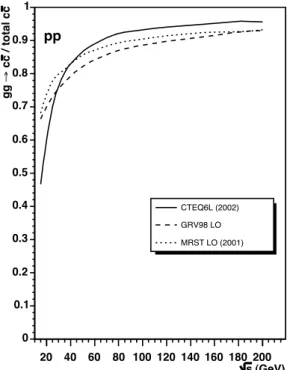
(29) 1. H EAVY QUARKONIUM IN HIGH - ENERGY PHYSICS. 7 TeV LHC parton kinematics 9. 10. WJS2010. x1,2 = (M/7 TeV) exp(±y). 8. 10. Q=M M = 7 TeV. 7. 10. 6. M = 1 TeV. 5. 10. 4. M = 100 GeV. 10. Q. 2. 2. (GeV ). 10. 3. 10. y= 6. 2. 4. 0. 2. 4. 6. 2. 10. M = 10 GeV. 1. fixed target. HERA. 10. 0. 10 -7 10. -6. 10. -5. 10. -4. 10. -3. 10. -2. 10. -1. 10. 0. 10. x (a) plane showing, in blue color, the area that can √ be accessible at the LHC center-of-mass energy s = 7 TeV and for produced resonances with a mass M above 100 GeV (from http://www.hep.phy.cam.ac.uk/~wjs/plots/plots.html).. (Q2 , x). (b) Parton distribution functions inside a proton. The colored curves represent the different partonic contributions (u, d, u, ¯ d,¯ s, c and g) at energy scale Q2 = 10 GeV. The NNLO CT1O(central) parametrization is used for the PDFs (from http://hepdata.cedar.ac.uk).. Figure 1.11. plotted as a function of x, has been evaluated at energy scale Q2 = 10 GeV2 , a value relevant for cc¯ production, according to the NNLO CT1O(central) parametrization. It can be immediately verified that, in the x-ranges we can access, the dominant partonic contribution is the gluon distribution, i.e. at low x-values we mostly find gluons. As a consequence, we can state that quarkonium production at LHC energies mainly proceeds via gluon-gluon interaction (gg → QQ¯ at LO). It is instructive, in relation to the previous statement, to see Fig. 1.12. It shows the relative √ contribution of gluon fusion to the total cc¯ production cross section, as a function of s, as calculated for proton-proton collisions. The remainder of the total cross section is, at leading order, due to qq¯ annihilation. In Fig. 1.12 three different parametrizations (CTEQ6L (2002), GRV98 LO and MRST LO (2001) have been used to describe the parton distributions inside the protons. The contribution from gluon fusion is, already √ for s > 70 GeV, larger than 90 %. ¯ hadroproduction at LHC Once the dominant pQCD process responsible for heavy-quark pair (QQ) energies is known, two points have to be discussed and developed. First of all, concerning the initial perturbative QCD process, we should investigate the main channels (in term of Feynman diagrams) involved in the initial QQ pair creation. Then, the non-perturbative evolution of the QQ pair into a quarkonium state has to be treated in terms of the language of QCD effective theories. Different hypothesis on the perturbative and non-perturbative components lead therefore to var28.

(30) gg ! cc / total cc. 1.2. Quarkonia production in pp collisions 1 0.9. pp. 0.9. 0.8. 0.8. 0.7. 0.7. 0.6. 0.6. 0.5. 0.5. 0.4. CTEQ6L (2002). 0.4. GRV98 LO. 0.3. MRST LO (2001). 0.3. 0.2. 0.2. 0.1. 0.1. 0 20. 40. 60. 80 100 120 140 160 180 200 s (GeV). Figure 1.12. Relative contribution of gluon fusion to the total cc¯ production cross section, as a √ function of s, in pp collisions [41].. ious theoretical models for quarkonium production. Most notable among these are the color-singlet model (CSM), the color-evaporation model (CEM) and the non-relativistic QCD (NRQCD) approach, explained in their main features in the following sections. 1.2.3.3 Color-singlet Model (CSM) The color-singlet model was first proposed shortly after the J/ψ discovery. The central hypothesis of the CSM consists in the assumption that the non-perturbative QQ¯ pair evolution into the quarkonium resonance occurs without any modification of its quantum numbers (spin S, angular-momentum L and color c). Therefore, in order to produce a quarkonium state, the QQ¯ pair must be generated with the quarkonium quantum numbers, and, in particular, the pair has to be created in a color-singlet state (c=1). This explains the name Color-single Model (CSM). The non-perturbative evolution of the QQ¯ pair, which involves the non-perturbative transition | QQ¯ ( 2S+1 LJc=1 ) > → | ψ ( 2S+1 LJc=1 ) >,. (1.25). occurs via emission of low energy (soft) gluons. The total cross section of the partonic process a + b → ψ + X can be derived under two important approximations. The first one concerns the so-called factorization theorem. As already mentioned in Section 1.2.3.1, if one assumes that the quarkonium production can be decomposed in two steps clearly separated in time, first the creation of the heavy-quark QQ¯ pair and then their binding to make the meson, the total cross section can, consequently, be factored into two components. In the second approximation, the velocity of the heavy-quarks (charm and bottom quarks) in the meson is assumed to be negligible. We can therefore suppose that the quarkonium resonances are created with their two constituent quarks at rest in the meson reference frame. This is known as static approximation. 29.

(31) 1. H EAVY QUARKONIUM IN HIGH - ENERGY PHYSICS In the end, the total cross section of the process a + b → ψ + X can be expressed as σˆ (a + b → | ψ ( 2S+1 LJc=1 ) > +X) = σˆ pQCD (a + b →. | cc¯ ( 2S+1 LJc=1 ). � � l � d ψ �2 > +X) × �� l Rnl (0)�� , (1.26) dr. � l � � d ψ �2 (0) R where σˆ pQCD (a + b → | cc¯ ( 2S+1 LJc=1 ) > +X) is the term calculable in pQCD, while � dr � l nl ψ → parametrizes the non-perturbative component. The last term contains the function R (−r ) which nl. is the color-singlet cc¯ wave-function in coordinate space for ψ. The production cross section for each quarkonium resonance ψ is therefore related to the absolute values of the cc¯ wave-function and −r = 0), i.e. zero cc¯ its derivatives (the degree depends on the L value20 ) evaluated at the origin (→ separation. The cc¯ wave-function21 is connected to the amplitude of the transition shown in Eq. 1.25 which cannot be calculated in pQCD being a non-perturbative process. This quantity is therefore extracted from experimental measurements of quarkonium decay rates. Once this extraction has been carried ψ out, the CSM has no other free parameters: for each charmonium state, Rnl (0) is actually the only phenomenological parameter. For what concerns the perturbative term σˆ pQCD (a + b → | cc¯ ( 2S+1 LJc=1 ) > +X), it can be calculated as a perturbative expansion in powers of αs using the standard pQCD methods. The final result is then obtained at a certain order - leading order (LO), next-to-leading order (NLO), next-to-nextto-leading order (NNLO), etc. - by truncating the perturbative series. In the original formulation of CSM, the dominant process is the gluon fusion 22 . Figure 1.13 and 1.14 show representative Feynman diagrams that contribute to the cc¯ hadroproduction, via gluon fusion, at order αs2 and αs3 , respectively.. Figure 1.13. Representative diagrams that contribute to the cc¯ hadroproduction, via gluon fusion, at order αs2 . In more detail, both diagrams shown in Fig. 1.13 can produce pre-resonance cc¯ states in only two quantum number configurations 2S+1 LJ : 1 S0 and 3 PJ . As for the color state, both color-singlet and 20 For. example, l = 0 for S-wave, l = 1 for P-wave, etc. . to the heavy masses of the constituent quarks (charm and bottom), quarkonium spectroscopy can be studied reasonably well in non-relativistic potential theories. The color potential of the QQ¯ system can be represented phenomeno−r ) = σ |→ −r | − α where the second term is the coulombian contribution, logically (at temperature T = 0 K) by the sum V (→ −r | |→ induced by gluon exchange between the quark and the antiquark, while the first term is the confinement one. The colorsinglet QQ¯ wave function can be derived within these non-relativistic static potential theories. 22 Actually, for charmonia produced at high transverse momentum, p � M , the gluon fragmentation results to be the ψ T dominant process. 21 Due. 30.

(32) 1.2. Quarkonia production in pp collisions color-octet are allowed by the two diagrams. Furthermore, within the standard collinear approach, which assumes the initial parton momenta collinear to the proton ones, these diagrams imply that the cc¯ system is created with a transverse momentum pT = 0, due to the 4-momenta conservation. On the contrary, for what concerns the three diagrams shown in Fig. 1.14, only the following quantum number configurations 2S+1 LJ are allowed for the pre-resonance cc¯ states : 1 S0 , 3 S1 ,3 PJ (a), 1 S , 3 P (b) and 1 S , 3 P (c). As previously mentioned, both color-singlet and color-octet states can be 0 J 0 J produced by the three diagrams. Finally, within the standard collinear approach, the three diagrams at order αs3 allow a non-zero transverse momentum pT for the cc¯ system. In fact, the transverse momentum carried by the gluon in the final state counterbalances the pT of the cc¯ pair.. Figure 1.14. Representative diagrams that contribute to the cc¯ hadroproduction, via gluon fusion, at order αs3 . In conclusion, remembering the quantum number configuration for J/ψ (and ψ’) 2S+1 LJ = 3 S1 , we obtain that, in the color-singlet model at leading order (CSM LO), the only diagram which contributes to the direct J/ψ (and ψ’) production is the diagram, at order αs3 , shown in Fig. 1.14 (a). 1.2.3.4 Color-evaporation model (CEM) The color-evaporation model was first introduced at the end of the 70s. Contrary to the CSM, the heavy-quark pair cc¯ is not necessary produced in a color-singlet state. Actually, the CEM does not specify the quantum numbers (spin S, angular-momentum L and color c) of the pre-resonance cc¯ state that can be produced without any constraints on the color or spin of the final state. Therefore, both color-singlet and color-octet states are allowed in the CEM which does not provide the fraction of cc¯ pairs produced in the two color states. In case of cc¯ pairs produced in color-octet state, the CEM assumes that the neutralization of the color occurs via interaction with the collision-induced color field: the exchange of gluons determines a color evaporation which explains the model’s name. The final asymptotic cc¯ state (resonance), in term of spin and color, is therefore randomized by numerous soft interactions occurring during the non-perturbative process of hadronization, and, as a consequence, it is not correlated with the quantum numbers of the cc¯ pair initially produced. As an example of the CEM features, the production of a 3 S1 state (J/ψ, ψ’, ... ) by one gluon is possible, whereas in the CSM it was forbidden by color conservation. The first hypothesis of the color-evaporation model is that the probability for the initial cc¯ pair to evolve into a charmonium state ψ is given by a constant fcc→ψ that is energy-momentum and ¯ probability is therefore an universal constant in any process independent. Within the CEM, the fcc→ψ ¯ √ kinematic region ( s, y, pT ) and for any process (p + p, p + A, π + A, e + p, ... ). In addition, the 31.