HAL Id: hal-01879195
https://hal.archives-ouvertes.fr/hal-01879195v2
Preprint submitted on 21 Feb 2019
HAL is a multi-disciplinary open access
archive for the deposit and dissemination of sci-entific research documents, whether they are pub-lished or not. The documents may come from teaching and research institutions in France or
L’archive ouverte pluridisciplinaire HAL, est destinée au dépôt et à la diffusion de documents scientifiques de niveau recherche, publiés ou non, émanant des établissements d’enseignement et de recherche français ou étrangers, des laboratoires
International Ecolabel Versus National Ecolabels
Amira Bouziri, Hend Ghazzai, Rim Lahmandi-Ayed
To cite this version:
Amira Bouziri, Hend Ghazzai, Rim Lahmandi-Ayed. International Ecolabel Versus National Ecolabels. 2019. �hal-01879195v2�
International Ecolabel Vs National Ecolabels
A. Bouziri
∗a, H. Ghazzai
†band R. Lahmandi-Ayed
‡ca
Mediterranean School of Business and Unité MASE-ESSAI, Université de
Carthage
b
Mediterranean School of Business and Unité MASE-ESSAI, Université de
Carthage
c
ESSAI and Unité MASE-ESSAI, Université de Carthage
∗[email protected] (corresponding author) MSB, Les Jardins du Lac 2, 1053 Tunis,Tunisia †[email protected]
Abstract
We consider a vertically differentiated model with two identical countries each having initially one firm. We compare two options: a unique international ecolabel set up by an international authority and two national ecolabels set up non-cooperatively by two national non-governmental authorities. The governments decide then to open or not their economies, then firms choose their environmental qualities and prices.
We prove that relative to the case of national ecolabels, the international label lets the global welfare as it is or improves it. However, the improvement is always at the expense of one of the two countries, in which case the international label is not feasible unless the beneficiary country offers a compensation to the aggrieved one.
Keywords Environmental quality, international label, national labels, vertical differentiation, welfare.
JEL Classification L11, L13, Q56, Q58.
This paper has not been submitted elswhere in identical or similar form, nor will it be during the first three months of its submission to the Publisher.
1
Introduction
Environmental concerns have become one of the most significant pressures on human de-velopment in recent decades. In this context, with increasing public awareness of products’ environmental quality and the consciousness of the harmful effects of product consumption, policy-makers, firms and consumers are actively considering how to reduce negative effects on environment while consuming and producing. Ecolabels are among the instruments intended to protect the environment. An ecolabel is defined as a logo, symbol, or a proof of autho-rization given to the product that enlightens consumers about better ecological quality and communicates unobservable information about the environmental attributes of goods. It may be voluntarily applied for by firms that wish to display an environmentally friendly image.1
With the consciousness of the effects of human activities on environment, emerges a con-sciousness of the globality of these effects, and the issue of international cooperation re-emerges repeatedly through numerous international conferences, conventions and agreement attempts, for instance: the International Convention on Wetlands (February 1971), the Con-vention on the Conservation of European Wildlife and Natural Habitats (June 1982), the Vi-enna Convention for the Protection of the Ozone Layer (September 1988), the United Nations Framework Convention on Climate Change (March 1994) ratified by 197 countries, the Kyoto Protocol (February 2005) with the objective of reducing greenhouse gas emissions and the Paris Agreement COP21 (November 2016) aiming at fighting climate change for all countries by assisting developing ones.
Concerning ecolabels, one issue of interest is to know whether the international coop-eration in terms of ecolabels is relevant and feasible. Precisely, the aim of this paper is to investigate whether the set-up of a unique international ecolabel by an international authority improves the global welfare relative to national ecolabels set up non-cooperatively by national authorities, and to what extent countries would support such an initiative.
international component assuming the existence of two countries with one firm in each coun-try initially producing a low environmental quality. We consider two procedures of ecolabels’ set-up. In the first one (centralized or international label case), countries cooperate and create a supra-national labeling authority in charge of choosing a unique international label. The objec-tive of the international authority is to maximize the global welfare. Then, governments decide non-cooperatively whether to open or close their frontiers. Finally, firms choose either to be labeled or not and then compete in prices. In the second case (decentralized or national labels case), we assume that two national non-governmental labeling authorities exist, one in each country. The authorities choose non-cooperatively the levels of labeling criteria. The objective of each national authority is to maximize the welfare of its own country. Then, governments decide whether to open or close their frontiers. Finally, firms choose to be labeled or not prior to competition in prices. When a firm chooses to be ecolabeled, it incurs a fixed cost increasing with the difference between the label quality and the initial one. The marginal production cost is moreover assumed to be increasing with respect to quality.
Our main results reveal three important outcomes. First, countries prefer openness to au-tarky in either the international and the national labels cases for low values of the marginal production costs. Second, the global welfare with an international label is higher than or equal to the global welfare with national labels. When an international label improves the global welfare, it is always at the expense of one of the two countries which is thus expected to op-pose the international label program.
The related literature: Different definitions have been adopted when modeling ecolabels. In some papers, like in our model, a firm obtains an ecolabel if it meets a high enough standard (Li & Van’t Veld, 2015; Fischer & Lyon, 2014; BenYoussef & Abderrazak, 2009; BenYoussef & Lahmandi-Ayed, 2008; Nimon & Beghin, 1999). In other papers, firms obtain a label when they choose a "green" technology. In Ibanez & Grolleau (2008) and Hamilton & Zilberman (2006), firms have the choice between two types of technologies: conventional or "green". In Amacher et al. (2004), a label is awarded to a firm if it makes positive investments in a "green"
technology, no matter how small these investments are. In Greaker (2006), firms obtain a la-bel if their emissions per unit produced does not exceed a certain level specified by the lala-bel. Finally, in Tian (2003), the label is a sticker indicating the exact level of environmental friend-liness of a product.
Producing a "green" product increases firms’ costs. In Fischer & Lyon (2014), only the variable costs are affected. In Hamilton & Zilberman (2006) and Rothfels (2002), only fixed costs increase. In our paper and in most of the papers dealing with "green" products, both the variable and fixed costs increase. Amacher et al. (2004) is the only paper assuming that ob-taining an ecolabel increases the fixed costs but decreases the variables costs.
Consumers’ preferences are positively affected by the level of environmental friendliness of a product. This is what is referred to in the literature as the warm glow effect which rep-resents the private benefit from consuming a certain environmental quality. As in our paper, many papers only consider this effect when modeling consumers’ preferences (Li & Van’t Veld, 2015; Fischer & Lyon, 2014; Andre et al., 2009; Rothfels, 2002). Consumers’ prefer-ences may also be negatively affected by pollution which is either represented by the aggregate consumption of other consumers as in Tian (2003) or by the emission of firms as in Greaker (2006) or by the average environmental quality of all products in the market as in Amacher et al. (2004).
Different issues have been studied when considering "green" markets and ecolabels. We can classify these issues into five streams: (1) Firms’ incentives to adopt environmentally friendly products (2) effects of environmental policies on international trade (3) implication of imperfect monitoring of ecolabels (4) perverse effects of ecolabels and (5) competition be-tween ecolabels. Our paper belongs to the first and second streams.2
From the first stream, we may cite Amacher et al. (2004), BenYoussef & Lahmandi-Ayed (2008), and Andre et al. (2009). Amacher et al. (2004) prove that firms’ incentives to invest in
a green technology (and consequently to obtain an ecolabel) depend on their relative cost struc-ture. Amacher et al. (2004)’s model completely dissociates the environmental quality provided by a firm from its investment decision as it allows a labeled firm to produce a low environmen-tal quality. It seems more appropriate to assume that firms obtain a label when they produce a high ecological quality as we do in our paper.
The model studied by Andre et al. (2009) is similar to ours. Indeed, they also consider a duopoly model of vertical product differentiation in which two firms first simultaneously choose between two environmental qualities then set prices. The main difference is that at the price stage of the game, they allow firms to cooperate, set the same price and get nonneg-ative profits when they produce the same quality. Moreover, they examine the implication of taxing the low quality firm. Finally, the quality of the "green" product is endogenous in our model while it is exogenous in Andre et al. (2009).
BenYoussef & Lahmandi-Ayed (2008) use a vertical differentiation model with a central au-thority and two identical firms. A central auau-thority chooses first the level of labeling criteria such that the social surplus is maximized, then firms compete in environmental qualities and prices. We extend the model of BenYoussef & Lahmandi-Ayed (2008) to the international con-text considering two countries with one firm in each one. As in BenYoussef & Lahmandi-Ayed (2008), the labeling criteria are determined endogenously in an international framework.
Many papers consider differentiation models when studying the effects of environmental policies on international trade. Different environmental policies are studied. Nimon & Beghin (1999) study the effect of ecolabels in the textile and apparel market when exogenous ecola-bels can be set by a developed country and a developing one. Three situations are compared: no label, a unique label exists in the developed country and two labels exist, one in each coun-try. The comparison is made for specific values of the qualities of the labeled and non labeled products and the costs, which may question the generalization of the results. Greaker (2006) compares the choice of a minimum environmental standard to the set-up of an ecolabel. He shows that it may be optimal for the domestic government to introduce an ecolabel and get both firms to adopt the label, instead of setting an environmental standard. Rothfels (2002)
analyzes the impact of two environmental policies: a minimum quality standard and subsi-dization of the production costs. Assuming that initially the domestic industry lags behind, the paper investigates the possibility that the domestic firm produces a higher quality after regula-tion than that of the competitor prior to regularegula-tion. Finally, Tian (2003) studies the effects of imposing a minimum standard on imported goods. It is shown that an increase in the minimum required level of environmental friendliness of imported goods may harm the home firm. In all the papers mentioned above, economies are always assumed to be open and the reasoning is made mainly from the perspective of the domestic country. In our paper, the decision of a country to open or close its frontiers is endogenous to the model and we are interested in the global effect of ecolabels.
The remaining of the paper is structured as follows. Section 2 presents the model and pre-liminary calculations. Section 3 is devoted to results. We conclude in Section 4. Appendix A provides the notations. Appendices B, C and D contain the proofs of the results obtained respectively in the international label case, the national labels case and for the comparison between the two cases.
2
The Model and Preliminary Calculations
We begin by providing the model then we present some preliminary calculations which will be helpful for further developments.
2.1
The model
Our model is based on BenYoussef & Lahmandi-Ayed (2008)’s model. We suppose that the world is restricted to two countries (i = 1, 2). Countries have identical populations of con-sumers and have each one Firm i. Governments in each country have the choice between opening their frontiers or not. Autarky (O) corresponds to the situation where at least one gov-ernment chooses to close its frontiers in which case each firm is a monopoly in its own country. The open economy case (O) prevails when both governments choose to open their frontiers,
then, each firm sells its product in both countries. When only one government opens its econ-omy, it has no effect and autarky prevails.
We assume that consumers are aware of the need of preserving the environment for current and future generations. This consciousness is tackled through their preference for the most environmental friendly product if they have the choice between several environmental qualities offered at the same price. In each country i, consumers are characterized by their intensity of preference for the environmental quality denoted by θ and are uniformly distributed over the interval [θ, θ], with 0 < θ < θ. We assume that each consumer buys exactly one unit of the product from the firm which ensures to him/her the highest utility. As in Mussa & Rosen (1978), the indirect utility of a consumer θ buying quality qi at price pi, is given by:
ui(θ)= θqi− pi.
Denote by y the highest price consumers are willing to pay for the product. Price y is supposed to be sufficiently high so as it is never constraining.
As the environmental quality is difficult to observe by a simple consumer, the set-up of an ecolabel aims at providing consumers with a partial information about the environmental qual-ity of a product. The attribution of an ecolabel to a firm means that the environmental qualqual-ity of the firm exceeds some given threshold ˜q, called in the following labeling criteria. Hence as far as consumers are concerned, if Firm i is labeled then it has a priori a quality qi ≥ ˜q and a
non-labeled one has a quality qi < ˜q.
Production of some quality q is characterized by a constant marginal cost c(q) = αq with α ≥ 0. The marginal cost c(q) is then assumed to be an increasing function with respect to q as environment friendly processes are supposed to be more costly.
produce a quality better than q as it is more costly and not recognized by consumers. Once an ecolabel is set up, the preceding hypotheses imply that it is never profitable for firms to pro-duce a quality different from q and ˜q. The choices of firms are thus consistent with consumers’ beliefs. Indeed as consumers are not able to make the difference between q and a quality q satisfying q ≤ q < ˜q and between ˜q and a better quality, producers try to set the product in "some category" (labeled or not labeled) at the least cost.
Moving to a quality ˜q involves a fixed cost I increasing with respect to the difference between the initial and the new quality assumed to be given by:
I(∆˜q) = β(∆˜q)2
with β > 0 and∆˜q = ˜q − q.
We assume that each unit consumed involves a damage d. The unit damage3 is supposed to be decreasing with quality at a constant rate µ > 0. Formally, we assume that:
d = γ − µq
with γ > 0.
Parameter µ measures the negative slope of the damage with respect to the environmental quality. The higher µ the faster the damage decreases with the environmental quality. We may then refer to µ as the environmental sensitivity to quality.
Parameter γ refers to the maximal environmental damage occurring in the case of a null quality.
We consider two scenarii which differ by the way the labeling criteria are chosen: the in-ternational and the national labels cases to be described below.
International Label Case
In this case, the label is set up by a supra-national authority in a centralized way and the game is organized as follows:
1. The supra-national authority chooses a unique level of labeling criteria ˜q so as to maxi-mize the global welfare.
2. Governments of both countries choose simultaneously and non-cooperatively whether to open(O) or close (O) their economies so as to maximize the governments’ welfare.
3. Firms choose simultaneously their qualities qiin the pair {q, ˜q}.
4. Firms choose simultaneously their prices in [0, y].
The global welfare to be maximized in the first step corresponds to the sum of consumers’ and producers’ surpluses in both countries minus the environmental damage caused by the con-sumption of goods. As far as the governments try generally to "please" the current generation, they take the environment issue into consideration only through consumers’ surpluses. The government’s welfare to be maximized at the second step is equal to the sum of firm’s profit and consumers’ surplus, without considering the environmental damage.
National Labels Case
In this case, two labels are set up by two national non-governmental authorities, in a decen-tralized way. The game is organized as follows:
1. National non-governmental authorities choose, simultaneously and non-cooperatively, the level of labeling criteria ˜qi so as to maximize the countries’ welfares.
2. Governments in each country choose simultaneously whether to open (O) or close (O) their economies.
3. Firms choose simultaneously their qualities. Each firm i chooses its quality qiin the pair
{q, ˜qi}.
4. Firms choose simultaneously their prices in [0, y].
The country’s welfare to be maximized in the first step equals the sum of consumers’ and producers’ surpluses in each country minus the environmental damage caused by the con-sumption of goods in that country. The government’s welfare maximized in the second step is supposed equal to the sum of the firm’s profit and consumers’ surplus. Although the authority is national, it acts independently of the government and does not have the same objective as the latter. While a labeling authority cares about the environmental damage, we assume that governments take their decisions by only considering consumers’ and firms’ interests.
We also assume that a firm can only adopt the label of the authority of its own country. This is observed in real life for many national ecolabels. Although there may be no specific condition on the nationality of the firms that may apply for the label, technically, the procedure of labels’ adoption is tedious and long and makes it very difficult for foreign firms to adopt the label.
As proven in Appendices B and C, multiple equilibria may exist at the quality stage of the game. When needed we adopt the following selection assumption.
(SA): If multiple equilibria exist, we choose the equilibrium where firms produce the high-est pair of qualities.
Multiple equilibria may occur at the quality stage of the game in both the international label and the national labels cases. With the selection assumption (SA), we ensure that the re-sulting environmental damage is the lowest possible. For some values of the labeling criteria, a firm has the same profit with the labeled product and the non-labeled one. With assumption (SA), it chooses to produce the labeled one. Like consumers, firms are someway supposed to
have an ecological consciousness.
Finally, it is worth noting here that the international label case is not equivalent to the co-operative version of the national labels one. In the coco-operative version of the national labels case, the two national labeling authorities choose cooperatively the levels of the national label-ing criteria ˜q1 and ˜q2so as to maximize the sum of their surpluses anticipating the following
steps of the national game. Whereas in the international label case only one authority exists and maximizes the global welfare with respect to a unique level of labeling criteria ˜q and both firms can choose between q and ˜q.
2.2
Preliminary results
We need for both cases (i.e. International label and National labels) the output of the Autarky case and the price equilibrium in the open economy case for two given qualities.
In Autarky, Firm i is a monopoly in its own country. The equilibrium outcome is described in Result 1. When economies are open, Result 2 provides the price equilibrium.
Result 1. In Autarky, the monopoly does not get the label. It produces qm= q at price pm = y
making a profitΠ= (y − αq)(θ − θ). The social welfare in each country is then given by:
S W = (θ − θ)[q(θ+θ2 −µ − α) + γ].
In the absence of competitors, the monopoly has no incentive to adopt the label as it can set the highest possible price y for the lowest quality q and serve all consumers without incurring the extra-costs of producing a labeled product.
Result 2. When economies are open, denote by qi and qj the qualities sold respectively by
Firms i and j in both countries.
• If qi = qj = q. Firms share equitably the market, set prices pi = pj = αq.
– ifα ≥ 2θ − θ, only the low quality firm is active and prices are given by pi = αqi, pj = αqi−θ(qi− qj).
– ifα ≤ 2θ − θ, only the high quality firm is active and prices are given by pi = αqj+ θ(qi− qj), pj = αqj.
– if 2θ − θ < α < 2θ − θ, both firms are active and prices are given by
pi = 13[(2θ − θ)(qi− qj)+ 2αqi+ αqj], pj = 13[(θ − 2θ)(qi− qj)+ αqi+ 2αqj].
3
Results
In this section, we provide the equilibrium outcome of the international label case, then those of the national labels one and finally we compare the outcomes of the two scenarii. Before that, we enounce a result on the activity of a label common to both scenarii. By active label, we mean a label adopted by at least one active firm.
Denote by: δL = 2(θ−θ)(θ−α) β , δI = 9β2(2θ − θ − α)2, ˆ δ = 13(θ−α)2−8(θ−α)2+(θ−θ)2 18β .
Result 3 (Activity of a Label). A label with given labeling criteria ˜q is active if and only if {α < 2θ − θ and∆˜q ≤ δL} or {2θ − θ < α < 2θ − θ and∆˜q ≤ min{δI, ˆδ}}.
Result 3 is a corollary of Lemmas 1 to 4 in Appendices B and C. A label is never active when α > 2θ − θ as the variable production cost of the labeled product is too high. There is no
room for a labeled firm even in the absence of fixed labeling costs.
Taking into account the investment required to produce a labeled product, two conditions must be satisfied for the labeled firm to be active. First, countries must be open, which is always the case when α < 2θ − θ, but requires∆˜q ≤ ˆδ for 2θ − θ < α < 2θ − θ. Second, the profit of the labeled firm must be nonnegative, which implies that∆˜q ≤ δL for α < 2θ − θ and∆˜q ≤ δI for
2θ − θ < α < 2θ − θ.
The effect of opening the frontiers on the surplus of the government of the country of the labeled firm is not obvious. The firm is a monopoly in Autarky and makes positive profits but consumers have the lowest surplus. When economies are open, the labeled firm faces compe-tition. It has access to a bigger market but has higher costs. Consumers have a higher surplus. Condition∆˜q ≤ ˆδ ensures that the surplus of the government of the country of the labeled firm is higher than its surplus in Autarky when 2θ − θ < α < 2θ − θ.
It is also worth noting that the activity of the label is a necessary condition for governments to open their frontiers. In fact, if no label is active, governments have the same surplus whether economies are closed or open.
3.1
The International Label Case
In this subsection, we determine the equilibrium outcome of the international label case in terms of qualities, decision to open or not the economy and the level of the labeling crite-ria. The international label game is solved by backward induction. The price equilibrium has already been given in Results 1 and 2. Now, we calculate the equilibrium qualities then we specify conditions under which economies will be open. Finally, we determine the optimal labeling criteria of the international label. The outcome of the Subgame Perfect Nash equi-librium in the international label case is summarized in Proposition 1. A detailed proof is provided in Appendix B.
MC1 = (5 − 3 √ 3)θ − (4 − 3√3)θ, MC2 = (13−3 √ 3 5 )θ − ( 8−3 √ 11 5 )θ, δ∗c L = (θ−θ)(θ+θ−2α+2µ) 2β , δ∗c I = (2θ−θ−α)(4θ+θ−5α+6µ) 18β . δ∗c L and δ ∗c
I are the levels of the labeling criteria that maximize the social welfare without
constraint respectively in the case of low marginal costs and intermediate marginal costs (i.e. the condition on the activity of a label is not binding). These two levels are increasing with respect to µ, as the higher is the impact on the environment, the more stringent will be the labeling criteria.
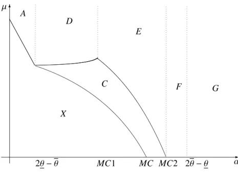
Proposition 1 (The International Label Case). The outcome at the subgame perfect equilib-rium in the international label case is provided in Table 1 and depicted in Figure 1.
Zone α µ Qualities labeling criteria: ˜q∗ Openness/ Autarky 1 α ≤ (2θ − θ) µ > 3θ−θ2 −α (δL+ q, q) δL+ q 2 α ≤ (2θ − θ) µ ≤ 3θ−θ2 −α (δ∗cL + q, q) δ∗cL + q 3 (2θ − θ) < α < MC1 µ > α−5θ+4θ6 (δI + q, q) δI+ q 4 (2θ − θ) < α < MC1 µ ≤ α−5θ+4θ6 (δ∗cI + q, q) δ∗cI + q Openness MC1< α < (θ+θ) 2 µ ≤ (θ−θ)(θ+θ−2α) 2θ−θ−α 5 MC1< α < (θ+θ) 2 µ > (θ−θ)(θ+θ−2α) 2θ−θ−α (ˆδ+ q, q) δ + qˆ θ+θ 2 < α < MC2 µ ≥ 0 6 MC2 < α < (2θ − θ) µ ≥ 0 (q, q) Any ˜q in [q, q] Autarky
7 α > (2θ − θ) µ ≥ 0 (q, q) Any ˜q in [q, q] Indifference
Table 1 – Equilibrium outcomes in the International Label case
The outcome of the game depends on the marginal cost α and the environmental sensitivity to quality µ. Seven zones appear in the international label case. In zones 1 to 5, economies are open, one firm adopts the label and the other firm produces or proposes the non-labeled product. In zones 6 and 7, no firm adopts the label.
-6 1 2 3 4 5 4 6 7 µ α 2θ − θ MC1 θ+θ 2 MC2 2θ − θ
Figure 1 – International label case
Increasing the labeling criteria does not have an obvious impact on the global welfare. It affects positively the environment as it reduces the environmental damage. It also increases consumers’ satisfaction as they have the opportunity to buy a higher quality. At the same time, it relaxes price competition between firms, which allows them to set higher prices and there-fore negatively affects consumers’ surplus. Finally, it increases the production and investment costs of the labeled firm, which has a negative effect on its profit. It may even lead the firms to completely ignore the label when the costs are too high. The outcome of the game can be interpreted from two different perspectives: the resulting environmental improvement and the resulting global welfare.
When considering the environmental improvement, three areas appear:
Complete environmental improvement: This area corresponds to zones 1 and 2 where the marginal cost is low. As only the labeled firm is active at the price stage of the game, only the labeled product is sold and the environmental improvement is maximal.
Partial environmental improvement: This area corresponds to zones 3, 4 and 5 where the marginal cost is intermediate. As both the labeled and the non-labeled firms are active at the price stage of the game, the labeled product is sold only to consumers with high preferences for the environmental quality, the other consumers buying a low quality product.
No environmental improvement:This area corresponds to zones 6 and 7. As the marginal cost is very high, no firm adopts the label. In zone 6, the label is ignored and Autarky prevails. Governments are better off closing their frontiers. In zone 7, marginal costs are very high and producing a high quality is too costly. No firm adopts the label whether economies are open or closed and countries have exactly the same welfare whether economies are open or closed.
From the perspective of the global welfare, we also identify three areas:
Unconstrained global welfare: This area corresponds to zones 2 and 4 where both the marginal cost α and the environmental sensitivity to quality µ are low.4In this area, the level of the
label-ing criteria corresponds to the one that maximizes the global welfare without constraints. As both the marginal production cost and the the environmental sensitivity to quality are low, the labeling criteria need not be very severe i.e. not very high. Thus, both the variable production costs of the labeled product and the fixed investment costs of moving to a labeled product are not very high. The labeled firm will make a positive profit and the country of the labeled firm is better off than under Autarky.
Constrained global welfare: This area corresponds to zones 1, 3 and 5 where the marginal cost is low but the environmental sensitivity to quality is high. The high environmental sensitivity to quality leads to high labeling criteria and one of the conditions for a label to be active is binding. In zones 1 and 3, the binding constraint is the one ensuring nonnegative profit for the labeled firm (∆˜q ≤ δL in zone 1 and∆˜q ≤ δI in zone 3). At equilibrium, the labeled firm will
make a null profit, which means that∆˜q = δLin zone 1 and ∆˜q = δI in zone 3. In zone 5, the
binding constraint is the one ensuring the openness of the economies (∆˜q∗ ≤ ˆδ). At
equilib-rium, the active label is the highest ensuring it (∆˜q∗ = ˆδ). The government of the country of the labeled firm has the same welfare as in the Autarky case.
Autarky global welfare: This area corresponds to zones 6 and 7 where firms completely ignore the label.
3.2
The National Labels Case
In this paragraph, we determine the equilibrium outcome of the National Labels case in terms of qualities, decision to open or not the economy and labeling criteria. Denote by:
MC = 16θ−11θ5 + √ 171 5 (θ − θ), δ∗d I = ˆ δ 2+ 1 6βµ(2θ − θ − α), µ1 = 4(θ−θ)(θ+θ) (2θ−θ−α) − 3βˆδ 2θ−θ−α , µ2 = 43(2θ − θ − α) − 2θ−θ−α3βˆδ . δ∗d
I is the level of the labeling criteria that maximizes the social welfare of the country of the
labeled firm without constraint in the case of intermediate marginal costs (i.e. the conditions on the activity of the label are not binding). It is increasing with respect to µ as the higher is the impact on the environment of the quality, the more stringent will be the labeling criteria. MC1, MC2, δL, δIand ˆδ have the same expressions given previously.
Proposition 2 provides the equilibrium outcome of the national labels case.
Proposition 2 (The National Labels Case). The outcome at the Subgame Perfect Equilibrium in the national labels case is provided in Table 2 and depicted in Figure 2.
Zone α µ Qualities Active Label Criteria: ˜q∗ Openness/ Autarky
X α ≤ (2θ − θ) µ ≤5θ−θ−4α2 No equilibrium No equilibrium (2θ − θ) < α < MC µ ≤ µ1 A α ≤ (2θ − θ) µ >5θ−θ−4α2 (δL+ q, q) δL+ q C (2θ − θ) < α < MC1 µ1< µ < µ2 MC1< α < MC µ1< µ < 3βb δ 2θ−θ−α (δ ∗d I + q, q) δ ∗d I + q Openness MC< α < MC2 µ < 3βb δ 2θ−θ−α D (2θ − θ) < α < MC1 µ > µ2 (δI+ q, q) δI+ q E MC1< α < MC2 µ >(2θ−θ−α)3βbδ (ˆδ+ q, q) δ + qˆ F MC2< α < (2θ − θ) µ ≥ 0 (q, q) Any ˜q in [q, q] Autarky
G α > (2θ − θ) µ ≥ 0 (q, q) Any ˜q in [q, q] Indifference
-6 µ α 2θ − θ MC1 MC MC2 2θ − θ X A D E F G C
Figure 2 – National labels case
Similarly to the international case, the outcome of the game depends on the marginal cost α and the environmental sensitivity to quality µ. Eight zones appear in the national labels case. In zones A, C, D and E, only one firm adopts the label and the other firm produces or proposes the non-labeled product. In zones F and G, no firm adopts the label. In zone X, there is no equilibrium at the labeling criteria stage of the game. We first notice that in all zones, at most one label will be active i.e. at most one label will be adopted. This situation corresponds to the outcome of a standard vertical differentiation model where maximal differentiation occurs. As in the international label case, the outcome of the game can be interpreted from two different perspectives: the resulting environmental improvement and the resulting welfare of the coun-try of the labeled firm.
From the perspective of the environmental improvement, as in the international case, the environmental improvement is maximal for low marginal costs (Zone A), partial for interme-diate marginal costs (Zones C, D and E) and there is no environmental improvement when marginal costs are high (Zones F and G). The main qualitative difference between the interna-tional label case and the nainterna-tional labels case is the existence of zone X where no equilibrium exists at the labeling criteria stage.
From the perspective of the welfare of the country of the labeled firm, the above mentioned zones can be classified in 4 main areas:
Unconstrained welfare of the country of the labeled firm:it corresponds to zone C. The con-ditions for a label to be active are not binding in this zone. The level of the labeling criteria is the one that maximizes the welfare of the country of the labeled product without constraint. As the environmental sensitivity to quality is low, the labeling criteria need not be very severe. The marginal cost is intermediate. Thus, the production costs and the investment costs are not very high and the labeled firm will make positive profits. The country of the labeled firm and its government are better off than under Autarky.
Constrained welfare of the country of the labeled firm: it corresponds to zones A, D and E where the marginal cost is low but the environmental sensitivity to quality is high. A high en-vironmental sensitivity to quality leads to severe labeling criteria. As in the international case, one of the conditions for a label to be active is binding. The binding constraint is∆˜q ≤ δLin
zone A and∆˜q ≤ δI in zone D and therefore the labeled firm will make a null profit. In zone
E, the active label is the highest that ensures economies be open.
Autarky Welfare:it corresponds to zones F and G. In zone F, autarky prevails. In fact, if a firm chooses to be labeled, the surplus of its government will be lower than under a closed econ-omy. In zone G, marginal costs are very high and producing a high quality is too costly. No firm will adopt the label. Countries have exactly the same welfare whether the economies are open or closed.
Instability: it occurs for a low marginal cost and a low environmental sensitivity to quality rate (Zone X). Economies are open in this area and no equilibrium exists at the labeling crite-ria stage of the game. In fact, as being labeled implies neither high production costs nor high investment costs, competition between authorities at the label stage is too fierce. There is al-ways a profitable deviation by one of the authorities that makes her label active. This leads to an unstable situation, as authorities will keep changing their labeling criteria and consequently firms will keep changing the qualities they offer.
3.3
Comparison: International Label Vs National Labels
In this section, we compare the outcomes of the international label and the national labels cases from the viewpoint of the global welfare and the viewpoint of each country. As different outcomes result in both cases, the question is whether the creation of an international authority in order to set up a unique ecolabel improves the global welfare relative to the national labels case, and if so whether this improvement means the improvement for each country.
Proposition 3 coupled with Figure 3 summarize the main results of the comparison.
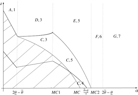
Proposition 3 (Comparison). Comparing the international label and national labels outcomes and given the zones defined in Figure 3, we have,
• In zones (A,1), (D,3), (E,5), (F,6) and (G,7), the international label and the national labels cases lead to the same outcome.
• In zones (C,3), (C,4) and (C,5), relative to the case of national labels, the international label improves the global welfare, improves the welfare of the country of the non-labeled firm and deteriorates the welfare of the country of the labeled firm.
• In the hatched zone, the national labels case leads to an unstable situation with no equilibrium. Whereas, the international label case always has an equilibrium at the label stage of the game.
Our first result is that the global welfare with an international label is the same as the global welfare with national labels in zones (A,1), (D,3), (E,4), (F,6) and (G,7). In these zones, the set-up of an international label has no effect relative to national labels. This occurs for a high marginal cost or a high environmental sensitivity to quality. Knowing that the set-up of a supra-national authority requires some costs (fixed and variable)5, no matter how low are the costs, there is no point in this case to set up a unique ecolabel.
The global welfare with an international label is strictly higher in zones (C,3), (C,4), and (C,5) where it seems relevant to set up a unique international label.
In the hatched zone, the set-up of an international label solves the instability problem ob-served with national labels. Therefore, it may be relevant in this case i.e. for low marginal costs
6 µ α 2θ − θ MC1 MC MC2 2θ − θ -θ+θ 2 A, 1 D, 3 C, 3 C, 5 C, 4 F, 6 E, 5 G, 7 # # #
Figure 3 – International label Vs National labels
and low environmental sensitivity to quality to establish a supra-national authority.
Coming to the viewpoint of countries, we compare the welfare of each country (i.e. country of the labeled firm and country of the non-labeled firm) in the two cases: the international label case and the national labels case. Relative to the national labels case, setting up a unique inter-national ecolabel improves the welfare of the non-labeled firm’s country or lets it unchanged. However, the welfare of the country of the labeled firm may decrease with an international label, more precisely in zones (C,3), (C,4) and (C,5). This happens, as in zone C, the level of the labeling criteria in the national labels case corresponds to the one that maximizes the global welfare of the country of the labeled firm without constraint. In this case, this country prefers the situation where each labeling authority chooses non-cooperatively its label. As we reasonably suppose the necessity of cooperation of both countries to set up a unique interna-tional ecolabel, it is likely that the aggrieved country will prevent such an agreement unless it may benefit from a compensation from the beneficiary country. The amount of the compensa-tion for the labeled firm’s country (i.e. the aggrieved country) is equal at least to the difference between its social welfare in the national labels case and its welfare in the international label one. This difference depends on the zones. The amount of the minimal compensation is given in Appendix D at the end of the proof of Proposition 3.
4
Conclusion
We consider a vertically differentiated model where the ecological labeling criteria and gov-ernments’ decision to open internationally are endogenous. Two scenarii are considered. In the international label case, there is a supra-national authority in charge of fixing the labeling criteria of a unique international ecolabel while maximizing the global welfare. In the national labels case, we assume that there are two labeling authorities, one in each country, that choose non-cooperatively their countries’ ecolabels.
Our results concerning the benefits and the feasibility of international cooperation to estab-lish a unique ecolabel lead to different conclusions depending on the environmental sensitivity to quality and the marginal production cost. It turns out that the set-up of a unique international ecolabel by a supra-national authority is not always relevant. When the marginal cost is high or the environmental sensitivity to quality is high, an international label does not improve the global welfare, which questions its relevance. Keeping in mind that the international option requires some costs to set up a supra-national authority, no matter how low these costs are, the set-up of an international label is never relevant if it does not improve the global welfare. The international label is relevant when both the marginal cost and the environmental sensitiv-ity to qualsensitiv-ity are low. It allows to reach a stable situation contrary to the national labels case where no equilibrium is reached at the labeling criteria stage of the game.
When a unique international ecolabel improves the global welfare, the improvement is always at the expense of one of the two countries which may thus oppose the international option. In other words, when the international ecolabel is relevant, it is feasible only if a compensation mechanism is set up in favor of the aggrieved country.
There are many ways to extend our research. First, the decision of governments to open their economies requires that both agree on doing so. We may consider the situation where one government can decide unilaterally to open its frontiers i.e the government may allow foreign firms to sell their products on its market independently of the decision of the other country. Second, we considered in this paper the damage per unit consumed. We justify this assumption
by the importance of pollution and greenhouse emissions coming from some products’ con-sumption (e.g. cars, electronic materials, plastic bags, packaging...). It would be interesting to study environmental damage caused by production. Finally, we may consider the situation where both the international label and the national labels co-exist.
Notes
1Some Examples of ecolabels: NF Environnement, EU Ecolabel, Energy Star, Blue Angel...
2See Ibanez & Grolleau (2008) and Hamilton & Zilberman (2006) for the implication of imperfect monitoring
of the label, Mattoo & Singh (1994) and Dosi & Moretto (2001) for the possible undesirable and perverse effects of ecolabeling and Harbaugh et al. (2011), BenYoussef & Abderrazak (2009), Fischer & Lyon (2014) and Li & Van’t Veld (2015) for the competition between ecolabels.
3The damage considered in this paper is a damage due to the consumption of the product in the country. We
may have considered the damage due to production. This is justified for a variety of products such as cars, plastic bags, electronic material for which the pollution and greenhouse emissions resulting from consumption are by far more important than the pollution resulting from production.
4 By unconstrained global welfare, we refer to the situation where the conditions for a label to be active are
not binding.
References
Amacher F S, Koskela E, Ollikainen M (2004) Environmental quality competition and eco-labeling. Journal of Environmental Economics and Management 47(2): 284-306.
Andre F J, Gonzalez P, Porteiro (2009) Strategic quality competition and the Porter Hypothe-sis. Journal of Environmental Economics and Management 57(2): 182-194.
Bagnoli M, Watts S (2003) Selling to socially responsible consumers: Competition and the private provision of public goods. Journal of Economics and Management Strategy 12(3): 419-445.
BenYoussef A, Lahmandi-Ayed R (2008) Eco-labeling, competition and environment: Endog-enization of labeling criteria. Environmental and Resource Economics 41(2): 133-154.
BenYoussef A, Abderrazak C (2009) Multiplicity of eco-labels, competition, and the environ-ment. Journal of Agricultural and Food Industrial Organization 7(2): 1-22.
Dosi C, Moretto M (2001) Is ecolabeling a reliable environmental policy measure? Environ-mental and Resource Economics 18(1): 113-127.
Fischer C, Lyon T P (2014) Competing environmental labels. Journal of economics and man-agement strategy 23(3): 692-716.
Galarraga Gallastegui I (2002) The use of eco-labels: a review of the literature. European Environment 12(6): 316-331.
Greaker M (2006) labels, Trade and Protectionism. Environmental and Ressource Eco-nomics 33: 1-37.
Hamilton S F, Zilberman D (2006) Green markets, eco-certification, and equilibrium fraud. Journal of environmental economics and management 52(3): 627-644.
Harbaugh R, Maxwell J, Roussillon B (2011) Label confusion: The Groucho effect of uncertain standards. Management Science 57(9): 1512-1527.
Ibanez L, Grolleau G (2008) Can eco-labeling schemes preserve the environment? Environ-mental and resource economics 40(2): 233-249.
Jha V, Vossenaar R, Zarrilli S (1997) Eco-labelling and international trade. Springer.
Li Y, Van’t Veld K (2015) Green, greener, greenest: Eco-label degradation and competition. Journal of environmental economics and management 72: 164-176.
Mattoo A, Singh H V (1994) Eco-labeling: Policy consoderations. Journal of economic theory 41(1): 53-65.
Mussa M, Rosen S (1978) Monopoly and product quality. Kyklos 18(2): 301-317.
Nimon W, Beghin J (1999) Ecolabels and International Trade in the Textile and Apparel Mar-ket. American Journal of Agricultural Economics 81(5): 1078-1083.
Rothfels J (2002) Environmental policy under product differentiation and asymmetric costs: Does leapfrogging occur and is it worth it? In: Marsiliani L, Rauscher M, Withagen C (eds) Environmental Economics and the International Economy. Economy and Environment, vol 25. Springer, Dordrecht.
Tian H (2003) Eco-labeling scheme, environmental protection, and protectionism. The Cana-dian Journal of Economics 36(3): 608-633.
Appendix A: Notations
Notation Value δ∗c L (θ−θ)(θ+θ−2α+2µ) 2β δL 2(θ−θ)(θ−α) β δ∗c I (2θ−θ−α)(4θ+θ−5α+6µ) 18β δ∗d I ˆ δ 2+ 1 6βµ(2θ − θ − α) δI 9β2(2θ − θ − α)2 ˆ δ 13(θ−α)2−8(θ−α)2+(θ−θ)2 18β MC1 (5 − 3 √ 3)θ − (4 − 3√3)θ MC2 (13−3 √ 11 5 )θ − ( 8−3√11 5 )θ MC 16θ−11θ5 + √ 171 5 (θ − θ) µ2 43(2θ − θ − α) − 3βˆδ 2θ−θ−α µ1 4(θ−θ)(θ+θ)(2θ−θ−α) − 2θ−θ−α3βˆδ H β( βˆδ+ 13µ(2θ−θ−α) 2β )2 2θ2+5θ2+5α2−2θθ−2αθ−8αθ 18 + 1 3µ(2θ−θ−α) Table 3 – NotationsSubscripts and superscripts stand for:
• c: centralized case i.e. the international label case.
• d: decentralized case i.e. national labels case.
• L: Low marginal cost: α < 2θ − θ .
Appendix B: The International Label Game
We prove in this appendix the results obtained in the international label case. The equilibrium prices whether economies are open or closed have already been presented in Results 1 and 2. In what follows, Lemma 1 gives the quality choices of firms. Lemma 2 gives the conditions under which economies are open. Finally, the remaining of the proof of Proposition 1 is presented.
Lemma 1. When economies are open, and for given labeling criteria ˜q, depending on the marginal cost α, three cases emerge at the quality stage of the game.
• Ifα > 2θ − θ, both firms produce q.
• Ifα < 2θ − θ, then depending on∆˜q, qualities are given as follows: – if∆˜q > δL, both firms produce q;
– if∆˜q ≤ δL, then one firm produces the labeled quality and the other firm produces the non-labeled
one6.
• If 2θ − θ < α < 2θ − θ, then depending on∆˜q, qualities are given as follows: – if∆˜q > δI, then both firms produce q;
– if∆˜q ≤ δI, then one firm produces the labeled quality and the other firm produces the non-labeled
one7.
The equilibrium outcome at the quality stage of the game is similar to the one provided by BenYoussef & Lahmandi-Ayed (2008). The demand functions are multiplied by two since firms sell their products in the identical local and the foreign markets. A proof of Lemma 1 can be found in BenYoussef & Lahmandi-Ayed (2008).
Lemma 2 provides conditions under which economies are open.
Lemma 2. The decision of governments to open (O) or close (O) their economies, for given labeling criteria∆˜q is as follows:
• Whenα > 2θ − θ, both governments are indifferent between open and closed economies. • Whenα < 2θ − θ,
– if∆˜q > δL, both governments are indifferent between open and closed economies;
– otherwise, both governments choose O and economies are open. • When 2θ − θ < α < 2θ − θ,
– otherwise, the government of the non-labeled firm chooses O. The decision of the government of the labeled firm depends on the marginal costα:
∗ if 2θ − θ < α < MC1 then the government of the labeled firm chooses O and economies are
open.
∗ if MC1 < α < MC2then if∆˜q ≤ ˆδ then the government of the labeled firm chooses O and
economies are open. Otherwise, the government of the labeled firm chooses O and economies are closed;
∗ if MC2 < α < 2θ − θ then the government of the labeled firm chooses O and economies are
closed. Proof of Lemma 2.
We compare governments’ surpluses when economies are closed (O) to their surpluses when economies are open (O). The three cases that emerged in the quality stage of the game ( α ≥ 2θ − θ, α ≤ 2θ − θ and 2θ − θ < α < 2θ − θ) have to be discussed here.
When a government chooses to close its economy, its total surplus is given by:
T SO= Z θ
θ (θq − y)dθ+ (y − αq)(θ − θ) = (θ − θ)q(
θ + θ 2 −α)
Case 1: High Marginal Costα ≥ 2θ − θ
When Economies are open, the total surplus of the country of Government i is given by:
T SiO= Z θ θ (θq − αq)dθ= (θ − θ)q(θ + θ 2 −α) As T SO= TS
iO, governments are indifferent between opening and closing their economies.
Case 2: Low Marginal Costα ≤ 2θ − θ.
When economies are open, the Sub-Game Perfect Nash Equilibrium depends on the quality difference ∆˜q. • If∆˜q > δL, then both governments are indifferent between open or closed economies as the label will be
ignored by firms.
• If∆˜q ≤ δL, the surplus of the government of the labeled firm is given by
T SLO= Z θ θ [θ ˜q − (αq+ θ(˜q − q))]dθ + 2(θ − θ)(θ − α)(˜q − q) − β(˜q − q) 2, which yields θ + θ
The surplus of the government of the non-labeled firm is given by: T SNLO= Z θ θ [θ ˜q − (αq+ θ(˜q − q))]dθ, which yields T SNLO= (θ − θ)( θ + θ 2 ˜q − αq − θ( ˜q − q)).
We easily get that T SLO− T SO= (˜q − q)[(θ − θ)(θ+3θ2 − 2α) − β( ˜q − q)] and T SLO− T SO> 0 if and only
if∆˜q < (θ−θ)β [θ+3θ2 − 2α]. As∆˜q < δLand δL < (θ−θ)
β [θ+3θ2 − 2α], we conclude that the government of the
labeled firm always prefers openness.
We also have that T SNLO− T SO = 12(θ − θ)2( ˜q − q) > 0. Thus, the government of the non-labeled firm
always prefers openness.
Case 3: Intermediate marginal cost: 2θ − θ < α < 2θ − θ.
In this case, when economies are open the Nash equilibrium of the game depends on the quality difference ∆˜q, as follows:
• if∆˜q > δI then both governments are indifferent between open and closed economies as the label will be
ignored by firms;
• otherwise, when economies are open, the surplus of the government of the labeled firm is given by:
T SLO= Z θˆ θ [θq−1 3((θ−2θ)( ˜q−q)+α˜q+2αq)]dθ+ Z θ ˆ θ [θ ˜q−1 3((2θ−θ)( ˜q−q)+2α˜q+αq)]dθ+ 2 9( ˜q−q)(2θ−θ−α) 2−β(˜q−q)2.
where ˆθ = θ+θ+α3 stands for the consumer indifferent between buying the labeled product and the non-labeled one. The surplus of the government of the non-non-labeled firm is given by:
T SNLO= Z θˆ θ [θq−1 3((θ−2θ)( ˜q−q)+α˜q+2αq)]dθ+ Z θ ˆ θ [θ ˜q−1 3((2θ−θ)( ˜q−q)+2α˜q+αq)]dθ+ 2 9( ˜q−q)(2θ−θ−α) 2. We have that T SLO− T SO= ∆˜q( 13(θ−α)2−8(θ−α)2+(θ−θ)2
18 −β∆˜q). Thus, TSLO− T SOL > 0 if and only if ∆˜q < ˆδ.
We have that T SNLO− T SO= ∆˜q
(θ−α)2+4(θ−α)2+(θ−θ)2
18 > 0. Thus, the non-labeled firm’s government always
We now need to examine the relative position of ˆδ, δIand 0.
The marginal costs MC1and MC2as defined in Appendix A satisfy 2θ − θ < MC1< MC2 < 2θ − θ.
– If 2θ − θ < α < MC1then ˆδ > δI > 0. Thus, the country of the labeled firm’s government prefers
an open economy as∆˜q < δI< ˆδ.
– If MC2< α < 2θ − θ then ˆδ < 0. Thus, the government of the labeled firm prefers a closed economy
when∆˜q > 0 > ˆδ.
– If MC1 < α < MC2then 0 < ˆδ < δI. If∆˜q < ˆδ then the government of the labeled firm prefers an
open economy. Otherwise, it prefers a closed economy.
The remaining of the proof of Proposition 1.
We now determine the labeling criteria to be chosen by the international labeling authority at the first step anticipating the further steps already solved for each value of ˜q. We denote by S W the global welfare. We have
S W= TSL+ TSNL− D.
Let us denote the autarky welfare by S W. We have that S W= (θ − θ)(q(θ + θ − 2α + 2µ) − 2γ. As in the previous lemmas, three cases must be distinguished.
• If α > (2θ − θ), the global wlefare is given by S W.
Thus, the social welfare does not depend on ∆˜q. The international authority may set up any labeling criteria. The label will never be adopted.
• If α ≤ 2θ − θ, the global welfare is as follows:
S W= (θ − θ)( ˜q(θ+ θ − 2α + 2µ) − 2γ) − β(∆˜q)2 if ∆˜q ≤ δ L, S W if ∆˜q > δL.
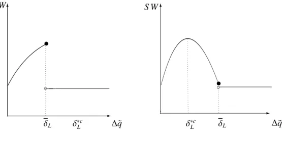
At the discontinuity point∆˜q = δL, we have that S W(δL) > S W.
If∆˜q ≤ δL, then S W is concave down and ∂S W∂∆˜q = 0 is equivalent to ∆˜q∗=
(θ−θ)(θ+θ−2α+2µ) 2β = δ
c∗
L. Two cases
emerge depending on the relative position of δc∗ L and δL.
Case 1: if µ > 3θ−θ−2α2 , then δc∗L > δL. The maximum of S W is achieved at δL.
Case 2: if µ ≤ 3θ−θ−2α2 , then 0 < δc∗
6 - -6 ∆˜q ∆˜q δL δ∗cL δ∗cL δL t t b b S W S W
Figure 4 – The global welfare’s possible curves for low values of the marginal production cost
• If 2θ − θ < α < 2θ − θ, three sub-cases have to be distinguished:
Case a: 2θ − θ < α < MC1.
The global welfare is as follows:
S W= 1 9q(θ − 2θ+ α)(θ + 4θ − 5α + 6µ) + 1 9˜q(2θ − θ − α)(4θ+ θ − 5α + 6µ) − β(∆˜q) 2− 2γ(θ − θ) if ∆˜q ≤ δ I, S W if ∆˜q > δI.
At the discontinuity point∆˜q = δI, we have that S W(δI) > S W.
When∆˜q ≤ δI,∂S W∂˜q = 0 is equivalent to ∆˜q∗=
(2θ−θ−α)(4θ+θ−5α+6µ) 18β = δ
c∗ I .
We can easily check that δc∗
I > 0 when α < MC1. Two cases emerge depending on the relative position of δ c∗ I
and δI.
• If µ ≤ 4θ−5θ6+α then δc∗
I < δI and the maximum of S W is reached at∆˜q = δc∗I .
• If µ > 4θ−5θ6+α then δc∗
I > δI and the maximum of S W is reached at∆˜q = δI.
Case b: MC1< α < MC2.
S W= 1 9q(θ − 2θ+ α)(θ + 4θ − 5α + 6µ) + 1 9˜q(2θ − θ − α)(4θ+ θ − 5α + 6µ) − β(∆˜q) 2− 2γ(θ − θ) if ∆˜q ≤ ˆδ, S W if ∆˜q > ˆδ.
At the discontinuity point∆˜q = ˆδ, we have S W(ˆδ) > S W. If∆˜q ≤ ˆδ, then ∂S W∂∆˜q = 0 is equivalent to ∆˜q∗= δc∗
I . We have that δ c∗
I > 0 thanks to the inequality α < MC2. Two
cases emerge depending on the position of δc∗I relative to ˆδ. We have δc∗
I > ˆδ if and only if µ >
(θ−θ)(θ+θ−2α)
(2θ−θ−α) . Moreover the sign of µ=
(θ−θ)(θ+θ−2α)
(2θ−θ−α) is the same as the sign of
(θ+ θ − 2α).We have θ + θ − 2α ≥ 0 if and only if α ≤ θ+θ2 and as we check that MC1< θ+θ2 < MC2, we conclude
as follows:
• if MC1< α < θ+θ2 then
– if µ ≤ (θ−θ)(θ+θ−2α)
(2θ−θ−α) , we have δ ∗c
I < ˆδ and the maximum of social welfare is reached when ∆˜q = δ ∗c I .
– if µ > (θ−θ)(θ+θ−2α)
(2θ−θ−α) , we have δ ∗c
I > ˆδ and the maximum of social welfare is reached when ∆˜q = ˆδ.
• if θ+θ2 < α < MC2, in this case (θ+ θ − 2α) is negative so we always have δ∗cI > ˆδ and the maximum of
social welfare is reached at∆˜q = ˆδ.
Case c: MC2< α < 2θ − θ.
Appendix C: The National Labels Case
We prove in this appendix the results relative to the national labels case. Some intermediate results are needed to prove Proposition 2. The price stage is identical to the international label case. Lemma 3 calculates the equilibrium at the quality stage of the game. Lemma 4 gives the decisions of governments to open or not their frontiers. An outline of the remaining of the proof of Proposition 2 is then provided along with the detailed proof of the sub-case82θ − θ < α < MC
1.
Lemma 3. When economies are open and for given labeling criteria ˜q1and˜q2such that9 ˜q1≤ ˜q2, depending on
the marginal costα, three cases emerge at the quality stage of the game: • ifα > 2θ − θ, both firms produce q;
• ifα ≤ 2θ − θ, depending on ∆˜q1and∆˜q2, we have the following10:
– if∆˜q2> ∆˜q1> δI, both firms produce q;
– if∆˜q2> δL≥∆˜q1, Firm 1 produces˜q1and Firm 2 produces q;
– if∆˜q2≤δL, Firm 1 produces q and Firm 2 produces˜q2.
• if 2θ − θ < α < 2θ − θ, depending on∆˜q1and∆˜q2, we have the following:
– if∆˜q2> ∆˜q1> δL, both firms produce q;
– if∆˜q2> δI ≥∆˜q1, Firm 1 produces˜q1and Firm 2 produces q;
– if∆˜q2≤δI, Firm 1 produces q and Firm 2 produces˜q2.
Proof of Lemma 3.
When countries decide to open their economies, three cases emerge at the quality stage of the game depending on parameter α. The payoff matrices in each case are given, then the Nash equilibria are derived.
• If α ≥ 2θ − θ, as given in Result 2, only the low quality firm is active at the price stage of the game when firms produce different qualities. The profits of the firms are given in the payoff matrix below :
1\2 q ˜q2
q Π1= 0 Π1= 2(θ − θ)(α − θ)∆˜q2
Π2= 0 Π2 = −β(∆˜q2)2
˜q1 Π1 = −β(∆˜q1)2 Π1= 2(θ − θ)(α − θ)(∆˜q2−∆˜q1) − β(∆˜q1)2
Π2= 2(θ − θ)(α − θ)∆˜q1 Π2 = −β(∆˜q2)2
• If α ≤ 2θ − θ, as given in Result 2, only the high quality firm is active at the price stage of the game when firms produce different qualities. The firms’ profits are given in the payoff matrix below:
1\2 q q˜2
q Π1= 0 Π1= 0
Π2= 0 Π2= 2(θ − θ)(θ − α)∆˜q2−β(∆˜q2)2
˜q1 Π1= 2(θ − θ)(θ − α)∆˜q1−β(∆˜q1)2 Π1= −β(∆˜q1)2
Π2= 0 Π2= 2(θ − θ)(θ − α)(∆˜q2−∆˜q1) − β(∆˜q2)2
Depending on∆˜q1and∆˜q2, four cases emerge:
– if∆˜q2> ∆˜q1> δL, the Nash equilibrium is (q, q);
– if∆˜q2 > δL≥∆˜q1, the Nash equilibrium is ( ˜q1, q). Another Nash equilibrium (q, q) prevails when
∆˜q1= δLand using SA, we select the equilibrium ( ˜q1, q);
– if δL∆˜q2 −∆˜q1
∆˜q2 < ∆˜q2 ≤δL, two Nash equilibria prevail (q, ˜q2) and ( ˜q1, q). Another Nash equilibrium
(q, q) prevails when∆˜q2 = δL. Using SA, we select (q, ˜q2);
– if∆˜q2≤δL∆˜q2 −∆˜q1
∆˜q2 , the Nash equilibrium is (q, ˜q2). Another Nash equilibrium prevails ( ˜q1, q) when
∆˜q2= δL∆˜q2 −∆˜q1
∆˜q2 and using SA, we select (q, ˜q2).
• If 2θ − θ < α < 2θ − θ, as given in Result 2, both firms are active at the price stage of the game when they produce different qualities. The profits of the firms are given in the payoff matrix below:
1\2 q ˜q2
q Π1= 0 Π1=29∆˜q2(2θ − θ − α)2
Π2= 0 Π2=29∆˜q2(2θ − θ − α)2−β(∆˜q2)2
˜q1 Π1= 29∆˜q1(2θ − θ − α)2−β(∆˜q1)2 Π1= 29(∆˜q2−∆˜q1)(2θ − θ − α)2−β(∆˜q1)2
Π2 =29∆˜q1(2θ − θ − α)2 Π2= 92(∆˜q2−∆˜q1)(2θ − θ − α)2−β(∆˜q2)2
– if∆˜q2> ∆˜q1> δI, the Nash equilibrium is (q, q);
– if∆˜q2 > δI ≥∆˜q1, the Nash equilibrium is ( ˜q1, q). Another Nash equilibrium (q, q) prevails when
∆˜q1= δI and using SA, we select ( ˜q1, q);
– if δI∆˜q2∆˜q−∆˜q1
2 −
2
9β(2θ − θ − α) 2 ∆ ˜q1
∆˜q2 < ∆˜q2 ≤δI then two Nash equilibria prevail : (q, ˜q2) and ( ˜q1, q).
Another Nash equilibrium (q, q) prevails when∆˜q2= δI and using SA, we select (q, ˜q2);
– if∆˜q2≤δI∆˜q2 −∆˜q1 ∆˜q2 − 2 9β(2θ − θ − α) 2 ∆ ˜q1
∆˜q2, then(q, ˜q2) is a Nash equilibrium. Another Nash equilibrium
From Lemma 3, at most one firm will be labeled at the quality stage of the game and the active label always satisfies∆˜qi ≤ δL for low marginal costs and∆˜qi ≤ δI for intermediate marginal cost. The equilibrium at the
second stage of the game where countries decide whether to open or close their economies is given in Lemma 4. The proof of Lemma 4 follows the same steps as the proof of Lemma 2 and is omitted here.
Lemma 4. The decision of governments to open (O) or close (O) their economies for given labeling criteria ˜q1
and˜q2such that11 ˜q1 ≤ ˜q2, is as follows:
• ifα ≥ 2θ − θ, both governments are indifferent between open and closed economies. • ifα ≤ 2θ − θ, we have the following:
– if∆˜q2> ∆˜q1> δL, both governments are indifferent between open and closed economies;
– otherwise, both governments choose O and economies are open. • if 2θ − θ < α < 2θ − θ, we have the following:
– if∆˜q2> ∆˜q1> δI, both governments are indifferent between open and closed economies;
– otherwise, the government of the non-labeled firm chooses O. The decision of the government of the labeled firm depends on the marginal costα:
∗ if 2θ − θ < α < MC1, the government of the labeled firm chooses O and economies are open;
∗ if MC1< α < MC2, then if there exist i such that∆˜qi< ˆδ, the government of the labeled firm
chooses O and economies are open. Otherwise, it chooses O and economies are closed; ∗ if MC2 < α < 2θ − θ, the government of the labeled firm chooses (O) and economies are
closed.
The remaining of the Proof of Proposition 2.
We now calculate the labeling criteria ˜q1and ˜q2at the Sub-Game Perfect Nash Equilibrium. The first stage of the
game amounts to determine the Nash equilibria of the labeling stage where each national authority maximizes the social welfare of its own country taking the criteria of the other authority as given.
The three cases about the marginal cost α that emerged at the three last stages of the game naturally emerge here. The proof is quite technical and tedious but we always proceed in the same manner. First, we divide the space (∆˜q1, ∆˜q2) in zones defined by the equilibrium given by Lemmas 3 and 4. In each zone, we determine candidates
to equilibrium. Finally, we examine whether these candidates are equilibria. We present the detailed proof only in the case 2θ − θ < α < MC1. The proofs of all other cases follow the same reasoning and can be provided on
request.
The case 2θ − θ < α < MC1
social welfare of the country of the labeled firm is given by the government’s surplus T SLO(which is the sum of
consumers’ surplus and the labeled firm’s profit) minus the environmental damage.
S WL= TSLO− 2θ − θ − α 3 (γ − µ ˜q) − θ − 2θ + α 3 (γ − µq), which equals S WL= q 18(−5θ 2 − 2θ2− 5α2+ 2θθ + 8αθ + 2αθ) + ˜q 18(14θ 2 − 7θ2+ 5α2− 2θθ − 26αθ+ 16αθ) −β(˜q − q)2− (θ − θ)γ+1 3µ(2θ − θ − α)˜q + 1 3µ(θ − 2θ + α)q. The social welfare of the country of the non-labeled firm is given by the government’s surplus T SNLO(which is
the sum of consumers’ surplus and the non-labeled firm’s profit) minus the environmental damage.
S WNL= TSNLO− 2θ − θ − α 3 (γ − µ ˜q) − θ − 2θ + α 3 (γ − µq), which equals S WNL= q 18(7θ 2 − 14θ2− 5α2+ 2θθ − 16αθ + 26αθ) + ˜q 18(2θ 2 + 5θ2+ 5α2− 2θθ − 2αθ − 8αθ) − (θ − θ)γ+1 3µ(2θ − θ − α)˜q + 1 3µ(θ − 2θ + α)q. We notice that S WLis a quadratic function (concave down) of ˜q and that S WNLis an increasing linear function
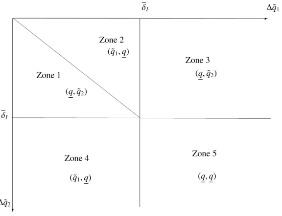
of ˜q. Figure 5 defines the equilibria that prevail at the quality stage of the game in this case.
Zone 1 is characterized by∆˜q1 ≤ ∆˜q2and∆˜q2 ≤δI. Let us find the candidates for Nash equilibria in this
zone. Countries’ social welfare are given by: S W1 = S WNL( ˜q2) and S W2 = S WL( ˜q2). The social welfare of the
country of the labeled firm S W2is maximized at∆˜q2∗= ˆ δ 2 + 1 6βµ(2θ − θ − α) = δ ∗d I .
We have that δ∗dI ≤δIis equivalent to µ ≤ µ2. Thus we distinguish two cases12:
• Case 1: if µ ≤ µ2, the first candidate to equilibrium in zone 1 is given by the pair (∆˜q2= δ∗dI , ∆˜q1≤δ∗dI ).
• Case 2: if µ > µ2, the second candidate to equilibrium in zone 1 is given by the pair (∆˜q2= δI, ∆˜q1≤δI).
? -δI δI ∆˜q1 ∆˜q2 Zone 1 Zone 2 Zone 3 Zone 4 Zone 5 ( ˜q1, q) (q, ˜q2) ( ˜q1, q) (q, ˜q2) (q, q)
Figure 5 – Equilibria at the quality stage of the game for 2θ − θ < α < MC1.
Case 1:µ ≤ µ2. For a fixed∆˜q2= δ∗dI ,
S W1( ˜q1, ˜q2= δI∗d+ q) = S WNL(δ∗dI + q) if ∆˜q1≤δ∗dI , S WL( ˜q1) if δ∗dI < ∆˜q1≤δI, S WNL(δ∗dI + q) if ∆˜q1> δI. (1)
We notice that S W1( ˜q1, ˜q2 = δI∗d+ q) is constant on [q, δ∗dI + q], decreasing and concave down on (δ∗dI +
q, δI+ q], and constant again if ˜q1> δI+ q. To find the maximum of S W1, we need to compare S WNL(δ∗dI + q) and
S WL(δ∗dI + q). We have that S WL(δ∗dI + q) ≥ S WNL(δ∗dI + q) if and only if µ < µ1. We easily check that µ1 < µ2.
Thus13,
• If µ < µ1, S WL(δ∗dI + q) > S WNL(δ∗dI + q) and the first candidate to equilibrium is not an equilibrium as
there is a profitable deviation for Authority of Country 1.
• If µ1< µ < µ2, S WL(δ∗dI +q) < S WNL(δ∗dI +q) and there is no profitable deviation for Authority of country
1 . We need now to check the possible deviations of Authority of Country 2.
Let us check the possible deviations of Authority of Country 2 when µ1< µ < µ2and for a fixed∆˜q∗1≤δ ∗d I .
S W2( ˜q1∗, ˜q2)= S WNL( ˜q∗1) if ∆˜q2< ∆˜q∗1, S WL( ˜q2) if ∆˜q∗1≤∆˜q2≤δI, S WNL( ˜q∗1) if δI < ∆˜q2. (2)
We notice that S W2( ˜q1∗, ˜q2) is constant on [q, ˜q∗1), increasing then decreasing on [ ˜q∗1, δI + q] with the
max-imum reached at δ∗d
I + q and constant again if ˜q2 > δI + q. To find the maximum of S W2( ˜q1∗, ˜q2), we need to
compare S WNL( ˜q∗1) and S WL(δ∗dI + q). We have that S WL(δ∗dI + q) > S WNL( ˜q∗1) if and only if∆ ˜q∗1≤ H. We check
that14H< δ∗dI . The equilibrium is then given by the pair (∆˜q1∗≤ H, ∆˜q∗2= δ∗dI ).