HAL Id: halshs-01662808
https://halshs.archives-ouvertes.fr/halshs-01662808
Preprint submitted on 13 Dec 2017
HAL is a multi-disciplinary open access
archive for the deposit and dissemination of
sci-entific research documents, whether they are
pub-lished or not. The documents may come from
teaching and research institutions in France or
L’archive ouverte pluridisciplinaire HAL, est
destinée au dépôt et à la diffusion de documents
scientifiques de niveau recherche, publiés ou non,
émanant des établissements d’enseignement et de
recherche français ou étrangers, des laboratoires
Missing Poor and Income Mobility
Mathieu Lefebvre, Pierre Pestieau, Grégory Ponthière
To cite this version:
Mathieu Lefebvre, Pierre Pestieau, Grégory Ponthière. Missing Poor and Income Mobility. 2017.
�halshs-01662808�
WORKING PAPER N° 2017 – 56
Missing Poor and Income Mobility
Mathieu Lefebvre
Pierre Pestieau
Gregory Ponthière
JEL Codes: I32
Keywords: poverty, measurement, mortality, missing poor, income mobility
P
ARIS
-
JOURDAN
S
CIENCES
E
CONOMIQUES
48, BD JOURDAN – E.N.S. – 75014 PARIS TÉL. : 33(0) 1 80 52 16 00=
www.pse.ens.fr
CENTRE NATIONAL DE LA RECHERCHE SCIENTIFIQUE – ECOLE DES HAUTES ETUDES EN SCIENCES SOCIALES – E
Missing Poor and Income Mobility
Mathieu Lefebvre
yPierre Pestieau
zGregory Ponthiere
xDecember 5, 2017
Abstract
Higher mortality among the poor leads to selection biases in poverty measures. Whereas existing attempts to deal with the "missing poor" problem assume the absence of income mobility and assign to the prema-turely dead a …ctitious income equal to the last income enjoyed, this paper relaxes that assumption in order to study the impact of income mobility on the size of the missing poor bias. We use data on poverty above age 60 in 12 countries from the EU-SILC database, and we compare standard poverty rates with the hypothetical poverty rates that would have pre-vailed if (i) all individuals, whatever their income, had enjoyed the same survival conditions (the ones of the highest income class), and if (ii) all individuals within the same income class had been subject to the same income mobility process. It is shown that taking income mobility into ac-count has adverse e¤ects on corrected poverty measures across ac-countries, and that it a¤ects international comparisons in terms of old-age poverty. Keywords: poverty, measurement, mortality, missing poor, income mo-bility.
JEL classi…cation code: I32.
The authors would like to thank Yves Arrighi, Thomas Baudin, Xavier Chojnicki, David Crainich, Fabrice Etilé, Hubert Jayet, Jean-François Laslier, Claudia Senik, Stephane Vigeant, as well as participants of seminars at LEM (Lille), PSE (Paris) and IRES (Université catholique de Louvain).
yBETA, University of Strasbourg.
zUniversity of Liège, CORE and Paris School of Economics.
xUniversity Paris East (ERUDITE), Paris School of Economics and Institut universitaire de France. [corresponding author]. Address: Paris School of Economics, 48 boulevard Jour-dan, O¢ ce R 3.66, 75014 Paris, France. E-mail: [email protected]. Telephone 0033-0180521919.
1
Introduction
Despite the rise of the modern Welfare State, our economies can be regarded, at the beginning of the 21st century, as Malthusian economies, in the sense that poor individuals still face nowadays higher mortality rates than non-poor per-sons, in line with the "positive population check" phenomenon underlined by Malthus (1798). Although the extent of overmortality of the poor has been re-duced since Malthus’s epoch, empirical studies show that there exists nowadays an increasing non linear relationship between income and life expectancy.1
As this was stressed by Kanbur and Mukherjee (2007), the positive corre-lation between income and life expectancy leads to selection biases in standard poverty measures. The intuition behind this measurement problem is simple: poor persons face higher mortality rates than non-poor persons, which implies that, when measuring poverty at the old age, one concentrates on the surviv-ing populations only, in which the poor are necessarily under-represented with respect to the non poor. This phenomenon can be coined the "missing poor" phenomenon, in line with Sen’s (1998) "missing women" problem.
In order to correct for the missing poor problem, Kanbur and Mukherjee (2007) proposed to assign, to the prematurely dead poor persons, a …ctitious income, and to compute hypothetical poverty rates under the hypothetical in-come distribution. Alternatively, Lefebvre et al (2013) proposed to assign to all prematurely dead persons (poor and non poor) a …ctitious income, and to compute poverty rates on that new hypothetical income distribution.
Under those two approaches, the …ctitious income assigned to the prema-turely dead consists of the last income that the individual enjoyed before dying. This assignment procedure constitutes a good proxy in an economy where there is little or no income mobility. However, in economies with stronger income mobility, taking the last income as a proxy of the income level that would have been enjoyed in case of survival constitutes a stronger assumption.
The goal of this paper is precisely to reexamine the missing poor problem for poverty measurement while taking income mobility into account. For that pur-pose, we propose to compare standard old-age poverty measures with corrected old-age poverty measures that assign to prematurely dead individuals not the last income enjoyed before dying, but the income that would have been enjoyed in case of survival given the prevailing income mobility process.
Our motivation for studying the e¤ect of income mobility on the missing poor problem goes as follows. Actually, if there is a strong upward (resp. downward) income mobility conditional on survival, assigning to the prematurely dead a …ctitious income equal to the last income enjoyed could lead to overestimate (resp. underestimate) the size of the selection bias due to income-di¤erentiated mortality. To illustrate that point, consider an economy with two ages of life - young and old -, with three income levels - low, middle and high - and with probabilities to survive to the old age, equal respectively to s, s and ^s (with
1On this relation, see Duleep (1986), Deaton and Paxson (1998), Backlund et al (1999), Deaton (2003), Jusot (2003), Duggan et al (2007), and Salm (2007).
s < s < ^s). For simplicity, let us assume that there is an equal number of young persons in each income group, and that only low income persons are poor. Let us consider three income mobility processes, given by matrices A, B and C.
A = 0 @ 10 01 00 0 0 1 1 A ; B = 0 @ 00 00 11 0 0 1 1 A ; C = 0 @ 11 00 00 1 0 0 1 A
Table 1 compares the standard poverty rates at the old age (column I) with the hypothetical poverty rates that would prevail if all individuals enjoyed the survival rate of the rich (i.e. ^s), while assigning to missing persons …ctitious incomes equal either to the last income enjoyed (column II) or to the income that they would have enjoyed in case of survival given the income mobility process (column III). The last two columns show the associated selection bias, measured by the gap between the corrected and the standard poverty rates, the former being computed either by assigning the last income as a …ctitious income (column IV) or by assigning as …ctitious income the income that would have been enjoyed in case of survival (column V).2
old-age poverty rate selection bias
(I) (II) (III) (IV) = (II)-(I) (V) = (III)-(I) (standard) (hypothetical) (hypothetical)
s = ^sfor all s = ^sfor all last income income mobility
A s+s+^s s<13 13 31 13 s+s+^s s 13 s+s+^s s
B 0 13 1 s^s 0 13 1 s^s > 0 0
C 1 23+13ss^< 1 1 13 ss^ 1 < 0 0
Table 1: Income mobility and selection bias in a simpli…ed economy. In the absence of income mobility (matrix A), the gap between corrected and standard poverty rates does not depend on whether the assigned …ctitious income is the last enjoyed or is the one that would have been enjoyed in case of survival. However, under strong upward income mobility (matrix B), assigning a …ctitious income equal to the last income enjoyed leads to overestimate the number of missing poor. Indeed, all prematurely dead persons would, in case of survival, have here escaped from poverty, so that counting some missing persons as poor leads to overestimate the selection bias due to income-di¤erentiated mortality. On the contrary, under strong downward income mobility (matrix C), using the last income enjoyed as a …ctitious income leads to underestimate the bias. Abstracting from income mobility leads here to ignore that middle-income young individuals who died prematurely would have fallen into poverty in case of survival, implying an underestimation of the selection bias.
In order to examine the impact of income mobility on the missing poor problem, this paper uses data on poverty above age 60 in 12 countries from the
2Note that, in cases B and C, income-di¤erentiated mortality leads to no bias, since the proportion of poor persons at the old age is independent from the gap in survival rates between the poor and the non poor.
EU-SILC database.3 We …rst compare standard old-age poverty rates with the hypothetical old-age poverty rates that would have prevailed if (i) all individuals, whatever their income, had enjoyed the same survival conditions (the ones of the highest income class), and if (ii) all individuals within the same income class had been subject to the same income mobility process. Assumption (ii) amounts to assign to prematurely dead persons a …ctitious income equal to the one that would have been enjoyed in case of survival, given the income mobility process (conditional on survival). This procedure requires us to estimate actual income mobility processes in the economies under study. Then, in order to assess the impact of income mobility, we compare the corrected poverty rates under income mobility with the ones obtained under no income mobility for missing persons. Anticipating on our results, we show that there exist sizeable gaps between standard old-age poverty rates and poverty rates corrected under assumptions (i) and (ii), and that those gaps a¤ect the comparison of old-age poverty across countries and gender. When comparing those gaps with the ones obtained while assuming no income mobility (and thus relaxing assumption (ii)), we show that upward income mobility reduces those gaps, but to an extent that varies signif-icantly across countries. Thus taking income mobility into account matters for the measurement of the selection bias induced by income-di¤erentiated mortal-ity. In addition, our analysis shows that the size of the gap between the standard and corrected poverty rates depends also on whether the poverty line is based either on the pre-adjustment income distribution, or on the post-adjustment income distribution, and on whether the poverty line is relative or absolute.
Our paper is related to the literature on the "missing poor", such as Kanbur and Mukherjee (2007) and Lefebvre et al (2013, 2017). Our paper, which ex-amines poverty measurement in presence of income-di¤erentiated mortality, is also related to the growing literature on lifetime poverty, such as Foster (2009), Bossert et al (2011) and Hoy and Zheng (2011), since the assignment of …ctitious incomes to the prematurely dead constitutes a solution to allow for the com-parison of poverty along lives of unequal lengths. Finally, we also complement the literature on income mobility (Fields and Ok, 1996, 1999; Van Kerm, 2004, 2009; Alperin and Van Kerm, 2010; Van Kerm and Alperin, 2013), by examining the relation between income mobility and the missing poor problem.4
The paper is organized as follows. Section 2 develops a simple model of old-age poverty measurement under income-di¤erentiated mortality. Section 3 compares standard and hypothetical old-age poverty rates for 12 European countries. Section 4 studies the robustness of the correction of poverty rates to the assumption on income mobility. Section 5 examines the robustness of our results to allowing the poverty line to vary with the addition of missing persons. Finally, Section 6 assesses the robustness of our results to adopting an absolute poverty line equal to 10 euros a day. Section 7 concludes.
3The countries are Bulgaria, Czech Republic, Denmark, Estonia, Finland, Hungary, Italy, Norway, Poland, Portugal, Romania and Sweden.
2
Missing poor: theory
2.1
The framework
Let us consider a cohort of size N 2 N. Each member of that cohort lives the young age for sure, and reaches the old age with a probability s. There exists K income levels y1; :::; yK 2 R+, including a particular poverty line yP. Those
income levels are ranked in increasing order:
y1< ::: < yP < ::: < yK (1)
The distribution of income at the young age is represented by a vector n of size K, whose entries n1; :::; nK are the number of young individuals with
incomes y1; :::; yK.
To each income level yk enjoyed at the young age is associated a survival
probability to the old age denoted by sk 2 Q+. We assume that there exists a
perfect rank correlation between income and survival conditions:
s1< ::: < sP < ::: < sK (2)
Conditionally on survival to the old age, each member of the cohort enjoys a particular income level at the old age. The income mobility process conditionally on survival to the old age is described by the right-stochastic matrix :
0
@ :::11 :::::: :::1K
K1 ::: KK
1
A (3)
where ik2 Q+is the probability that a young individual with income yienjoys,
in case of survival to the old age, an income yk.
The distribution of income at the old age is represented by a vector m of size K, whose entries m1; :::; mK are the number of young individuals with incomes
y1; :::; yK. The distribution of income at the old age can be obtained from the
income distribution at the young age as follows:
m= 0n (4)
where the matrix is the Hadamard product of matrices and : 0 @ :::11 :::::: :::1K K1 ::: KK 1 A | {z } 0 @ s:::1 :::::: s:::1 sK ::: sK 1 A | {z } = 0 @ 11:::s1 :::::: 1K:::s1 K1sK ::: KKsK 1 A (5)
2.2
Measuring old-age poverty
For a given poverty line yP, the standard poverty rate at the old age is:
P = PX1 i=1 mi K X j=1 mj = PX1 i=1 K X l=1 nlsl li K X j=1 K X l=1 nlsl lj (6)
The level of the old-age poverty rate depends on three forces: …rst, the income distribution at the young age; second, the income mobility process; third, the survival conditions, which are di¤erentiated according to the income level.5 Whereas the in‡uence of the income distribution at the young age and of the income mobility process are something worth being captured by old-age poverty measures, it is not clear to see to what extent one may want the old-age poverty rate to be dependent on income-di¤erentiated survival conditions.
Actually, as shown in Lefebvre et al (2017), there is only one case where the old-age poverty measure is independent from income-di¤erentiated survival conditions, which is when all young individuals face the same expected extent of poverty, whatever their initial income is:
PX1 j=1 ij = PX1 j=1 kj8i 6= k (7)
That condition is unlikely to be satis…ed by actual income mobility processes. Hence, the fact that poor persons face worse survival conditions is likely to a¤ect the level of poverty measures at the old age.
2.3
Selection bias
Standard poverty measures P su¤er from a selection bias, which is due to the fact that poor persons are under-represented in the old-age population, because of worse survival conditions. In order to measure that bias, let us …rst de…ne the corrected poverty measure P as the poverty measure based on a hypothetical population where all income classes would face similar survival conditions, for instance the ones of the highest income class:
P = PX1 i=1 mi K X j=1 mj (8)
5Note that, if survival rates were equal for all income groups, then it would be possible to factorize by s at the numerator and at the denominator of P , so that the old-age poverty rate would be completely independent from survival conditions.
where each income class has faced the same survival conditions, that is: mi= K X l=1 nlsK li8i (9)
Note that, whatever one takes the survival probability of the highest income class sK or any other survival probability si, this has no in‡uence on the
cal-culation of the corrected poverty rate P , since the uniform survival probability multiplies all terms at the numerator and at the denominator of P .
The poverty rate P is not observed; this requires to compute the hypothetical old-age poverty rate that would have prevailed if all income classes were facing the same survival conditions, so that no selection bias would arise.
In absolute terms, the selection bias B can be calculated as the di¤erential between the corrected poverty measure P (where all income groups would face similar survival conditions) and the standard poverty measure P :
B P P = PX1 i=1 K X l=1 nlsK li K X j=1 K X l=1 nlsK lj PX1 i=1 K X l=1 nlsl li K X j=1 K X l=1 nlsl lj (10)
In relative terms, the selection bias b can be computed as:
b P P
P (11)
In order to have an exact measure of the (absolute and relative) selection bias induced by income-di¤erentiated mortality, one should have a perfect knowledge of income-di¤erentiated survival conditions, as well as a perfect knowledge of the pure income mobility process (i.e. conditional on survival).
This piece of information is not directly available. But using distinct data-bases, we can obtain estimates of income-speci…c survival probabilities ^si and
estimates of probabilities of income mobility ^ij, which can be used to provide a
proxy measure of the selection bias at work in old-age poverty measures. Hence, conditionally on an observed income distribution at the young age, the selection bias can be approximated by:
^ B P^ P = PX1 i=1 K X l=1 nl^sK^li K X j=1 K X l=1 nl^sK^lj PX1 i=1 K X l=1 nls^l^li K X j=1 K X l=1 nls^l^lj (12)
while the relative selection bias ^b can be approximated by: ^b P^ P
^
When the survival conditions are similar for all income classes, that is, when ^
si ^sj for all i; j, then the (absolute or relative) selection bias is small, since
in that case the corrected and the standard poverty rates are close. On the contrary, when there is a large di¤erential between the survival conditions faced by di¤erent income classes, the measured selection bias is likely to be larger.
The size of the measured selection bias depends also on the prevailing income mobility process. When the income mobility process involves strong upward mobility, so that most surviving individuals tend to escape from poverty, then both the numerators of the …rst and the second term are close to zero, implying a low size of the measured selection bias in absolute terms (but not necessarily in relative terms). On the contrary, if the income mobility process involves no mobility or downward mobility, the di¤erential in survival conditions is likely to lead to higher levels for the measured (absolute or relative) selection bias.
Given the central impact of the income mobility process on the size of the measured selection bias, it is important, when considering the "missing poor" phenomenon, to estimate income mobility processes, in order to quantify the extent to which income-di¤erentiated mortality leads to selection biases in old-age poverty measures. This is the task of the next section.
3
Missing poor: empirics
3.1
The data
The analysis is based on the EU-SILC (cross-sectional and longitudinal) data-bases for the years 2006 to 2012, and on life expectancy tables by level of education from EUROSTAT. Our sample focuses on people aged 60 and more, and involves 12 countries: Bulgaria (N = 5064), Czech Republic (N = 6307), Denmark (N = 1449), Estonia (N = 3671), Finland (N = 6830), Hungary (N = 6797), Italy (N = 13934), Norway (N = 3077), Poland (N = 9044), Portugal (N = 5155), Romania (N = 5951) and Sweden (N = 4158).6
We take as a baseline the poverty rates at age 60 + in 2012 in those 12 coun-tries, as calculated from the cross-sectional EU-SILC database. We then calcu-late, for those 2012 poverty rates, the selection bias due to income-di¤erentiated mortality. As mentioned above, the measurement of the selection bias in old-age poverty measures requires to have estimates of how survival conditions vary with the income level, as well as estimates of the income mobility process at work (conditionally on survival). The next two subsections describe how those estimates can be obtained for the countries in our sample.
3.1.1 Life expectancy by income class
To our knowledge, there exists no database with lifetables by income levels for European countries. However, EUROSTAT provides, for a number of European countries, lifetables by education levels (see Table 2).
Life expectancy at age 60
Men Women
Countries Primary Secundary Tertiary Primary Secundary Tertiary Bulgaria 14.9 18.4 19.9 20.6 22.6 23.4 Czech R. 14.5 19.5 20.3 23.0 23.7 23.8 Denmark 20.5 21.5 22.8 23.8 24.9 25.5 Estonia 14.3 19.0 20.6 22.1 24.3 25.7 Finland 21.1 21.8 23.1 25.6 26.2 26.9 Hungary 14.2 18.9 20.1 21.1 23.2 23.4 Italy 22.2 24.5 24.5 26.7 27.8 27.8 Norway 21.3 22.7 23.7 24.5 25.9 26.7 Poland 17.4 18.6 21.6 23.5 23.9 25.3 Portugal 21.3 23.2 23.9 25.9 26.3 27.4 Romania 16.2 19.2 19.1 21.8 23.0 23.2 Sweden 22.0 23.0 23.9 24.6 26.0 26.4
Table 2: Life expectancy at age 60 by education level, 2012. Source: EUROSTAT.
From these numbers, it is possible to estimate lifetables by income class using a weighted ordinary least square regression, as in Bossuyt et al (2004) and Van Oyen et al (2005). For that purpose, we take advantage of the high correlation that exists between education and income and their similar impact on health to extrapolate mortality by income class on the basis of the mortality by education. Our methodology is presented in details in the Appendix.
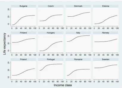
Figures 1 and 2 present estimates of life expectancy at age 60 by income class in each country for the year 2012, for, respectively, men and women.
The slope of the income/life expectancy gradient is usually steeper for males than for females. Note also that there exists a strong heterogeneity within our sample. Whereas the di¤erential between life expectancies by income classes re-mains relatively low for Nordic countries, it is signi…cantly larger among Eastern European countries.
Life expectancy statistics by income classes allow us to quantify, for each country and for each gender, the missing persons, that is, those who died pre-maturely in comparison to individuals enjoying the best survival conditions (i.e. the highest income class). Actually, in a two period model, the ratio of the survival probability to the old age within a high income class to the survival probability to the old age within a low income class can be approximated by the ratio of the two associated life expectancies. Hence, it is possible to adjust the size of each income class for each country and each gender by multiplying its initial size by an adjustment factor equal to the ratio of the life expectancy in the top income class to the life expectancy within the income class under study. For the sake of illustration, Table 3 shows the associated adjustment factors for the particular case of the bottom income class.
Figure 1: Life expectancy by income class at age 60, men, 2012.
Figure 2: Life expectancy by income class at age 60, women, 2012.
Life expectancy at age 60 Adjustment factor Bottom income class Top income class
Countries Males Females Males Females Males Females Bulgaria 13,5 19,0 22,3 24,5 1,65 1,29 Czech R. 15,0 22,0 24,0 25,1 1,60 1,14 Denmark 20,2 23,5 22,8 25,8 1,13 1,10 Estonia 14,5 22,9 20,3 25,6 1,41 1,12 Finland 20,2 25,3 23,3 26,8 1,15 1,06 Hungary 15,0 20,9 21,2 23,9 1,41 1,14 Italy 21,3 25,9 24,6 27,5 1,16 1,06 Norway 21,0 24,2 23,2 26,2 1,11 1,08 Poland 16,4 22,9 20,7 25,0 1,26 1,09 Portugal 20,0 25,2 23,2 26,6 1,16 1,06 Romania 16,2 21,2 20,0 23,0 1,24 1,09 Sweden 21,5 24,6 23,6 26,5 1,10 1,07
Table 3: Life expectancy at age 60 for the bottom and top income classes, with the associated adjustment factors.
Adjustment factors are larger for males than for females. These tend to be quite small for Nordic countries, and larger for Eastern European countries. In the light of this, we expect that selection biases due to income-di¤erentiated mortality di¤er signi…cantly across countries.
3.1.2 Income mobility matrices
In order to obtain income mobility matrices, we use data from Longitudinal EU-SILC. This database contains less information than in the cross-sectional database but covers, for each individual, the last four years. These data allow us to follow the same individual across time. The sample used to estimate income mobility for our reference year of 2012 is based on the EU-SILC Longitudinal databases between 2009 and 2012. In each longitudinal database the sample is based on four subgroups of equal size and each one representing the total population of each year. Each year, the subgroup that completes four years is dropped from the sample and replaced by another equivalent, meaning that each individual or family can only be followed by a period of four years. For example, the 2012 longitudinal database includes individuals who were followed between 2009 and 2012, between 2010 and 2012 and between 2011 and 2012. So there is an overlap between the various longitudinal databases.7
We exploit four longitudinal data sets, covering the periods 2006-2007-2008-2009, 2007-2008-2009-2010, . . . , 2009-2010-2011-2012. Income mobility is ob-tained by comparing pairs of income for a given individual in periods t and t 1. As for poverty measurement, we rely on individual single-adult equival-ized household disposable income (according to the modi…ed-OECD equivalence
7The coverage is not uniform across countries: some years are not available in some coun-tries.
scale). Following Alperin and Van Kerm (2013), we only keep individuals with income larger than zero in two consecutive years, respectively.8 The individual income in each year refers to equivalent income at 2012 constant prices (us-ing the harmonized index of consumer prices, available from EUROSTAT) such that all income changes are in real terms. All results were calculated using the longitudinal weights available.
We are interested in mobility as a positional change in the income distribu-tion. More speci…cally, we want to evaluate the probability that an individual in an income category yi goes one year later in a category yj. Given our
pur-pose, we are interested in absolute income mobility and not relative one such as mobility across deciles (in the sense of Fields and Ok, 1999). We can then look at mobility across income class as the ones we use in our poverty measure.
To maximize sample size, income mobility is calculated based on annual income transitions following the aggregation of all annual transitions in the suc-cessive waves of EU-SILC. This allows to obtain a higher number of observations but also to get rid of some speci…c shock that could happen in one year. How-ever, 100 income classes may be too many to obtain a complete mobility matrices when looking at the old age. We can look at mobility across, for instance, 10 income groups.9
The computed income mobility matrices are presented by country and gender in the Appendix. Those matrices show that there exists a signi…cant downward and upward income mobility, especially around the diagonal of the matrices, that is, towards income classes that are close to the initial income class to which the person belongs. In the light of this, the correction of poverty rates for mortality di¤erentials could hardly ignore income mobility, since, given this mobility, it is not certain that a person who died prematurely would, in case of survival, have enjoyed the same income level as the one enjoyed when being still alive.
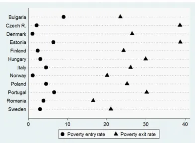
Since we are mainly interested in whether those surviving are much into poverty or not, a most crucial piece of information consists in the tendency of individuals to move in or out of poverty. To summarize the information contained in income mobility matrices, Figure 3 displays, for each country, the probability to exit poverty and the probability to enter poverty for the people aged 60 and more. A person is here considered as poor if her income is below a poverty line set at 60 percent of her country’s median income.10 Figure 3
presents for each year of a longitudinal dataset the poverty exit rates (i.e. the fraction of individuals in poverty at time t 1 that are not poor at time t) and the poverty entry rates (i.e. the fraction of individuals not in poverty at time t 1 that are poor at time t). There are important di¤erences among countries both in terms of entry and exit rates.
8Extreme values of income, which were identi…ed using the cross-section databases, were eliminated, in line with Alperin and Van Kerm (2013).
9For instance, in the case of Sweden, we consider classes of 5000 euros. This implies, given that the poverty line is …xed at 14988 euros, that only those in the three …rst groups are poor in t 1:
1 0The median income is computed on the basis of the initial, actual income distribution, that is, before the adjustment of missing persons is made. See the Appendix for the poverty thresholds.
Figure 3: Poverty entry and exit rate for the year 2012-people aged 60+.
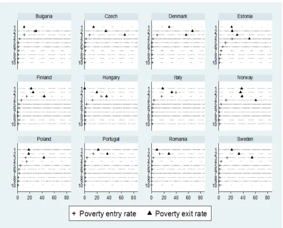
We can also calculate, for each income class, the probability to enter or exit poverty.11 Figure 4 shows that the probability to enter poverty tends generally
to be smaller for people who belong initially to higher income classes. Hence, the property of equal probability to enter poverty discussed in Lefebvre et al (2017) is clearly not satis…ed, implying that income-di¤erentiated mortality will interfere with the measurement of poverty.
The probability to exit poverty is generally lower for those who belong to lower income classes. Those probabilities to exit poverty di¤er signi…cantly from zero, which suggests that, among the poor who died prematurely, some could have, in case of survival, escaped from poverty. Thus taking income mobility into account matters for the de…nition of appropriate counterfactuals.
Despite those general tendencies, there are important di¤erences among countries in terms of entry and exit. In Estonia and Poland, we observe entry into poverty for higher income classes, while in Sweden and Denmark, poverty dynamics is limited across the poverty line.
1 1Obviously, the exit rate is only available for lower income classes; i.e those which are below the poverty line, and the poverty entry rate is not available for lower income classes.
Figure 4: Poverty entry rates and exit rates for year 2012, by income class (people aged 60 and more).
3.2
Results
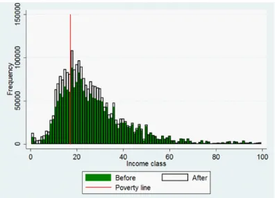
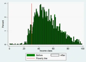
On the basis of income-speci…c life expectancies computed in Section 3.1.1, we calculate, for the 12 countries under study, the number of missing persons in each initial income class (taken from the cross-sectional EU-SILC database for year 2012), to which we assign a …ctitious income using transition matrices estimated in Section 3.1.2. As an illustration, Figure 5 shows, for Bulgaria, the income distribution (in frequency), before and after the addition of missing persons, i.e. those who died but would have survived if they had bene…ted from the survival conditions of the highest income class.12
Figure 5: Income distribution (frequency) in Bulgaria (men and women aged 60+), 2012, before and after the addition of
missing persons.
Figure 6: Income distribution (density) in Bulgaria (men and women aged 60+), 2012, before and after the addition
of missing persons.
On the basis of frequencies, it is possible to derive the distribution in density (Figure 6), which allows us to visualize directly the impact of the addition of missing persons on the measurement of poverty. The di¤erence between the two
income distributions re‡ects not only the addition of prematurely dead persons, but, also, the postulated counterfactual (the …ctitious income of each added missing person being determined by the prevailing income mobility process).
Assuming a constant poverty line, the variation in the poverty headcount measure can be computed directly from the density graph, by calculating the extra percent of individuals who lie on the left of the poverty line. In the case of Bulgaria, the number of added poor persons is substantial, and exceeds 2 percents of the population. This implies that, in the case of Bulgaria, if all individuals, whatever their income levels are, had faced the survival conditions of the highest income class, then the poverty rate above age 60 would have increased by about 2 percentage points. One can, on the basis of those calcula-tions, consider that the selection bias induced by income di¤erentiated mortality equals about 2 percentage points in the case of Bulgaria.
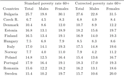
Using the same method, we can compare standard old-age poverty rates with corrected ones by country and gender. Our results are collected in Table 4.13
Standard poverty rate 60+ Corrected poverty rate 60+ Countries Total Males Females Total Males Females
Bulgaria 25.7 19.8 30.1 27.6 22.8 31.5 Czech R. 6.7 4.5 8.3 6.8 4.9 8.4 Denmark 10.4 8.6 12.0 10.7 8.9 12.2 Estonia 16.8 13.1 18.9 18.2 15.6 19.7 Finland 16.5 13.4 19.1 16.9 14.0 19.3 Hungary 7.5 6.8 7.9 8.5 8.3 8.6 Italy 17.0 14.1 19.3 17.5 14.8 19.6 Norway 7.7 4.0 11.0 7.9 4.2 11.2 Poland 14.8 12.5 16.4 15.4 13.6 16.7 Portugal 17.9 16.4 19.1 18.3 17.0 19.3 Romania 15.6 12.2 18.2 16.2 13.1 18.6 Sweden 15.4 10.2 19.7 15.7 10.6 20.0
Table 4: Standard and corrected poverty rates at age 60 + (%), 2012.
For all countries and genders, corrected poverty rates exceed standard poverty rates. This result reveals the existence of some selection biases: in the hypotheti-cal case where all individuals would have faced the same survival conditions, and would have been subject to the same income mobility matrix, old-age poverty measures would have taken levels that are superior to the standard ones. Thus income-di¤erentiated mortality has tended to reduce, by selection, the measured poverty at the old age.
Note, however, that the size of the correction varies across countries and gender. Hence, correcting selection bias may a¤ect the ranking of countries in terms of old-age poverty. For instance, whereas Norway presents a higher poverty rate at age 60+ than Hungary (7.7 % for Norway against 7.5 % for
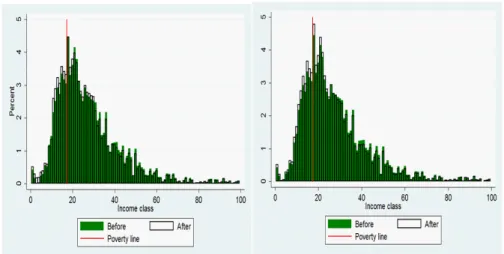
Hungary), this is no longer the case once poverty rates are corrected. Actually, the corrected old-age poverty rate equals 8.5 % in Hungary, against 7.9 % in Norway. This inversion in the international ranking in terms of poverty is illus-trated on Figures 7 and 8, which show the changes in the income distributions in, respectively, Hungary and Norway.
Figure 7: Income distribution (density) in Hungary (men and women aged 60+), 2012, before and after
the addition of missing persons.
Figure 8: Income distribution (density) in Norway (men and women aged 60+), 2012, before and after
The correction also a¤ects the comparison of poverty measures across gender. To illustrate this, take the case of Portugal. The usual poverty rates at age 60 + show that poverty is higher among females than among males (19.1 % for females against 16.4 % for males). There is a 2.7 points di¤erence between female and male’s poverty rates. But in corrected terms, that is, once selection biases are neutralized, the gender gap falls to 19.3 - 17.0 = 1.7 points.
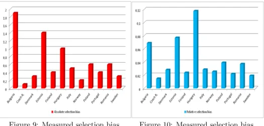
Figure 9, which compares the levels of absolute selection bias across coun-tries, illustrates that the addition of prematurely dead persons has quite adverse e¤ects on the measured old-age poverty across Europe. One part of the di¤eren-tials in the size of selection biases comes merely from the overall level of old-age poverty in uncorrected terms. Clearly, countries with high uncorrected levels of old-age poverty, such as Bulgaria, have higher corrections of poverty rates. This motivates us to look at the levels of relative selection biases (Figure 10).14 In
relative terms, the largest selection biases concern Bulgaria, Estonia and Hun-gary. For those countries, income-di¤erentiated mortality tends to lead to a signi…cant downward bias in the measurement of poverty.
Figure 9: Measured selection bias, absolute terms, 2012.
Figure 10: Measured selection bias, relative terms, 2012.
4
The e¤ect of income mobility
To identify the in‡uence of the income mobility process on the size of measured selection biases, let us now construct another counterfactual than the one con-sidered so far. Instead of assigning to each missing person a …ctitious income equal to the one he would have enjoyed in case of survival given the prevailing income mobility process, let us now assign as a …ctitious income the last income
1 4Relative selection biases are computed by dividing the absolute selection bias by the corrected poverty rate.
enjoyed when being alive. This alternative counterfactual amounts to assume the absence of income mobility: ^ik= 0 8i 6= k and ^ii= 1.
We can then compute corrected poverty rates under that alternative coun-terfactual, and compare these with the corrected poverty rates obtained from assuming income mobility as a counterfactual. Table 5 shows the two corrected poverty rates at age 60 and more, for the di¤erent countries and gender.
Corrected poverty rate 60+ Corrected poverty rate 60+ (income mobility) (no income mobility) Countries Total Males Females Total Males Females
Bulgaria 27.6 22.8 31.5 28.4 23.5 32.4 Czech R. 6.8 4.9 8.4 7.2 5.5 8.7 Denmark 10.7 8.9 12.2 10.8 9.0 12.4 Estonia 18.2 15.6 19.7 17.9 14.9 19.7 Finland 16.9 14.0 19.3 17.0 14.1 19.5 Hungary 8.5 8.3 8.6 7.9 7.5 8.2 Italy 17.5 14.8 19.6 17.6 15.0 19.7 Norway 7.9 4.2 11.2 8.0 4.2 11.4 Poland 15.4 13.6 16.7 15.7 13.9 17.0 Portugal 18.3 17.0 19.3 18.5 17.4 19.5 Romania 16.2 13.1 18.6 16.4 13.3 18.8 Sweden 15.7 10.6 20.0 15.9 10.7 20.2
Table 5: Corrected poverty rates at age 60 + under two counterfactuals: income mobility (left) and no income mobility (right) (%), 2012. Table 5 shows that the de…nition of the counterfactual de…nitely matters for the calculation of corrected poverty rates. Actually, corrected poverty rates vary signi…cantly with the postulated counterfactual. Depending on whether the prematurely dead persons are assigned the income they would have enjoyed in case of survival under the prevailing income mobility process or, alternatively, the income they actually enjoyed just before dying, we obtain signi…cantly dif-ferent values for the corrected poverty rates, and, hence, di¤erent values for the resulting bias due to income-di¤erentiated mortality.
Regarding the direction of changes, relying on past incomes as a counterfac-tual leads to higher corrected poverty rates for countries such as Bulgaria, Czech Republic, Poland, Portugal, Romania and Sweden, whereas corrected poverty rates remain almost unchanged in Denmark, Finland, Italy and Norway. Note also that relying on past incomes as a counterfactual leads to a reduction in corrected poverty rates in Estonia and Hungary. That result is quite surprising, since one would expect, given the presence of upward income mobility, that using the actual income mobility process as a counterfactual would lead to a reduction in the corrected poverty rates. This is not the case in those two countries.
To understand why imposing alternative counterfactuals can have quite op-posite e¤ects across countries, let us compare the adjustment of income dis-tribution in Bulgaria with, as counterfactuals, income mobility (Figure 6) and
without income mobility (Figure 11). We contrast this with the case of Hungary, for which we show Figure 7 (adjustment with income mobility as a counterfac-tual) and Figure 12 (no income mobility as a counterfaccounterfac-tual).
Figure 6: Adjustment of income distribution (density) in Bulgaria (men and women aged 60+), 2012.
Counterfactual: income mobility.
Figure 11: Adjustment of income distribution (density) in Bulgaria (men and women aged 60+), 2012. Counterfactual: no income mobility.
Figure 7: Adjustment of income distribution (density) in Hungary (men and women aged 60+), 2012.
Counterfactual: income mobility.
Figure 12: Adjustment of income distribution (density) in Hungary (men and women aged 60+), 2012. Counterfactual: no income mobility. The comparison of Figures 6 and 11 shows that, in the case of Bulgaria, more density is added on the left of the poverty line under the no income mobility
counterfactual in comparison to the case when income mobility is taken as a counterfactual. On the contrary, comparing Figures 7 and 12 reveals that, in the case of Hungary, the opposite result prevails, since more density is added on the left of the poverty line when income mobility is taken as a counterfactual.
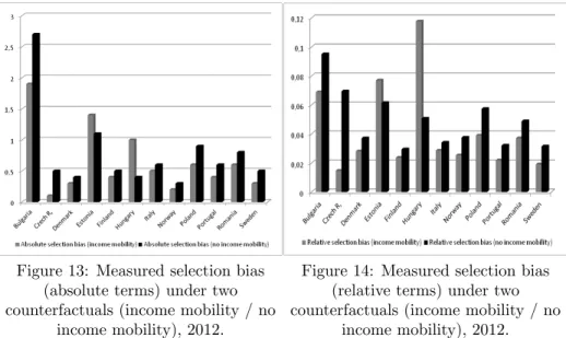
Figures 13 and 14 compare the sizes of measured selection biases (in absolute and relative terms) under the two counterfactuals (income mobility and no in-come mobility). Once we abstract from inin-come mobility, the measured selection bias due to income-di¤erentiated mortality becomes larger, except for Estonia and Hungary. Thus, in most countries, the presence of income mobility tends to reduce the size of the measured selection bias.
This illustrates the importance of the postulated counterfactual as far as the measurement of the selection bias is concerned. If one supposes that pre-maturely dead individuals would have, in case of survival, enjoyed the same income as the one they enjoyed at the time of dying, the measured selection bias in poverty measures is, in general, larger than when one assumes that prematurely dead individuals would have, in case of survival, faced the same income mobility process as the one faced by those who survived. The presence of income mobility tends to reduce the extent to which premature deaths can bias measures of poverty. Note, however, that there are some exceptions, such as Estonia and Hungary, for which the selection bias is higher under the income mobility counterfactual than under the no mobility counterfactual.
Figure 13: Measured selection bias (absolute terms) under two counterfactuals (income mobility / no
income mobility), 2012.
Figure 14: Measured selection bias (relative terms) under two counterfactuals (income mobility / no
5
Varying relative poverty lines
When measuring poverty, a crucial issue consists in the selection of a poverty line, below which individuals are counted as poor. Up to now, we used, for our calculations, a poverty line equal to 60 % of the median income in each country considered, the median income being computed on the basis of the income distribution prevailing before the adjustment is made. Note, however, that one may have used, as an alternative poverty line, a threshold equal to 60 % of the median income in each country on the basis of the income distribution prevailing after the adjustment is made. Indeed, adding missing persons in the income distribution is likely to a¤ect the level of the median income, and, hence, may also require to modify the poverty line.
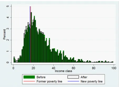
Once we allow for the adjustment of the poverty line to the new income dis-tribution, we obtain di¤erent corrected poverty rates. To illustrate this, Figure 15 shows, for the case of Bulgaria, the income distribution for the population aged 60 and more before and after the addition of missing persons, as well as the old and the new poverty lines. Given that the inclusion of missing persons adds more density on the left of the distribution (low income classes), the poverty line moves slightly to the left, which, in the case of Bulgaria, reduces the size of the adjustment of the poverty rate.
Figure 15: Income distribution (density) in Bulgaria (men and women aged 60+), 2012, before and after the addition of missing
persons. Old and new poverty lines.
mo-bility counterfactual, while assuming either the pre-adjustment poverty line or the post-adjustment poverty line.15
Relying on the new poverty threshold a¤ects the measured poverty in quite distinct ways across countries. Whereas this change in the poverty line has no e¤ect on the level of measured poverty in Portugal, this reduces signi…cantly the level of measured poverty in countries such as Bulgaria and Estonia. Note, however, that it remains true, whatever the poverty line that is used, that the addition of missing persons still inverts some international poverty rankings. Al-though Norway exhibits a higher poverty at age 60 + in comparison to Hungary in unadjusted terms, poverty is lower in Norway than in Hungary once the miss-ing persons are added, whatever we use the initial or the new poverty threshold. Thus, although adjusting the poverty line tends to reduce the corrected poverty rates, taking the missing persons into account has still a substantial impact on the measurement of old-age poverty.
Corrected poverty rate 60+ Corrected poverty rate 60+ (income mobility, initial threshold) (income mobility, new threshold) Countries Total Males Females Total Males Females
Bulgaria 27.6 22.8 31.5 25.7 20.9 29.7 Czech R. 6.8 4.9 8.4 6.6 4.9 8.1 Denmark 10.7 8.9 12.2 10.2 8.4 11.7 Estonia 18.2 15.6 19.7 15.6 13.0 17.2 Finland 16.9 14.0 19.3 16.7 13.7 19.2 Hungary 8.5 8.3 8.6 8.4 8.2 8.6 Italy 17.5 14.8 19.6 17.3 14.8 19.4 Norway 7.9 4.2 11.2 7.6 4.2 10.7 Poland 15.4 13.6 16.7 15.2 13.5 16.5 Portugal 18.3 17.0 19.3 18.3 17.0 19.3 Romania 16.2 13.1 18.6 16.0 13.0 18.3 Sweden 15.7 10.6 20.0 15.4 10.2 19.8
Table 6: Corrected poverty rates at age 60 + (under income mobility), initial and new poverty threshold (%), 2012.
As shown on Figure 16, the impact of changing the poverty line on the mea-sured selection bias induced by income-di¤erentiated mortality varies strongly across countries. In countries such as Finland, Hungary, Italy, Poland, Portugal and Romania, the selection bias remains positive and robust to the poverty line that is used. However, in Bulgaria, the selection bias, which was quite large under the past poverty line, vanishes to 0 under the new poverty line. In Es-tonia, the change is even larger: once the poverty line is adjusted to its new level, the addition of missing persons turns out not to increase, but to reduce the measured poverty.16
1 5See the Appendix for the new poverty lines.
1 6The reason for this surprising result lies in the fact that the income distribution in Estonia is such that there is a strong concentration of the population around the poverty line. Hence, a small decrease in the poverty threshold su¢ ces to cause a strong decrease in the measured poverty.
In sum, the robustness of the measured selection bias to the prevailing poverty line varies signi…cantly across countries. In some countries, adjust-ing the poverty line tends to strongly reduce the size of the measured selection bias, whereas there is little e¤ect in other countries. The same conclusion holds when considering the robustness of the relative selection bias (Figure 17).
Figure 16: Measured selection bias (absolute terms) under the old and the
new poverty lines, 2012.
Figure 17: Measured selection bias (relative terms) under the old and the
new poverty lines, 2012.
6
Absolute poverty line
Up to now, our analysis relied on a concept of relative poverty, in the sense that the poverty thresholds were assumed to be equal to 60 percents of the median income in each country under study. But one may also want to check whether the measure of the selection bias induced by income-di¤erentiated mortality is robust to the underlying concept of poverty. For that purpose, this section relies on a concept of absolute poverty. The poverty threshold is now assumed to be equal to 10 euros a day, adjusted for purchasing power parity (PPP).17
Table 7 presents the standard absolute poverty rates for the 12 countries under study, as well as the corrected poverty rates (while assuming income mobility as a counterfactual). Relying on a concept of absolute poverty yields a quite di¤erent picture of poverty in Europe, with poverty rates that are largely unequal across nations. Some countries, such as Bulgaria and Romania, exhibit
a high level of absolute old-age poverty (about 25 %), whereas other countries, such as the Nordic countries, exhibit poverty rates equal to less than 0.35 %.
Standard poverty rate 60+ Corrected poverty rate 60+ Countries Total Males Females Total Males Females
Bulgaria 24.8 17.8 27.0 26.6 21.8 30.6 Czech R. 0.47 0.51 0.43 0.45 0.48 0.42 Denmark 0.49 0.46 0.53 0.48 0.44 0.51 Estonia 3.33 3.49 3.23 3.57 3.89 3.37 Finland 0.16 0.22 0.11 0.16 0.23 0.11 Hungary 1.70 1.54 1.80 1.70 1.56 1.80 Italy 1.20 1.11 1.27 1.33 1.29 1.36 Norway 0.32 0.28 0.36 0.31 0.27 0.34 Poland 3.36 3.53 3.24 3.60 3.90 3.38 Portugal 2.53 2.71 2.41 2.81 3.13 2.56 Romania 29.56 24.11 33.58 30.69 25.97 34.38 Sweden 0.35 0.50 0.22 0.35 0.49 0.22
Table 7: Standard and corrected absolute poverty rates at age 60 + (%), 2012.
The extent to which adopting an absolute poverty line rather than a relative poverty line a¤ects the measured old-age poverty varies strongly across coun-tries. In order to illustrate this, Figures 18 and 19 show the adjustment of the income distributions in, respectively, Bulgaria and Norway, and the associated poverty rates under the relative and the absolute poverty lines. As far as Bul-garia is concerned (Figure 18), the absolute poverty line is close to the relative one, and the addition of missing persons implies the addition of a substantial density on the left of the two poverty lines. Hence, in the case of Bulgaria, the variation in the old-age poverty rate is robust to whether one uses a relative or an absolute poverty line. However, when considering Norway (Figure 19), it appears that the absolute poverty line is much more on the left than the relative poverty line. Only very low income classes are in absolute poverty in Norway. Given the small density of those low income classes, the adjustment of the in-come distribution leaves the absolute poverty rate quasi unchanged, unlike what we have under a relative poverty measure.
Figure 18: Income distribution (density) in Bulgaria (men and women aged 60+), 2012, before and after the addition of
missing persons. Absolute and relative poverty lines.
Figure 19: Income distribution (density) in Norway (men and women aged 60+), 2012, before and after the addition of
missing persons. Absolute and relative poverty lines.
There is a signi…cant heterogeneity across countries regarding the compari-son between standard and corrected poverty rates. In some countries, such as
Bulgaria, Estonia, Italy, Poland, Portugal and Romania, the corrected poverty rate is larger than the standard one, whereas in other countries, the addition of missing persons does not strongly a¤ect the level of the poverty rate. The strong heterogeneity across countries is also illustrated by Figure 20, which presents the relative selection bias for the 12 countries under study.
Figure 20: Measured selection bias (relative terms), measures of absolute poverty, 2012.
Comparing Figure 20 with Figure 10 reveals that shifting from a concept of relative poverty to a concept of absolute poverty a¤ects the picture signi…-cantly. Under a relative poverty line, all countries exhibited a positive selection bias measured in relative terms. However, under an absolute poverty line, the variance in the size of the measured relative selection bias is larger, with some countries exhibiting a zero (or even negative) relative selection bias.
7
Conclusions
Poor individuals exhibit higher mortality than non-poor individuals, implying some potential selection bias in old-age poverty estimates. This "missing poor" phenomenon has attracted substantial attention in the recent years, following the seminal paper by Kanbur and Mukherjee (2007). The extent to which the "missing poor" problem leads to more or less large selection biases in poverty measures depends on the hypothetical poverty rate that would have prevailed provided all individuals, poor or not, had faced the same survival conditions.
This paper proposed to cast new light on the "missing poor" problem, by paying particular attention to the design of counterfactuals that can be used to measure the selection bias due to income-di¤erentiated mortality. In particular, we wanted to examine here the role of the income mobility process. The intuition is that if there is strong upward income mobility, the prematurely dead persons (i.e. "missing persons") would, in case of survival, not have been so poor, so that the selection bias due to income-di¤erentiated mortality would then be
negligible. On the contrary, under strong downward income mobility, a large proportion of the non-poor "missing persons" would, in case of survival, have fallen into poverty, which would then lead to a larger selection bias.
In order to address that issue, we used data on poverty above age 60 in 12 European countries, and computed, for each country and gender, hypothetical poverty rates that would have prevailed if (i) all individuals, whatever their income, had enjoyed the same survival conditions (the ones of the highest income class), and if (ii) all individuals within the same income class had been subject to the same income mobility process. Those hypothetical poverty rates were then compared with the standard ones, to measure the size of the absolute and relative selection biases induced by income-di¤erentiated mortality.
Our main …nding is that measured selection biases are far from negligible, and that these di¤er strongly across countries and gender. A corollary of this is that selection biases a¤ect the comparison, in terms of old-age poverty, between countries and gender. A signi…cant part of di¤erences in old-age poverty rates across countries is due to selection biases (di¤erences in access to health care across countries), and is thus, in some sense, purely nominal. Moreover, in some countries, the poverty gender gap is much reduced once we correct for selection biases (because the income/mortality gradient is stronger for males, leading to larger selection bias in the measurement of old-age poverty among men). Thus taking selection e¤ects seriously matters for poverty measurement.
Another important result concerns the e¤ect of income mobility: when com-paring measured selection biases under the income mobility counterfactual with the ones under the no income mobility counterfactual, we see that biases are in general larger under the latter counterfactual. Thus income mobility tends to reduce measured selection bias, especially when upward income mobility is strong. In that case, many prematurely dead persons who were poor when being younger would have, in case of survival, escaped poverty. However, in Estonia and Hungary, the income mobility counterfactual leads to even larger old-age poverty than the no mobility counterfactual, since, in that case, many "missing persons" who were not poor when being younger would, in case of survival, have fallen into poverty. Income mobility has thus adverse e¤ects on the mea-surement of old-age poverty across countries. Thus taking income mobility - its strength and directions - into account when correcting poverty rates is essential to make accurate international comparisons of old-age poverty.
Our analyses also show that measured selection biases vary with the poverty line (pre- or post-adjustment, absolute or relative). Thus, in order to measure selection biases, the choice of a particular poverty line matters as much as the design of counterfactuals. Here again, there is a substantial heterogeneity across countries. Once we adopt an absolute poverty line, selection biases become small for Nordic countries, but remain substantial in Eastern Europe.
In sum, whereas the fact that mortality varies with income is well estab-lished, the precise quanti…cation of the missing poor phenomenon is far from trivial. Selection biases in old-age poverty measures vary with the underlying counterfactuals (in particular, the postulated income mobility) and also with the postulated poverty lines, to an extent that is far from uniform across countries.
8
References
Backlund, E., Sorlie, P. & Johnson, N. (1999) A comparison of the relationships of edu-cation and income with mortality: the national longitudinal mortality study. Social Science and Medicine, 49 (10): 1373-1384.
Bossert, W., Chakravarty, S.R. & D’Ambrosio, C. (2011) Poverty and time. Journal of Economic Inequality, 10 (2): 145-162.
Bossuyt, N., Gadeyne, S., Deboosere, P. & Van Oyen, H. (2004) Socio-economic inequal-ities in healthy expectancy in Belgium. Public Health 118:3–10
Deaton, A. & Paxson, C. (1998) Aging and inequality in income and health. American Economic Review, 88: 248-253.
Deaton, A. (2003) Health, inequality and economic development. Journal of Economic Literature, 41: 113-158.
Duggan, J., Gillingham, R. & Greenlees, J. (2007) Mortality and lifetime income: evidence from U.S. Social Security Records. IMF Working Paper, 07/15.
Duleep, H.O. (1986) Measuring the e¤ect of income on adult mortality using longitudinal administrative record data. Journal of Human Resources, 21 (2): 238-251.
Fields. G. & Ok, E. (1996) The Meaning and Measurement of Income Mobility. Journal of Economic Theory,71: 349-377.
Fields. G. & Ok, E. (1996) Measuring Movement of Incomes. Economica,66: 455-471. Foster, J. (2009) A class of chronic poverty measures. In: Addison, T., Hulme, D., Kanbur, R. (eds.) Poverty Dynamics: Interdisciplinary Perspectives, 59–76. Oxford University Press, Oxford.
Hoy, M. & Zheng, B. (2011) Measuring Lifetime Poverty. Journal of Economic Theory, 146 (6): 2544-2562.
Jantti, M. & Jenkins, S. (2015) Income Mobility. in A. B. Atkinson and F. Bourguignon (eds.) Handbook of Income Distribution, Vol 2. 807-935.
Jusot, F. (2004) Mortalité et revenu en France: construction et résultats d’une enquête cas-témoins. Santé, Société et Solidarité, 3 (2): 173-186.
Kanbur, R. & Mukherjee, D. (2007) Premature mortality and poverty measurement. Bul-letin of Economic Research, 59 (4): 339-359.
Lefebvre, M., Pestieau, P. & Ponthiere, G. (2013) Measuring Poverty Without the Mor-tality Paradox. Social Choice and Welfare, 40 (1): 285-316.
Lefebvre, M., Pestieau, P. & Ponthiere, G. (2017) FGT old age poverty measures and the Mortality Paradox: Theory and Evidence. Review of Income and Wealth, forthcoming.
Malthus, T. (1798) An Essay on the Principle of Population, London.
Pamuk E.R. (1985) Social class inequality in mortality from 1921 to 1972 in England and Wales. Population Studies, 39:17–31
Pamuk E.R. (1988) Social class inequality in infant mortality in England and Wales from 1921 to 1980. European Journal of Population 4:1–21
Salm, M. (2007) The e¤ect of pensions on longevity: evidence from Union Army veterans. IZA Discussion Paper 2668.
Schluter. C. & Van de gaer, D. (2011) Upward Structural Mobility. Exchange Mobility and Subgroup Consistent Mobility Measurement. US - German Mobility Rankings Revisited. Review of Income and Wealth, 57: 1-22.
Sen A.K. (1998) Mortality as an indicator of economic success and failure. Economic Journal 108:1–25
Van Kerm. P. (2004) What lies behind Income Mobility? Reranking and Distributional Change in Belgium. Western Germany and the USA. Economica 71. 223 - 239.
Van Kerm. P. (2009) Income Mobility Pro…les. Economics Letters 102. 93 - 95
Van Kerm P. & Alperin, M.N. (2013) Inequality, growth and mobility: The intertemporal distribution of income in European countries 2003–2007. Economic Modelling. vol. 35. pp. 931-939.
Van Oyen H., Bossuyt N., Deboosere P., Gadeyne S., Abatith E., & Demarest S. (2005) Di¤erential inequity in health expectancy by region in Belgium. Social Prevention Medicine 50(5): 301–310.
9
Appendix
9.1
Life expectancy by income class
This section presents the methodology that we use to extrapolate life expectancy by income classes from life expectancy by educational level (sources: EURO-STAT). The method consists in relating both distributions of individuals on the two dimensions (education and income). We estimate lifetables by income class using a weighted ordinary least square regression, as in Bossuyt et al (2004) and Van Oyen et al (2005) studies on health expectancy.
We start by transforming the absolute educational status into a relative educational status. In education lifetables provided by EUROSTAT, a three-category classi…cation is used: 1) primary education or less; 2) secondary edu-cation and 3) higher eduedu-cation. The eduedu-cational attainment is used to de…ne a social position that will be related to the level of income.
Among cohorts, the size of educational groups has changed. Young peo-ple studied more than older ones, so that the corresponding income level may have changed. Furthermore, since the education sector varies from one country to another, using a relative concept allows the comparison. Figure A1 shows the method. The horizontal axis represents the distribution of a hypothetical population according to education. Each form below the axis is an education category. The …rst one represents the % of people with at most a primary degree, the second one is the % of people with a secondary education degree and the third one is the tertiary education. Thus we represent each category of education by its size in the population and order these categories from the lowest level to the highest on a scale from 0 to 100%. That is each category of education represents a percentage of the population. This scale gives us a distribution of the cohort population according to education.
Figure A1: Mid-point references for education categories.
We assume that the reference of an education category is determined by its relative position, de…ned as the mid-point of the proportion of the category represented on the ordered scale of 100% (Pamuk, 1985, 1988). For example, if the …rst category is given by those with at most a primary degree and rep-resents 18% of the cohort, the mid-point reference will be 9%. If those with a secondary degree represent 54% of the population, the bounds of the category in the distribution are 18 and 72% and the mid-point is 45%.
Once we have determined the position of each category of education on the scale, the life expectancy of each category is associated to the point. We regress the life expectancy by education on the reference mid-point of the education category by weighting for the prevalence of the category, i.e. the relative size of the educational level. The slope of the regression line represents the di¤erence in mortality between the bottom and the top of the education hierarchy. Table A1 presents the estimation results for the population aged 65 and for each country and sex separately.
Dependent variable: Life expectancy
Bulgaria Czech R. Denmark Estonia Finland Hungary Men Constant 11.805 12.776 16.738 12.605 16.925 13.032 Mid-point 0.057 0.065 0.019 0.052 0.021 0.047 R2 0.863 0.855 0.997 0.941 0.966 0.565 Women Constant 15.883 18.388 19.674 19.477 21.220 17.411 Mid-point 0.037 0.019 0.017 0.019 0.010 0.022 R2 0.869 0.604 0.873 0.995 0.977 0.680
Dependent variable: Life expectancy
Italy Norway Poland Portugal Romania Sweden Men Constant 17.562 17.373 13.951 16.552 13.771 17.821 Mid-point 0.025 0.023 0.033 0.023 0.022 0.016 R2 0.828 0.903 0.861 0.862 0.682 0.995 Women Constant 21.750 20.308 19.287 20.899 17.391 20.502 Mid-point 0.011 0.019 0.014 0.011 0.012 0.015 R2 0.784 0.921 0.741 0.629 0.688 0.993
Table A1 : Mid-point regression of life expectancy by education –age 65 Once estimated, the coe¢ cients can be used to compute life table according to income. This is done by assuming that the social hierarchy given by the income is similar to the one given by education. Here we assume that there are 100 di¤erent income categories of equal amount and we assume that both education and income give the same social hierarchy. These categories can obviously change from one country to another. In order to obtain life expectancy by income category, we can thus apply the coe¢ cient of one education category to the corresponding categories of income.
The categories of income change from a country to another, this to re‡ect the actual distribution of income. We consider 99 categories of 100 euros and the last one is residual in Bulgaria, Poland and Romania. Categories of 150 in Hungary. Categories of 200 euros in Czech R., 400 euros in Portugal, 500 euros in Denmark, Finland, Italy and Sweden and 800 euros in Norway.
9.2
Income mobility matrices
Bulgaria - men cl 1 cl 2 cl 3 cl 4 cl 5 cl 6 cl 7 cl 8 cl 9 cl 10 cl 1 52.92 39.81 5.11 0.95 0.55 0.00 0.26 0.00 0.00 0.40 cl 2 6.99 58.49 26.53 5.71 1.02 0.68 0.22 0.16 0.10 0.11 cl 3 1.32 14.06 51.99 24.84 5.52 1.32 0.37 0.31 0.09 0.18 cl 4 0.66 4.64 21.96 45.47 18.08 5.64 1.86 0.75 0.16 0.76 cl 5 0.07 2.01 9.56 25.43 38.52 14.46 5.27 2.58 0.97 1.15 cl 6 0.08 1.58 4.45 16.60 25.55 28.88 14.40 4.79 1.91 1.75 cl 7 0.16 2.13 5.25 9.02 16.39 21.89 19.92 11.56 8.44 5.25 cl 8 0.24 0.73 2.18 5.81 7.38 19.85 22.76 19.13 9.69 12.23 cl 9 0.39 0.00 6.04 6.82 5.85 9.94 14.23 13.45 19.69 23.59 cl 10 0.00 2.98 5.64 4.86 5.02 13.17 10.03 11.91 12.07 34.33Table A2: Matrix of income mobility across classes (%) for 2012 - men aged 60+, Bulgaria Bulgaria - women cl 1 cl 2 cl 3 cl 4 cl 5 cl 6 cl 7 cl 8 cl 9 cl 10 cl 1 46.47 45.41 5.77 1.35 0.68 0.03 0.21 0.00 0.00 0.09 cl 2 6.32 64.07 22.87 4.63 1.08 0.54 0.18 0.13 0.08 0.10 cl 3 1.31 14.74 51.95 23.93 5.67 1.40 0.37 0.31 0.10 0.23 cl 4 0.72 4.88 22.15 44.75 18.15 5.61 1.77 0.96 0.29 0.72 cl 5 0.00 2.13 9.90 25.72 38.55 14.28 5.14 2.37 0.98 0.93 cl 6 0.35 1.87 4.80 14.95 27.51 26.90 13.30 5.23 2.35 2.75 cl 7 0.18 2.27 4.71 7.80 17.04 24.48 17.86 11.24 9.52 4.90 cl 8 0.37 0.99 2.85 6.95 6.82 16.25 25.19 18.73 9.80 12.03 cl 9 0.18 0.00 5.10 4.75 5.80 10.54 13.53 13.71 22.14 24.25 cl 10 0.00 2.38 5.35 4.46 4.61 17.53 8.47 10.40 15.16 31.65
Table A3: Matrix of income mobility across classes (%) for 2012 - women aged 60+, Bulgaria
Czech Republic - men
cl 1 cl 2 cl 3 cl 4 cl 5 cl 6 cl 7 cl 8 cl 9 cl 10 cl 1 9.29 57.14 9.29 17.86 1.43 4.29 0.00 0.00 0.00 0.71 cl 2 2.03 39.53 43.35 10.63 2.39 1.24 0.24 0.21 0.00 0.36 cl 3 0.11 4.91 51.49 36.26 5.68 0.89 0.24 0.23 0.12 0.07 cl 4 0.01 1.30 11.33 57.50 23.72 4.22 1.22 0.28 0.11 0.30 cl 5 0.00 0.50 3.29 19.21 48.96 20.75 4.98 1.23 0.13 0.96 cl 6 0.00 0.32 1.30 6.52 23.18 39.87 19.25 5.97 1.77 1.83 cl 7 0.00 1.04 1.23 5.64 12.23 19.10 34.24 18.71 4.41 3.41 cl 8 0.00 0.00 0.67 4.83 6.91 11.81 18.55 28.95 16.14 12.15 cl 9 0.00 0.00 1.60 3.33 7.07 10.40 6.67 14.67 25.87 30.40 cl 10 0.00 0.00 0.64 5.89 3.32 5.68 6.43 8.47 14.58 54.98
Table A4: Matrix of income mobility across classes (%) for 2012 - men aged 60+, Czech Republic.
Czech Republic - women cl 1 cl 2 cl 3 cl 4 cl 5 cl 6 cl 7 cl 8 cl 9 cl 10 cl 1 2.74 52.74 13.01 23.97 4.11 2.05 0.00 0.00 0.00 1.37 cl 2 1.05 39.54 48.01 8.21 1.76 0.67 0.18 0.28 0.12 0.18 cl 3 0.11 4.91 58.15 30.98 4.60 0.70 0.21 0.18 0.07 0.08 cl 4 0.01 1.18 12.31 57.62 22.86 4.13 1.24 0.28 0.10 0.27 cl 5 0.00 0.54 3.82 20.56 47.38 20.55 5.11 1.05 0.14 0.84 cl 6 0.00 0.18 1.37 6.98 22.59 39.64 20.08 5.43 1.50 2.22 cl 7 0.00 0.71 0.80 5.30 12.15 21.48 33.33 19.08 3.99 3.15 cl 8 0.00 0.00 0.46 3.24 6.49 13.07 19.18 28.45 16.68 12.42 cl 9 0.00 0.00 1.67 4.25 8.50 9.10 8.35 16.54 22.15 29.44 cl 10 0.00 1.56 1.44 3.83 3.23 6.10 5.86 6.22 14.95 56.82
Table A5: Matrix of income mobility across classes (%) for 2012 - women aged 60+, Czech Republic. Denmark - men cl 1 cl 2 cl 3 cl 4 cl 5 cl 6 cl 7 cl 8 cl 9 cl 10 cl 1 17.14 17.14 48.57 8.57 0.00 5.71 2.86 0.00 0.00 0.00 cl 2 1.75 41.98 36.15 9.33 7.87 1.46 0.58 0.87 0.00 0.00 cl 3 0.33 3.58 60.05 27.81 6.47 1.12 0.28 0.23 0.00 0.14 cl 4 0.08 0.69 6.82 60.44 26.02 4.11 1.20 0.10 0.15 0.38 cl 5 0.00 0.36 1.06 11.09 56.28 25.67 3.98 0.73 0.36 0.48 cl 6 0.00 0.17 0.77 1.80 13.01 55.47 22.66 4.29 1.03 0.80 cl 7 0.06 0.15 0.61 1.87 4.40 15.92 49.10 21.49 4.46 1.95 cl 8 0.11 0.38 0.33 0.49 2.58 7.25 15.93 45.25 19.60 8.07 cl 9 0.00 0.00 0.13 0.26 2.95 6.28 8.08 17.95 33.97 30.38 cl 10 0.00 0.11 0.74 0.85 4.02 3.81 5.07 7.51 11.73 66.17
Table A6: Matrix of income mobility across classes (%) for 2012 - men aged 60+, Denmark. Denmark - women cl 1 cl 2 cl 3 cl 4 cl 5 cl 6 cl 7 cl 8 cl 9 cl 10 cl 1 16.67 20.83 25.00 16.67 0.00 8.33 0.00 0.00 0.00 12.50 cl 2 0.27 48.40 33.16 9.63 6.15 1.07 0.53 0.00 0.00 0.80 cl 3 0.16 3.19 61.64 26.47 6.13 1.47 0.37 0.16 0.08 0.33 cl 4 0.04 0.61 5.89 63.80 23.96 3.88 1.23 0.13 0.21 0.25 cl 5 0.01 0.24 1.22 11.09 56.89 24.91 4.07 0.79 0.24 0.55 cl 6 0.05 0.24 0.69 2.06 13.15 54.13 23.54 4.38 0.79 0.96 cl 7 0.06 0.18 0.33 2.14 3.98 16.23 50.27 20.62 4.57 1.63 cl 8 0.00 0.11 0.29 1.03 3.04 7.51 15.59 44.36 20.74 7.34 cl 9 0.00 0.41 0.28 0.55 2.07 7.02 7.30 16.67 35.95 29.75 cl 10 0.00 0.53 1.17 1.27 3.82 3.50 4.56 7.00 11.03 67.13
Table A7: Matrix of income mobility across classes (%) for 2012 - women aged 60+, Denmark.
Estonia - men cl 1 cl 2 cl 3 cl 4 cl 5 cl 6 cl 7 cl 8 cl 9 cl 10 cl 1 22.35 42.35 27.06 1.18 1.18 1.18 1.18 0.00 1.18 2.35 cl 2 2.66 40.84 42.31 9.25 2.93 0.73 0.09 0.37 0.46 0.37 cl 3 0.53 9.15 52.72 28.00 7.07 1.62 0.48 0.07 0.02 0.33 cl 4 0.16 1.68 9.97 53.86 27.58 5.36 0.99 0.17 0.06 0.17 cl 5 0.13 0.59 2.42 16.10 51.45 23.71 4.15 1.06 0.27 0.13 cl 6 0.23 0.41 1.48 4.39 21.03 42.94 22.49 4.83 1.22 0.98 cl 7 0.00 0.34 1.09 1.37 6.03 22.43 39.84 21.80 4.85 2.24 cl 8 0.62 0.79 0.96 1.47 2.54 6.44 22.59 32.41 21.74 10.45 cl 9 0.14 0.54 0.82 1.77 1.36 3.81 6.81 21.53 27.93 35.29 cl 10 0.11 1.19 0.00 0.87 0.87 0.65 4.22 7.58 15.69 68.83
Table A8: Matrix of income mobility across classes (%) for 2012 - men aged 60+, Estonia. Estonia - women cl 1 cl 2 cl 3 cl 4 cl 5 cl 6 cl 7 cl 8 cl 9 cl 10 cl 1 10.17 38.98 33.90 5.08 5.08 1.69 0.00 0.00 1.69 3.39 cl 2 1.33 41.05 41.49 11.17 2.75 1.15 0.27 0.18 0.27 0.35 cl 3 0.36 7.84 59.16 24.52 5.78 1.56 0.48 0.12 0.02 0.16 cl 4 0.14 1.74 10.17 55.78 26.05 4.83 0.93 0.14 0.09 0.12 cl 5 0.26 0.67 2.50 16.11 51.19 23.31 4.62 1.03 0.21 0.10 cl 6 0.20 0.61 1.76 4.34 19.73 42.82 23.66 4.93 1.15 0.81 cl 7 0.06 0.35 1.29 1.23 5.59 21.88 40.28 22.38 4.39 2.56 cl 8 0.61 0.97 0.97 1.45 2.48 6.55 22.85 33.52 20.85 9.76 cl 9 0.14 0.42 0.71 1.27 1.84 4.39 5.38 22.38 29.75 33.71 cl 10 0.12 1.08 0.48 0.72 0.96 1.08 4.57 7.45 14.66 68.87
Table A9: Matrix of income mobility across classes (%) for 2012 - women aged 60+, Estonia. Finland - men cl 1 cl 2 cl 3 cl 4 cl 5 cl 6 cl 7 cl 8 cl 9 cl 10 cl 1 16.15 43.85 24.62 10.00 1.54 1.54 0.77 0.00 1.54 0.00 cl 2 2.74 44.79 38.74 9.26 2.37 1.05 0.26 0.37 0.26 0.16 cl 3 0.20 6.15 56.49 28.90 5.80 1.47 0.55 0.26 0.15 0.04 cl 4 0.22 1.82 10.56 54.23 25.68 5.09 1.25 0.70 0.24 0.20 cl 5 0.07 0.72 2.26 14.37 52.85 22.56 5.08 1.22 0.38 0.50 cl 6 0.00 0.89 1.74 4.44 15.99 46.84 21.65 5.83 1.59 1.03 cl 7 0.12 0.58 1.49 1.76 6.57 17.40 41.55 22.04 5.57 2.92 cl 8 0.00 0.61 0.61 1.60 2.55 5.94 19.64 35.54 23.28 10.25 cl 9 0.00 1.65 0.52 1.19 2.38 3.83 8.17 18.56 31.95 31.75 cl 10 0.28 0.66 1.13 1.84 1.25 1.41 3.28 4.00 9.47 76.68
Table A10: Matrix of income mobility across classes (%) for 2012 - men aged 60+, Finland