HAL Id: hal-00643664
https://hal.inria.fr/hal-00643664
Submitted on 22 Nov 2011HAL is a multi-disciplinary open access archive for the deposit and dissemination of sci-entific research documents, whether they are pub-lished or not. The documents may come from teaching and research institutions in France or abroad, or from public or private research centers.
L’archive ouverte pluridisciplinaire HAL, est destinée au dépôt et à la diffusion de documents scientifiques de niveau recherche, publiés ou non, émanant des établissements d’enseignement et de recherche français ou étrangers, des laboratoires publics ou privés.
Michel Batteux, Philippe Dague, Nicolas Rapin, Philippe Fiani
To cite this version:
Michel Batteux, Philippe Dague, Nicolas Rapin, Philippe Fiani. Diagnosability study of technological systems. 24th International Conference on Industrial, Engineering and other Applications of Applied Intelligent Systems IEA/AIE 2011, Jun 2011, Syracuse, United States. �hal-00643664�
K.G. Mehrotra et al. (Eds.): IEA/AIE 2011, Part I, LNAI 6703, pp. 186–198, 2011. © Springer-Verlag Berlin Heidelberg 2011
Michel Batteux1, Philippe Dague2, Nicolas Rapin3, and Philippe Fiani1
1
Sherpa Engineering, La Garenne Colombe, France {m.batteux,p.fiani}@sherpa-eng.com 2
LRI, Univ. Paris-Sud & CNRS, INRIA Saclay – Île-de-France, Orsay, France [email protected]
3
CEA, LIST, Laboratory of Model driven engineering for embedded systems, Point Courier 94, Gif-sur-Yvette, 91191, France
Abstract. This paper describes an approach to study the diagnosability of
technological systems, by characterizing their observable behaviors. Due to the interaction between many components, faults can occur in a technological system and cause hard damages not only to its integrity but also to its environment. Though a diagnosis system is a suitable solution to detect and identify faults, it is first important to ensure the diagnosability of the system: will the diagnosis system always be able to detect and identify any fault, without any ambiguity, when it occurs? In this paper, we present an approach to identify and integrate faults in a model of a technological system. Then we use these models for the diagnosability study of faults by characterizing their observable behaviors.
Keywords: faults modeling, diagnosability, model-based diagnosis.
1 Introduction
Technological systems are complex systems constituted with many components interacting with each other and combining multiple physical phenomena: thermodynamic, hydraulic, electric, etc. Faults, which are un-observable damages affecting components of a system, can occur due to many causes: wear, dirtying, breakage, etc. Some are serious and must require to stop the system, or to put it in a safety mode; while others have minor impact and should only be reported for being repaired off-board. Thus, it is necessary to achieve on-board the detection of these faults and to identify them the most precisely; this in order to take the appropriate decision. An embedded diagnosis system, completing the controller, is a suitable solution to do this ([1]). However, the problem is then to ensure that this diagnosis system will always be able not only to detect any fault when it occurs (does the fault induce an observable behavior distinct from the normality?), but also to assign a unique listed fault to a divergent observable behavior (do some faults induce the same observable behavior?). This problem is known as diagnosability ([2]).
A way to handle this diagnosability, with respect to a system, is to augment the model of this system (the normal model) with faults (producing faulty models); and to exploit them to characterize observable behaviors of the system, under or not a fault,
by a specific property which will be verified by the diagnosis system. This approach, called diagnosability study of faults, inheres in the analysis process of the diagnosis system. It requires, by definition, all faulty models to produce, for each one, a specific fault characterization according to its observable behaviors. All these faults characterizations will then be used by the embedded diagnosis system to detect and identify faults.
In this paper, we present an approach to study the diagnosability of faults of a technological system by exploiting its observable behaviors. These observable behaviors are obtained by using the normal and all faulty models of the system. In the second part, we present the framework to model a technological system and show how to integrate faults in it. In the third part, we exploit these produced models in order to define observable behaviors of the system in the normal and all faulty cases. In the fourth part, we study diagnosability of faults by producing their characterizations. In the fifth part, we apply this theoretical framework to a practical application: a fuel cell system. Finally, the last part concludes by summarizing results and outlining interesting directions for future works.
2 System and Faults Modeling
In order to study faults diagnosability of a system, it is necessary to get the normal model and all faulty models of the system. In this part, we present the framework to obtain a model of a system and show how to integrate faults into it.
2.1 Normal Model of the System
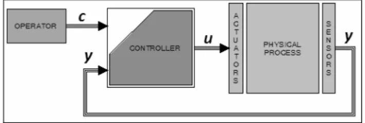
Classical works found in literature for diagnosis ([1], [3] and [4]) are based on a representation of the system in open-loop. But for the majority of industrial applications, the system is inserted in a closed-loop and its controller computes system inputs by taking into account its outputs; this to increase system performances and to maintain them in spite of unknown perturbations affecting it. In this context fault detection and isolation are more difficult because of the contradiction between control objectives and diagnosis objectives. In fact, control objectives are to minimize disturbances or faults effects; whereas diagnosis objectives are precisely to bring out these faults. The considered solution, to take into account this problem, is to model the system with its controller in closed-loop. Fig. 1 below represents the complete structure of the system: the system and its controller in closed-loop.
We model a controlled system with two parts: the controller and the system itself composed of the physical process, actuators and sensors. We consider a continuous model in discrete time T with a state space representation, described by the set (1) of equations:
x(t+1) = f(x(t),θ,u(t),d(t)), x(0) = xinit
y(t) = g(x(t),θ,u(t),d(t)) a(t+1) = h(c(t),a(t),y(t)), a(0) = ainit
u(t) = k(c(t),a(t),y(t))
(1)
where the two first equations model the system and the two other ones model the controller (more precisely its control laws). Variables u, x, θ, d and y are respectively input, state, parameter, disturbance and output vectors of the system; c and a are respectively order (from the operator) and state vectors of the controller. We denote by V = {c;a;u;x;y;d} the set of all variables of the model, with respective domains of values C, A, U, X, Y and D, and by VObs = {c;u;y} the set of observable variables. 2.2 Faults Modeling
Faults in the system can cause failures or malfunctions, resulting in serious damages not only to the system integrity but also to its environment. It is therefore important to identify and classify all potential faults of the system in order to ensure their integration in the model.
By using methodologies of safety engineering ([5] and [4]), an identification of all important faults of the system can be made. Thanks to faults analysis techniques, such as Failure Mode and Effects Analysis or Fault Tree Analysis, we can identify most of potential faults which could occur in the system; and analyze their causes and impacts. Therefore, the set Γ = {F0,F1,…,Fk} of potential faults, that must be taken
into account by a diagnosis system, is identified and defined during this safety analysis, where to simplify the presentation, the fault F0 represents the normal case.
Potential faults can be classified in order to ensure their integration in the model. Various classifications of faults can be found in literature ([1], [4] and [6]); but all of them differentiate the behavior of the fault and its effects on the system ([7]). Fault behavior is characterized by its occurrence time (randomly, at a specific time or from a specific event), its appearance (abruptly or progressively) and its form (permanent, transient or intermittent). Fault effects consist in its location inside the system and its disturbance induced. For our purpose, we do not consider faults occurring in the controller. Thus, there are sensor faults (perturbing the output vector y), actuator faults (perturbing the input vector u) and faults in the process (perturbing the state vector x or the parameter vector θ). The disturbance can be additive, multiplicative, sinusoidal or limitative.
Thus, for a fault F∈Γ\{F0} and a time instant tn∈T, the faulty model of the system
under F is obtained by considering the set of equations (1) where the considered disturbed variable v is replaced by its disturbance vF = dist(t,v(t),flt(t,tn)), with flt the
fault behavior and tn∈T its occurrence time. For example with a sensor fault F,
represented by yF(t) = dist(t,y(t),flt(t,tn)), the faulty model of the system is described
x(t+1) = f(x(t),θ,u(t),d(t)), x(0) = xinit
y(t) = dist(t,g(x(t),θ,u(t),d(t)),flt(t,tn))
a(t+1) = h(c(t),a(t),y(t)), a(0) = ainit
u(t) = k(c(t),a(t),y(t))
(2)
3 Observable Behaviors
By adding faults in the model of the system, we have produced all faulty models requested for the diagnosability study. We can now exploit them to characterize observable behaviors in the normal and all faulty cases. A behavior of the system represents its way of operation, according to an instruction (a sequence of orders) from the operator. An observable behavior is therefore obtained from the behavior by restricting it to the only observable variables. Observable means visible from an external observer, such as a diagnosis system for example.
3.1 System Behaviors
A behavior of the system is represented by the set of values of variables during its operation and according to an instruction from the operator. This operation can be under the presence, or not, of a fault. A behavior is therefore specified according to an instruction and a fault.
An instruction is the evolution of orders from the operator during the time. Formally, it is a sequence cs from a temporal window Ics ⊆ T, assumed beginning
from the time instant 0, to the domain C. In the following, we consider a set Cons of instructions the most representative, i.e.: providing all operation ranges of the system. Thus, though each instruction cs is defined from its own temporal window Ics, we
assume that all instructions are defined from a same temporal window I = max{Ics},
by extending any instruction cs, where Ics ⊂ I, with its last value cs(max(Ics)).
For a vector v = (v1,…,vn) and for an index i ∈{1,…,n}, we denote by pi(v) = vi the
i-th element of v. For a set E, constituted by a direct product E = E1×…×En, for a
sub-set G ⊆ E and for indexes i1,…,ik ∈{1,…,n} with k ≤ n ; the projection of G onto the
k i i E E × × 1 is the set PrEi1× ×Eik(G) ={( ( ), , ( ) 1 v p v p k i i )∈Ei1× ×Eik\ v∈G}.
Normal Behaviors.For an instruction cs∈Cons, the normal behavior of the system, according to cs, is the set B(cs,F0) of vectors of data (t,v(t))∈I×C×A×U×X×Y×D,
ordered by time t, with v(t) = (c(t),a(t),u(t),x(t),y(t),d(t)). This set of data vectors satisfies the following:
a. Existence and uniqueness in time: for any time instant t∈I, it exists a unique vector v(t)∈C×A×U×X×Y×D such as (t,v(t))∈B(cs,F0).
b. Construction according to the instruction cs: for any time instant t∈I,
p1(v(t)) = cs(t).
c. Satisfaction of system equations in normal case: for any time instant t∈I, 1. p4(v(t+1)) = f(p4(v(t)),θ,p3(v(t)),p6(v(t))) and p4(v(0)) = xinit
3. p2(v(t+1)) = h(p1(v(t)),p2(v(t)),p5(v(t))) and p2(v(0)) = ainit
4. p3(v(t)) = k(p1(v(t)),p2(v(t)),p5(v(t)))
Faulty Behaviors.A characteristic of faults behaviors, defined in the above part, is the occurrence time (randomly, at a specific time, or from a specific event). In the following, we only consider faults occurring at a specific time; in fact our focus is only to ensure diagnosability of a fault when it occurs, not to predict its occurrence. Thus, for each fault F∈Γ\{F0} and each instruction cs∈Cons, we consider a set Ω(F,cs)
of time occurrence tn∈I of the fault F according to the instruction cs.
Therefore, for an instruction cs∈Cons and a fault F∈Γ\{F0} occurring at a time
instance tn∈Ω(F,cs), the faulty behavior of the system B(cs,F,tn) is defined as the
normal one above where points (c) is replaced with the satisfaction of system equations in the considered faulty case.
3.2 Observable Behaviors of the System
An observable behavior of the system represents its visible, from an external observer, way of operation according to an instruction from the operator. It is obtained by projecting the behavior, according to the considered instruction, onto the set of observable variables.
In addition, detection and isolation of a fault require, for industrial applications, to be made in bounded time b after the fault occurrence. This bound can be assumed more than the response time δ of the system. Thus, as a behavior could be defined for a fault occurring at the time instant tn = max(I), it could not consider onto the time
interval [tn,tn+b] as it is not defined. Therefore, for any fault F∈Γ\{F0} and any
instruction cs∈Cons, we only consider time occurrences
tn∈Θ(F,cs) = Ω(F,cs) ∩ [0;max(I) – b]. F0 can be considered as a fault always occurring
at the time instant tn = 0; thus, Θ(Fo,cs) = {0} for any instruction cs∈Cons.
For a faulty behavior B(cs,F,tn), according to an instruction cs∈Cons and under a
fault F∈Γ\{F0} occurring at a time instance tn∈Θ(F,cs), the underlying faulty
observable behavior ObsB(cs,F,tn) is the projection of B(cs,F,tn) onto the direct
product I×C×U×Y of observable variables: ObsB(cs,F,tn) = PrI×C×U×Y(B(cs,F,tn)).
For a normal behavior B(cs,F0), according to an instruction cs∈Cons, and the time
instant tn∈Θ(Fo,cs) (={0}), the underlying normal observable behavior ObsB(cs,F0,tn) is
the projection of B(cs,F0) onto the direct product I×C×U×Y of observable variables: ObsB(cs,F0,tn) = PrI×C×U×Y(B(cs,F0)). The parameter tn, which is always equal to 0, is
added to harmonize with the notation of faulty observable behaviors ObsB(cs,F,tn).
An observable behavior is defined according to an instruction cs∈Cons, a fault
F∈Γ and an occurrence time tn∈Θ(F,cs) (tn = 0 for F0). Therefore the set of observable
behaviors, according to the set Cons of instructions and under a fault F∈Γ, is the union of all observable behaviors for all instructions cs of Cons and all occurrence time tn∈Θ(F,cs) of F: ObsBehCons(F)=∪cs∈Cons∪tn∈Θ(F,cs){ObsB(cs,F,tn)}. Finally, the set of observable behaviors, according to the set Cons of instructions, is the union of all sets of observable behaviors for all faults: ObsBehCons = ∪F∈ΓObsBehCons(F). We also
define the time domain Tdom(ob) of an observable behavior ob∈ObsBehCons as I and a
set J = [b;max(I)] ⊂ I.
4 Diagnosability Study of the System
Intuitively a fault F∈Γ\{F0} is said diagnosable if observable behaviors of the system
under this fault are not the same that observable behaviors of the system under another fault F’∈Γ\{F}. This other fault can be F0, or another one F’∈Γ\{F0;F},
which expresses the two ideas: the fault detectability and the fault isolability.
The diagnosability study inheres in the analysis process of the diagnosis system. In fact, during its operation, the diagnosis system will check if the observed behavior of the system, provided by data of observable variables, satisfies a specific property characterizing the normal operation of the system. If this property is not satisfied, it will search which property, characterizing an abnormal operation, is satisfied. Consequently, the diagnosability study will be made from a set Λ = (PF)F∈Γ of
properties characterizing the most precisely observable behaviors of the system under the considered fault. Λ is said a faults characterization.
4.1 Faults Characterization
For a fault F∈Γ, its characterization is a property PF which must be satisfied at each
time instant by at least observable behaviors under this considered fault (PF : ObsBehCons×J→{true;false}). We propose two kinds of faults characterization. The Perfect Characterization (PC). The most natural solution to characterize observable behaviors is to consider them restricted to the temporal windows [t – b;t], with b the bound presented above.
- For the fault F0∈Γ, the set of bounded normal observable behaviors is
ObsBehbdCons(F0) = ∪cs∈Cons∪t∈J{Pr[t-b;t]×C×U×Y(ObsB(cs,F0,0))}.
- For a fault F∈Γ\{F0} the set of bounded faulty observable behaviors is
ObsBehbdCons(F) = t t [t ;t ] ) , ( n b Cons cs∈ ∪ ∈ΘFcs ∪∈ n n+ ∪ {Pr[t-b;t]×C×U×Y(ObsB(cs,F,tn))}.
For a fault F∈Γ, its perfect characterization is the property PF defined as follow: for
an observable behavior ob∈ObsBehCons and a time instant t∈J, PF(ob,t) is true iff Pr[t–
b;t]×C×U×Y(ob)∈ObsBehbdCons(F).
Intuitively, an observable behavior ob∈ObsBehCons, restricted to a temporal
window [ti – b;ti], is an element of the set ObsBehbdCons(F) iff it exists an instruction
cs∈Cons, an occurrence time tn∈Θ(F,cs) of F and a time instant td∈[tn;tn+b], such as
data vectors of ob (which are restricted to the temporal window [ti – b;ti]) are equal to
data vectors of ObsB(cs,F,tn) restricted to the temporal window [td – b;td]. I.e., if for
any time instant k∈[0;b] ⊆ T, the data vector v(ti+k) of ob at the time instant ti+k is
equal to the data vector v’(td+k) of ObsB(cs,F,tn) at the time instant td+k.
It is a perfect characterization because it is not possible to specify, in a best way, observable behaviors. In fact, the sets ObsBehbdCons(F), constructed by restricting
elements of ObsBehCons(F), are the nominal definitions of observable behaviors of the
system under a fault; it is therefore not possible to do it better. Nevertheless, not only the set Cons of instructions must be the most representative: the set CI of all functions from the temporal window I to the domain C; but also all sets Θ(F,cs) of occurrence
time of faults must be equal to J.
The Temporal Formulas Characterization (TFC). This faults characterization describes how the system operates under a fault thanks to a temporal formula. We will use an adaptation of the metric interval temporal logic ([8]), well adapted to specify bounded real-time properties.
The syntax of temporal formulas is classically defined by induction. The set of terms, representing arithmetic formulas, is built from the set VObs={c;u;y} of
observable variables of the system, a set Κ of constants, arithmetic operators (+, −, ⋅ and ÷) and a temporal operator V[α], where α∈T is a positive or negative time instant.
Atomic formulas, expressing a comparison (equality or inequality) between two arithmetic formulas, are built from the set of terms and by using comparison operators (=, ≠, <, >, ≥ and ≤). Temporal formulas are therefore built, recursively, with operators ¬ (not), ∧ (and) G[α;β] (globally during a temporal window bounded by α
and β) and E[α;β] (eventually during a temporal window bounded by α and β); where
α,β∈T are two positive or negative time instants. Classical operators ∨ (or) and ⇒ (implication) and ⇔ (equivalent) are built from the above operators ¬ and ∧.
Temporal formulas are interpreted by observable behaviors ob∈ObsBehCons at each
time instant t∈J: the satisfaction of ϕ by ob at the time instant t, denoted by (ob,t)╞ ϕ, is classically defined by induction onto the set of temporal formulas:
- (ob,t)╞ atom, iff t∈Dom(atom) = Tdom(ob) and atom is true when all observable variables are replaced by their values from the vector of ob at the time instant t. If
atom contains a term of the form V[α]v, its satisfaction is obtained if
t+α∈Dom(atom) and by considering the value of v at the time instant t+α. - (ob,t)╞ ¬ϕ iff t∈Dom(ϕ) and (ob,t) does not satisfy ϕ.
- (ob,t)╞ ϕ ∧ ψ iff t∈Dom(ϕ)∩Dom(ψ) and (ob,t)╞ ϕ and (ob,t)╞ ψ.
- (ob,t)╞ G[α;β]ϕ iff [t+β;t+α]⊆Dom(ϕ) and for all t’ in [t+β;t+α] we have
(ob,t’)╞ ϕ (if [t–β;t–α]⊄Dom(ϕ) the value of G[α;β]ϕ is not defined).
- (ob,t)╞ E[α;β]ϕ iff [t+β;t+α]⊆Dom(ϕ) and there exists t’ in [t+β;t+α] such that
(ob,t’)╞ ϕ (if [t–β;t–α]⊄Dom(ϕ) the value of E[α;β]ϕ is not defined).
For example, the formula ϕex: G[-3;0]( (c∈[0;1[) ∧ (c – V[-0.1]c = 0) ), where c∈[0;1[
means (0 ≤ c) ∧ (c < 1), asserts that since 3 time units, the variable c is in the interval [0;1[ and has not changed.
Fault Characterization Formulas. All data sets ObsBehCons(F) of observable behaviors
under a fault are obtained by simulation. By analyzing them, for each fault F∈Γ, a specific temporal formula ϕF is generated.
The normal formula ϕFo consists in checking thresholds of the gap |c – y| according
- Firstly, ϕFo is divided into sub-formulas ϕiFo according to a partition C = Ui∈ECi of
the domain C. This partition represents all operating points of the system. Thus, when the order c is in a part Ci, the sub-formula ϕiFo is checked.
- Secondly, each sub-formula ϕiFo is divided into two sub-formulas: a sub-formula
ϕi,h
Fo for high changes of order; and another ϕi,lFo for low changes. For a high
change of order, more than a threshold, the sub-formula ϕi,hFo is checked from the
time of the change and during the response time δ of the system. Otherwise, for low changes of order less than the threshold, the sub-formula ϕi,lFo is checked.
All faulty formulas are elaborated by taking into account behaviors and effects of faults. Thus, these characteristics are transformed, if it is possible, into temporal formulas describing how the fault disturbs the gap |c – y| and all observable variables
u and y.
For a fault F∈Γ, its temporal formula characterization is the property PF defined as
follow: for an observable behavior ob∈ObsBehCons and a time instant t∈J, PF(ob,t) is
true iff (ob,t)╞ ϕF. Temporal formulas are checked, thanks to the ARTiMon© tool,
from the CEA, LIST ([9]), interfaced to MATLAB/Simulink©.
4.2 Diagnosability Study
Whatever is the considered faults characterization Λ = (PF)F∈Γ, we can give a general
definition of diagnosability. Although we have presented two kinds of such characterizations (PC and TFC); another kind could be used.
Formal definitions. Given a faults characterization Λ = (PF)F∈Γ, a fault F∈Γ is said
diagnosable if it is eligible, detectable and isolable.
- A fault F∈Γ is eligible iff for any instruction cs∈Cons and for any occurrence time tn∈Θ(F,cs) of F (tn = 0 for F0), it exists a time instant te∈[tn;tn+b] such that for all time
instant t∈J with t ≥ te: PF(ObsB(cs,F,tn),t) is true.
- A fault F∈Γ\{F0} is detectable iff for any instruction cs∈Cons and for any
occurrence time tn∈Θ(F,cs), it exists a time instant td∈[tn;tn+b] such that for all time
instant t∈J with t ≥ td: PFo(ObsB(cs,F,tn),t) is false.
- A faultF∈Γ\{F0} is isolable iff for any instruction cs∈Cons and for any occurrence
time tn∈Θ(F,cs), it exists a time instant ti∈[tn;tn+b] such that for all time instant t∈J
with t ≥ ti: PF’(ObsB(cs,F,tn),t) is false for any other fault F’∈Γ\{F0;F}.
Analysis According to the Kind of Characterization. We have defined the diagnosability for any faults characterization Λ = (PF)F∈Γ; we can therefore point up
some remarks.
The diagnosability is defined for all faults F∈Γ; thus for F0, there is just to check
its eligibility. Furthermore, this eligibility notion is added because as it is defined for any faults characterization Λ, it could be possible to consider one where some faults are not eligible. Obviously, it is not the case with PC: by definition of all sets
Since the diagnosability is defined by the conjunction of three notions, we could study them independently. But in practical applications for example the isolability study of a fault F∈Γ\{F0} will be considered only if F is detectable and with respect
to other detectable faults F’∈Γ\{F0;F}. In fact, if a fault is not detectable for the
diagnosability study, it means that it will not be detected by the diagnosis system when it will occur. This is due to the fact that the diagnosability study inheres in the analysis process of the diagnosis system.
We can observe a useful result: if a fault is not diagnosable with PC, it will not be diagnosable with TFC. In fact, TFC is obtained by exploiting the data sets
ObsBehCons(F), thus it can be considered as a reduction of these sets. TFC is therefore
a reduction of PC and its diagnosability requirements are thus stronger.
A brief complexity analysis shows the advantage of using TFC for an embedded diagnosis system.
- Space complexity: first, at each tk sample, the diagnosis system has to store the
received observable data vector. In addition, it has to keep only previous required data vectors during a temporal window bounded according to the considered faults characterization: the bound b for PC and β for TFC (the size of the longest temporal window appearing in all formulas). Thus, it is a number nPerf = #v · (b/u) for PC and
nForm = #v · (β/u) for TFC, where u is the time unit (e.g.: u = 0.01) and #v is the
number of observable variables. Then, the diagnosis system must store all formulas for TFC; whereas all data sets ObsBehbdCons(F) for PC. It means a number of data
mForm = nForm + ΠF∈Γ(2h(F)) for TFC and m = ΣF∈Γ(Σcs∈Cons(mF,cs)) for PC (where h(F)
is the level of the formula F, mFo,cs = (#J · nPerf) and mF,cs = (#Θ(F,cs) · (b/u) · nPerf), #J
is the number of time instants between b and max(I) and #Θ(F,cs) is the number of
time occurrences F according to cs).
- Time complexity: for each tk sample the embedded diagnosis system must check the
real observed behavior of the system during a temporal window of operation, according to the considered faults characterization, against all data of observable behavior previously stored, also according to the kind of faults characterization. This time complexity is therefore proportional to the space complexity.
Therefore, PC could not be exploited by an embedded diagnosis system. First, the diagnosis system should have enough memory to store all these data sets
ObsBehbdCons(F) for each fault F∈Γ, and enough computational power to make all
comparisons. Second, as we have seen, the set Cons of instructions must be the most representative: the set CI of all functions from I ⊆ T to C. Therefore this solution would be unusable for complex system with large ranges of operation. Nevertheless, it is useful during design and development phases of the system to intrinsically ensure the diagnosability of faults identified during the safety analysis.
Finally, TFC is perfectly adapted to be embedded inside a diagnosis system. In fact, conception and development phases are actually more and more accomplished with simulation tools which are able to generate the source code of control laws
directly for a controller. We could add the embeddable ARTiMon© technology
(involved in the diagnosability study), with all temporal formulas, during the source code generation; it will be the embedded diagnosis system completing the controller.
5 Practical Applications
With the above theoretical framework, we have defined the diagnosability study of faults by analyzing their observable behavior obtained by models. By using
simulation tools, such as MATLAB/Simulink©, we can apply this theoretical
framework in practical applications.
First of all, we require a simulation model of the system. Simulation models used in control design could be a first solution; nevertheless, as showed in [10], we have to keep in mind that models needed for diagnosis are not the same that models needed for control. A model for control is generally less complex than a model for diagnosis.
We assume to have a simulation model of the system (the process and its controller) and furthermore we assume the model of the process represents perfectly the real system.
5.1 A Simulation Model Example
For example, we consider a part of a simulation model, developed in Matlab/Simulink©, of a fuel cell system embedded in an electric vehicle ([7]). The concerned part is the air alimentation line of the fuel cell stack. To summarize, thanks to a compressor at the beginning and a valve at the end of the line, this air line has to provide air to the fuel cell stack at specific mass flow rates and pressures supplied by the global controller of the fuel cell system. This model can be described, in a simplified manner for the system part, by the set (3) of equations:
P(t+1) = k(Qin(t) – Qout(t)), P(0) = 1 Qin(t) = fin(W(t),P(t)) Qout(t) = fout(X(t),P(t)) W(t) = αW · uW(t) X(t) = αX · uX(t) yP(t) = λP · P(t) yQ(t) = λQ · Qin(t) (3)
P is the air pressure in the line. Qin and Qout are air mass flow rates respectively
before and after the stack. W is the compressor speed rotation and X is the valve opening. uW and uX are respectively compressor and valve orders from the air line
controller; yP and yQ are respectively air pressure and air mass flow rate measures. k,
αW, αX, λP, λQ are constants.
These mass flow rate and pressure are controlled according to orders (cQ for mass
flow rate and cP for pressure) supplied by the global controller of the fuel cell system.
The supplied mass flow rate order cQ is computed, for the most part, according to the
electrical power needed by the vehicle controller (the operator). The pressure order cP
is then deduced from this mass flow rate according to pressure requirements in the stack and in the line. Thus, we can assume the mass flow rate order cQ is the main
order. Therefore, the set of observable variables of this air line is
All important faults of the air line have been identified and integrated in the simulation model by using an adapted faults library developed in MATLAB/Simulink© ([7]). For example, we consider a lock of the compressor Flock
which causes an abrupt decrease of the mass flow rate output of the compressor; and during the fault presence, this mass flow rate output stays equal to 0 gram per second. Within the model, variable Qin is therefore disturbed by a multiplicative perturbation
and is described by Qin,Flock(t) = (1 – flt(t,tn)) · Qin(t), where flt is the behavior of Flock,
parameterized to occur abruptly at a time instant tn and stay permanent (so flt(t,tn) = 0
before tn and 1 after).
5.2 Observable Behaviors Obtained by Simulations
We have considered a set Cons of instructions representing all operation ranges of the air line. By simulating the normal and all faulty models, according to the set Cons of instructions, we have obtained all data sets ObsBehCons(F) of observable behaviors for
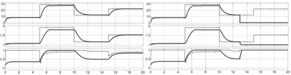
all identified faults F∈Γ parameterized according to their behaviors and effects ([7]). Fig. 2 illustrates two observable behaviors obtained for a random instruction cs during the temporal window [0;20]. In the two figures, first and second graphs show the mass flow rate and the pressure in the air line: dotted lines represent orders cQ and
cP whereas plain lines represent measures yQ and yP from sensors. The third graph
shows orders from the air line controller: compressor orders uW in plain line and valve
orders uX in dotted line. Fig. 2 on left shows the normal observable behavior
ObsB(cs,F0,0) whereas Fig. 2 on right shows the faulty observable behavior ObsB(cs,Flock,13), for the lock of the compressor occurring at the time instant 13.
During the time interval [0;13[, the air line operates correctly, as the normal behavior; but from the time instant 13, we can see disturbances in all graphs. Mass flow rate measures (first graph) decrease abruptly to 0 gram per second; compressor orders (third graph) are therefore maximal (equal to 1) in order to compensate the difference between orders and measures. Pressure measures (second graph) are thus equal to 1 bar.
5.3 Results on the Air Line Model
The diagnosability study of faults in the air line model was achieved with use of the temporal formulas characterization.
For example, the conjunction ϕFo, of the two following formulas, characterizes the
observable behavior of the air line in the normal case: ϕ1 Fo: (cQ∈[0;25[) ⇒ ( ( G[-3;0](c – V[-0.01]c = 0) ⇒ ( (|cQ – yQ| ≤ 0.5) ∧ (|cP – yP| ≤ 0.1) ) ) ∨ ( E[-3;0](c – V[-0.01]c ≠ 0) ⇒ ( (|cQ – yQ| > 0) ∧ (|cP – yP| > 0) ) ) ) ϕ2 Fo: (cQ∈[25;30]) ⇒ ( ( G[-3;0](c – V[-0.01]c = 0) ⇒ ( (|cQ – yQ| ≤ 1) ∧ (|cP – yP| ≤ 0.5) ) ) ∨ ( E[-3;0](c – V[-0.01]c ≠ 0) ⇒ ( (|cQ – yQ| > 0) ∧ (|cP – yP| > 0) ) ) )
Fig. 2. Observable behaviors obtained by simulations (left: normal; right: lock of compressor)
The following formula ϕlock characterizes the observable behavior of the air line
under the lock of the compressor:
ϕlock: ( G[-1;0]( ( yQ = 0 ) ∧ ( yP = 1 ) ∧ ( uW = 1 ) ∧ ( uX = 1 ) ) )
We consider the set of faults Γ = {F0;Flock}, where F0 is the normal case and Flock is
the lock of the compressor only occurring at the time instant tn = 13. We suppose the
set Cons of instructions is reduced to {cs} and we consider a bound b = 5. Thus,
ObsBeh{cs} = {ObsB(cs,F0,0);ObsB(cs,Flock,13)}, with Θ(Fo,cs) = {0} and
Θ(Flock,cs) = {13}.
Firstly, the normal observable behavior ObsB(cs,F0,0) satisfies the formula ϕFo.
Therefore, the fault F0 is eligible.
Secondly, the faulty observable behavior ObsB(cs,Flock,13) satisfies the faulty
formula ϕlock from the time instant te = 14,3∈[13;18]; therefore, the fault Flock is
eligible. In addition, from the time instant 13, this faulty observable behavior
ObsB(cs,Flock,13) does not satisfy the normal formula ϕ0; the fault Flock is therefore
detectable.
Of course, it is just an example. Firstly, the set of instructions is not reduced to only one but contains several ones representing all operation ranges of the system. Moreover, all identified faults have been taken into account with several occurrence times: before or after a change of orders and according the response time δ of the system. Furthermore all real temporal formulas obtained are more elaborated.
6 Conclusions and Perspectives
In this paper, our goal was to exploit faulty models of a technological system to study faults diagnosability. We have first presented the theoretical framework to define observable behaviors of a system under, or not, a fault. It considers a model of the system with its controller and integrates faults, preliminary identified and classified, in this model. Then, according to a set of instructions representing all operation ranges of the system, we have defined observable behaviors in the normal and all faulty cases. They consist in sets of vectors of observable data ordered by time according to a given instruction of the set of instructions.
The notion of faults diagnosability was defined regardless of a considered faults characterization, describing, the most precisely, how the system operates under or not a fault. Two faults characterizations were proposed. A perfect one, well adapted for
the study during design and development phases of the system, simply considers all sets of data vectors, restricted to temporal windows. The other one uses temporal logic formalism to express the temporal evolution of observable data of the system and is adapted for an embedded diagnosis system.
Finally, for diagnosable faults, their characterization will then be embedded inside the diagnosis system in order to detect and identify faults on line. It could be combined with an embedded model of the system simulated by the controller and temporal formulas could take into account the temporal evolution of the difference between real and model outputs data. These future works will be presented in forthcoming papers.
References
1. Venkatasubramanian, V., Rengaswamy, R., Yin, K., Kavuri, S.N.: A review of process fault detection and diagnosis. ’part I to III’. Computers and Chemical Engineering 27, 293–346 (2003)
2. Travé-Massuyès, L., Cordier, M.O., Pucel, X.: Comparing diagnosability in CS and DES. In: International Workshop on Principles of Diagnosis, Aranda de Duero, Spain, June 26-28 (2006)
3. Blanke, M., Kinnaert, M., Lunze, J., Staroswiecki, M.: Diagnosis and Fault-tolerant Control. Springer, Berlin (2003)
4. Isermann, R.: Fault Diagnosis Systems. Springer, Berlin (2006)
5. Stapelberg, R.F.: Handbook of Reliability, Availability, Maintainability and Safety in Engineering Design. Springer, London (2009)
6. Basseville, M., Nikiforov, I.V.: Detection of Abrupt Changes: Theory and Application. Prentice-Hall, Englewood Cliffs (1993)
7. Batteux, M., Dague, P., Rapin, N., Fiani, P.: Fuel cell system improvement for model-based diagnosis analysis. In: IEEE Vehicle Power and Propulsion Conference, Lille, France, September 1-3 (2010)
8. Alur, R., Feder, T., Henzinger, T.A.: The Benefits of Relaxing Punctuality. Journal of the ACM 43, 116–146 (1996)
9. Rapin, N.: Procédé et système permettant de générer un dispositif de contrôle à partir de comportements redoutés spécifiés, French patent n°0804812 pending, September 2 (2008) 10. Frank, P.M., Alcorta García, E., Köppen-Seliger, B.: Modelling for fault detection and
isolation versus modelling for control. Mathematics and Computers in Simulation 53(4-6), 259–271 (2000)