Convex modeling with priors

Convex Modeling with Priors

by

Benjamin Recht

B.S., University of Chicago (2000)

M.S., Massachusetts Institute of Technology (2002)

Submitted to the Media Arts and Sciences

in partial fulfillment of the requirements for the degree of

Doctor of Philosophy

at the

MASSACHUSETTS INSTITUTE OF TECHNOLOGY

June 2006

@

Massachusetts Institute of Technology 2006. All rights reserved.

Author ... . .. .... ... U BR

Media Arts and Sciences

A

April 14, 2006

Certified by...

Neil Gershenfeld

Associate Professor

Thesis Supervisor

&41

A ccepted by ...

...

...

....

.. ...

Andrew B. Lippman

Chairman, Departmental Committee on Graduate Students

MASSACHUSETTS INSTE

OF TECHNOLOGY

JUN 0 9 2006

ZARIES

Convex Modeling with Priors

by

Benjamin Recht

Submitted to the Media Arts and Sciences on April 14, 2006, in partial fulfillment of the

requirements for the degree of Doctor of Philosophy

Abstract

As the study of complex interconnected networks becomes widespread across disciplines, modeling the large-scale behavior of these systems becomes both increasingly important and increasingly difficult. In particular, it is of tantamount importance to utilize available prior information about the system's structure when building data-driven models of complex behavior. This thesis provides a framework for building models that incorporate domain specific knowledge and glean information from unlabelled data points.

I present a methodology to augment standard methods in statistical regression with

priors. These priors might include how the output series should behave or the specifics of the functional form relating inputs to outputs. My approach is optimization driven: by for-mulating a concise set of goals and constraints, approximate models may be systematically derived. The resulting approximations are convex and thus have only global minima and can be solved efficiently. The functional relationships amongst data are given as sums of nonlinear kernels that are expressive enough to approximate any mapping. Depending on the specifics of the prior, different estimation algorithms can be derived, and relationships between various types of data can be discovered using surprisingly few examples.

The utility of this approach is demonstrated through three exemplary embodiments. When the output is constrained to be discrete, a powerful set of algorithms for semi-supervised classification and segmentation result. When the output is constrained to follow Markovian dynamics, techniques for nonlinear dimensionality reduction and system identi-fication are derived. Finally, when the output is constrained to be zero on a given set and non-zero everywhere else, a new algorithm for learning latent constraints in high-dimensional data is recovered.

I apply the algorithms derived from this framework to a varied set of domains. The dissertation provides a new interpretation of the so-called Spectral Clustering algorithms for data segmentation and suggests how they may be improved. I demonstrate the tasks of tracking RFID tags from signal strength measurements, recovering the pose of rigid objects, deformable bodies, and articulated bodies from video sequences. Lastly, I discuss empirical methods to detect conserved quantities and learn constraints defining data sets.

Thesis Supervisor: Neil Gershenfeld Title: Associate Professor

Convex Modeling with Priors by Benjamin Recht PhD Thesis Signature Page Thesis Advisor ... ... * ... Neil Gershenfeld Associate Professor Department of Media Arts and Sciences Massachusetts Institute of Technology

T hesis R eader ...

John Doyle John G. Braun Professor Departments ofonyrql and Dynamical Systems, Electrical Engineering, and BioEngineering Califo ia Institute of Technology

Thesis Reader ... . ...

1-ablo Parrilo

Associate Professor Department of Electrical Engineering and Computer Science Massachusetts Institute of Technology

Acknowledgments

I would first like to thank the members of my committee for providing invaluable guidance

and support. My advisor, Neil Gershenfeld, encouraged me to pursue my diverse interests and provided a stimulating environment in which to do so. John Doyle took me under his wing and introduced me to the wide world of robustness. Pablo Parrilo shared his many insights and creative suggestions on this document and on the score of papers we still have left in the queue.

The work in this thesis arose out of a long-running collaboration with Ali Rahimi. Most of the results contained herein are distilled from papers we have written together or ideas composed in late nights of brainstorming and coding (with some bickering). I'd like to thank him for such a fruitful collaboration. This document benefited from a careful reading by Ryan Rifkin who provided many useful comments and corrections. Aram Harrow suggested a simple proof of Theorem 4.2.4. Along with being my co-conspirator on the Audiopad project, James Patten provided the hardware and his time for the acquisition of the Sensetable data in Chapter 5. Andy Sun and Jon Santiago assisted in the collection of the Resistofish data also discussed in Chapter 5. Kenneth Brown, Bill Butera, Constantine Caramanis, Waleed Farahat, Tad Hirsch, and Dan Paluska also provided helpful feedback. I'd especially like to thank Raffaello D'Andrea for his friendship and mentorship during my graduate career. I'd like to thank everyone else I have collaborated with during my stay at MIT including Ethan Bordeaux, Isaac Chuang, Brian Chow, Chris Csikszentmihalyi, Trevor Darrell, Saul Griffith and Squid Labs, Hiroshii Ishii, Seth Lloyd, Cameron Marlow, Jim McBride, Ryan McKinley, Ravi Pappu, Jason Taylor, Noah Vawter, Brian Whitman, and the students of the MIT Media Lab. I have learned more in these collaborations with my peers than anywhere else in my graduate career. I would also like to acknowledge my other fellow travellers in the Physics and Media Group: Rich F., Ara K., Raffi K., Femi 0., Rehmi P., Manu P., Matt R., Amy S., and Ben V.

None of this work would have been possible without the diligent staff of the CBA office.

I'd like to thank Susan Murphy-Bottari, Kelly Maenpaa, and Mike Houlihan for all of their

help, hard work, and support. I also extend my gratitude to Linda Peterson and Pat Solakoff in the MAS office for making it easier to leap over the hurdles that accompany the graduate school process.

My involvment in the Boston electronic music scene has served as an important

coun-terpoint to and release from my academic work. Notable shout outs go to The Fun Years, The Dan Bensons Project, Mike Uzzi, The Saltmine, Unlockedgroove, The DSP Music Syndicate, The Appliance of Science, non-event, Beat Research, Spectrum, Jake Trussell, Anthony Flackett, Collision, Don Mennerich, Eric Gunther, Fred Giannelli, and Stewart Walker. We are the reason Boston is the drone capital of the universe.

Of course, I am deeply indebted to Mom and Dad for their endless support. I'd like to

thank my sister Marissa for putting up with my bad attitude longer than any reasonable person would have. And finally, I'd like to thank Lauren, without whom I would have probably finished this thesis, but it wouldn't have been half as good.

This work was supported in part by the Center for Bits and Atoms (NSF CCR-0122419), ARDA/DTO (F30602-30-2-0090), and the MITRE Corporation (0705N7KZ-PB).

Contents

1 Introduction

1.1 Contributions and Organization . . . . 1.2 N otation . . . . . . . .. 2 Mathematical Background 2.1 Basics of Convexity . . . . 2.1.1 Convex Sets.... . . . . . . . . . .. 2.1.2 Convex Functions . . . . 2.1.3 Convex Optimization . . . . 2.2 Convex Relaxations . . . . 2.2.1 Nonconvex Quadratically Constrained Quadratic Programming 2.2.2 Applications in Combinatorial Optimization . . . .

2.3 Reproducing Kernel Hilbert Spaces and Regularization Networks . . . 2.3.1 Lessons from Linear Regression . . . .

2.3.2 Reproducing Kernel Hilbert Spaces . . . .

2.3.3 The Kernel Trick and Nonlinear Regression . . . .

3 Augmenting Regression with Priors

3.1 Duality and the Representer Theorem ...

3.2 Augmenting Regression with Priors on the Output. 3.2.1 Least-Squares Cost . . . .

3.2.2 The Need for Constraints . . . . 3.2.3 Priors on the Output . . . .

21 23 24 27 27 27 28 31 34 36 40 47 49 51 53 57 . . . . 58 . . . . 63 . . . . 64 . . . . 66 . . . . 68

3.2.4 Semi-supervised and Unsupervised Learning . . . . 3.3 Augmenting Regression with Priors on Functional Form . . . . . 3.3.1 The Dual of the Arbitrary Regularization Problem . . . 3.3.2 A Decomposition Algorithm for Solving the Dual Problem Kernel Learning . . . . 3.3.3 Example 1: Finite Set of Kernels . . . . 3.3.4 Example 2: Gaussian Kernels . . . . 3.3.5 Example 3: Polynomial Kernels . . . .

and

3.4 Conclusion... . . . . . . . .. 4 Output Prior: Binary Labels

4.1 Transduction, Clustering, and Segmentation via constrained outputs . 4.2 RKHS Clustering is NP-HARD . . . . 4.3 Semidefinite Approximation using Lagrangian Duality . . . . 4.4 Eigenvalue Approximations and the Normalized Cuts Algorithm . . . 4.4.1 The Normalized Cuts Algorithm. . . . . .. 4.4.2 Average Gap Algorithm . . . . 4.5 Numerical Experiments. . . . . . . . .. 4.6 Conclusion . . . . 5 Output Prior: Dynamics

5.1 Related Work . . . . 5.2 Model for Semi-Supervised Nonlinear System ID . 5.2.1 Semi-supervised Algorithm . . . . 5.2.2 Unsupervised Algorithm . . . . 5.3 Relation to System Identification . . . . 5.4 Interactive Tracking Experiments . . . . 5.4.1 The Dynamics Model . . . . 5.4.2 Synthetic Results . . . . 5.4.3 Interactive Tracking . . . . 5.4.4 Calibration of HCI Devices . . . .

107 . . . . 108 . . . . 110 . . . . 115 . . . . . . . 117 . . . . 118 . . . . 119 . . . . 120 . . . . 120 . . . . 123 . . . . 124 71 72 73 75 76 78 80 83 85 87 90 94 98 99 101 103 105

5.4.5 Electric Field Imaging:.... . . . . . . .. 5.5 Conclusion... . . . . . . . . . . . ..

6 Output Prior: Manifolds of Low Codimension 6.1 Learning Manifolds of Low Codimension . . . 6.2 Basis Functions and Polynomial Models . . . . 6.3 Lifting to a General RKHS . . . . 6.4 Null Spaces and Learning Surfaces . . . . 6.5 Choosing a Basis . . . .... 6.6 Learning Manifolds . . . .

7 Conclusion

A Linear Algebra

A.1 Unconstrained Quadratic Programming . . . .

A.2 Schur Complements . . . .

A.3 More Quadratic Programming . . . . A.4 Inverting Partitioned Matrices . . . . A.5 Schur complement Lemma . . . . A.6 Matrix Inversion Lemma . . . . A.7 Lemmas on Matrix Borders . . . .

B Equality Constrained Norm Minimization on Product Space an Arbitrary Inner 155 129 131 135 136 137 138 139 141 141 145 149 149 150 150 151 151 152 152 . . . . . . . . . . . . . . . . ... . . . ... .. ..

List of Figures

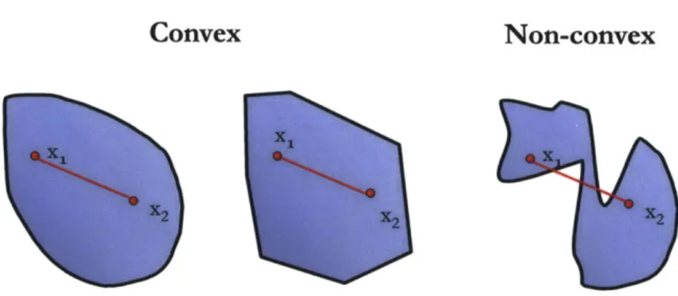
2-1 Left and Middle: Two convex sets. In each set a line segment is drawn between two points in the set and this line never leaves the set. Right:

A nonconvex set. Two points are shown which cannot be connected by a

straight line that doesn't leave the set. . . . . 28

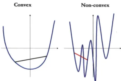
2-2 Left: A convex function. One can readily check that the area above the blue curve contains all line segments between all points. Right: The red

segment demonstrates that the region above the graph is not convex. . . . 30

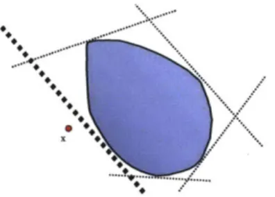
2-3 The convex set is separated from the points not in the set by half-spaces. The bold dashed line separates the plane into two halves, one containing the point x and the other containing the convex set. . . . . 31

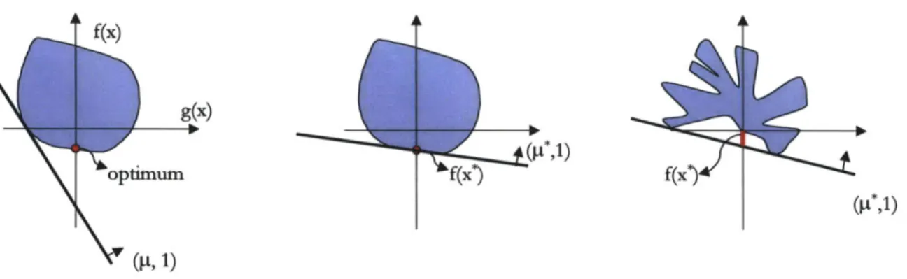
2-4 The set of possible pairs of g(x) and f(x) are shown as the blue region. Left: Any hyperplane which has normal (p, 1) intersects the y-axis at the point

f(x*) - PTg(x*) where x* minimizes C(x, t) with respect to x. Middle:

A hyperplane whose y intercept is equal to the minimum of f(x) on the

feasible set. The dual optimal value is equal to that of the primal Right: No hyperplane can achieve the primal optimal value. The discrepancy between the primal and dual optima is called a duality gap. The dual optimum value is always a lower bound for the primal. . . . . 34

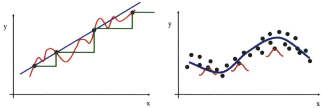
2-5 Left: Given four point, a variety of exact fits are shown. A prior on the function is required to make the problem well-posed. Right: Regularization Networks place a "bump" at each observed data point to fit unseen data. . 47

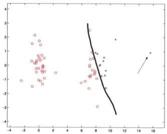
4-1 In Normalized Cuts, an outlier can dwarf the influence of other points, because points away from the mean are heavily weighted. Sliding the outlier (indicated by the arrow) along the x-axis can shift the clustering boundary arbitrarily to the left or the right. Without the outlier, Normalized Cuts places the boundary between the two clusters. . . . . 102

4-2 Because Normalized Cuts puts more weight on points away from the mean, it prefers to have the ends of the elongated vertical cluster on opposite sides of the separating hyperplane . . . . . 102

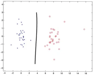
4-3 The data set of Figure 4-1 is correctly segmented by weighting all points equally. The outlier point doesn't shift the clustering boundary significantly. 104

4-4 The data set of Figure 4-2 is correctly segmented by weighting all points equally. . . . . 104

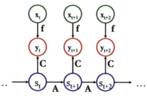
5-1 A generative model for a linear system with nonlinear output. The states st

are low-dimensional representations lifted to high dimensional observables xt by an embedding g... . . . . . . . . 118

5-2 Forcing agreement between projections of observed xt and a Markov chain of states st. The function

f

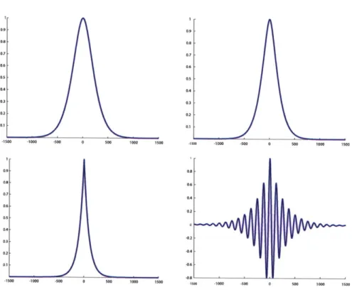
maps observations to outputs of a linear system. 119

5-3 The covariance between samples over time for various (A, C) pairs. The x-axis represents number of samples from -1500 to 1500. The y-axis shows covariance on a relative scale from 0 to 1. (top-left) Newtonian dynamics model used in the experiments. (top-right) Dynamics model using zero ac-celeration. (bottom-left) Brownian Motion model. (bottom-right) A second order model with oscillatory modes. . . . . 121

5-4 (top-left) The true 2D parameter trajectory. Semi-supervised points are marked with big black triangles. The trajectory is sampled at 1500 points (small markers). Points are colored according to their y-coordinate on the manifold. (top-middle) Embedding of a path via the lifting F(x, y) =

(x,

Iy|,

sin(iry)(y2 + 1)-2 + 0.3y). (top-right) Recovered low-dimensional representation using our algorithm. The original data in (top-left) is cor-rectly recovered. (bottom-left) Even sampling of the rectangle [0, 5] x [-3, 3]. (bottom-middle) Lifting of this rectangle via F. (bottom-right) Projection of (bottom-middle) via the learned function g. g has correctly learned the mapping from 3D to 2D. These figures are best viewed in color. . . . . . 122

5-5 (left) Isomap's projection into R2 of the data set of Figure 5-4(top-middle). Errors in estimating the neighborhood relations at the neck of the manifold cause the projection to fold over itself. (right) Projection with BNR, a semi-supervised regression algorithm. There is no folding, but the projections are not close to the ground truth shown in Figure 5-4(top-left)... . . . . . 122

5-6 The bounding box of the mouth was annotated for 5 frames of a 2000 frame

video. The labelled points (shown in the top row) and first 1500 frames were used to train our algorithm. The images were not altered in any way before computing the kernel. The parameters of the model were fit using leave-one-out cross validation on the labelled data points. Plotted in the second row are the recovered bounding boxes of the mouth for various frames. The first three examples correspond to unlabelled points in the training set. The tracker is robust to natural changes in lighting, blinking, facial expressions, small movements of the head, and the appearance and disappearance of teeth. . . . . 125

5-7 The twelve supervised points in the training set for articulated hand tracking

5-8 The hand and elbow positions were annotated for 12 frames of a 2300 frame video. The labelled points (shown in Figure 5-7) and the first 1500 frames were used to train our algorithm. The images were not preprocessed in any way. Plotted in white are the recovered positions of the hands and elbows. Plotted in black are the recovered positions when the algorithm is trained without taking advantage of dynamics. Using dynamics improves tracking significantly. The first two rows correspond to unlabelled points in the training set. The last row correspond to frames in the last 800 frames of the video, which was held out during training. . . . . 126

5-9 An image of the Audiopad. The plot shows an example stream of antenna resonance information. Samples from the output of the Sensetable over a six second period, taken over the trajectory marked by large circles in the left panel . . . . . 129

5-10 (left) The ground truth trajectory of the tag. The tag was moved around

smoothly on the surface of the Sensetable for about 400 seconds, produc-ing about 3600 signal strength measurement samples after downsamplproduc-ing. Triangles indicate the four locations where the true location of the tag was provided to the algorithm. The color of each point is based on its y-value, with higher intensities corresponding to higher y-values. (right) (middle) The recovered tag positions match the original trajectory. (right) Errors in recovering the ground truth trajectory. Circles depict ground truth loca-tions, with the intensity and size of each circle proportional to the Euclidean distance between a points true position and its recovered position. The largest errors are outside the bounding box of the labelled points. Points in the center are recovered accurately, despite the lack of labelled points there. 130

5-11 Once f is learned, it can be used it to track tags. Each panel shows a ground

truth trajectory (blue crosses) and the estimated trajectory (red dots). The recovered trajectories match the intended shapes.... . . . .. 130

5-12 (left) Tikhonov regularization with labelled examples only. The trajectory is

not recovered. (middle) BNR with a neighborhood size of three using nearest neighbors. (right) BNR with same neighborhood settings, with the addition of temporal neighbors. There is folding at the bottom of the plot, where black points appear under the red points, and severe shrinking towards the

mean... . . . . . . . 131

5-13 The Resistofish senses humans by detecting the low-level electric fields that

couple them to ground. The hand couples capacitively to a resistive sheet with electrodes on the sides. The time constant of the RC pair that couple the hand to the sheet are measured by undersampling timing the impulse response of a voltage change at each electrode . . . . . 132

5-14 The resistive sheet and the two dollar sensor that make up the Resistofish hardware. . . . . 132

5-15 Two different algorithms were used to measure the mapping from the RC

time constants to the position of the hand. (left) A sample trajectory. (middle) The recovered trajectory under the supervised algorithm. (left) The recovered trajectory by the unsupervised regression algorithm. Note that the trajectory is rotated, but the geometry is correctly recovered. . . 132

5-16 The top row is recovered using the supervised algorithm. The bottom row

is recovered by the unsupervised algorithm. The middle panels is the re-covered traces of someone writing "MIT." The right-most panels are the recovered traces of someone writing "Ben." The mapping recovered by the unsupervised algorithm is as useful for tracking human interaction as the mapping recovered by the fully calibrated regression algorithm. . . . . 133

6-1 The SPHERE data set. 200 points were sampled from a gaussian with unit variance and then normalized to have length 1. This sampling procedure generates a uniform distribution on the sphere. . . . . 142

6-2 The first four figures show the zero-contours of four functions whose coeffi-cients span the null-space of lifted data for SPHERE. The final figure shows the intersection of these four surfaces. This plot is computed by calculating the zero contour of the sum of the squares of the four functions . . . . 143

6-3 The DOUGHNUT data set. 200 points were sampled uniformly from the

box [0, 27r] x [0, 21r] and then lifted by the map (x, y) i-4 (cos(x)+! cos(y) cos(x), sin(x)+ cos(y) sin(x), 1 sin(y))... . . . . .. 143 6-4 The first four figures show the zero-contours of four functions whose

coeffi-cients span the null-space of lifted data for DOUGHNUT. The final figure shows the intersection of these four surfaces. This plot is computed by calculating the zero contour of the sum of the squares of the four functions. 143

6-5 The SWISS data set. 1000 points were sampled uniformly from the box

[0, 5] x [0,6] and then mapped (x, y) 4 (x, Iylcos(2y), IyIcos(2y)). . . . . 144

6-6 The first four figures show the zero-contours of four functions whose coeffi-cients span the null-space of lifted data for SWISS. The final figure shows the intersection of these four surfaces. This plot is computed by calculating the zero contour of the sum of the squares of the four functions . . . . . . 144

List of Tables

2.1 Examples of kernel functions . . . .

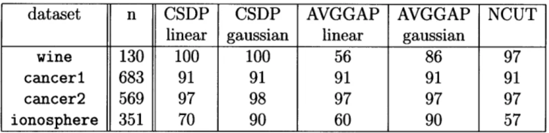
4.1 Clustering performance... . ...

52

Chapter 1

Introduction

We are currently building systems that produce more data at higher rates than ever before. With the advent of faster computers and a deluge of measurements from sensors, surveys, and gene arrays, building simple models to describe complex physical phenomena is a daunting challenge. Deriving simple models from data with principled tools that leverage a priori knowledge rather than expert tuning and annotation is of tantamount importance. Gaining intuitive understanding of these models and the modeling tools is equally important.

In this thesis, I will argue that if I can pose a modeling problem in terms of structured goals and constraints, then I can apply tools from convex optimization

to automatically generate algorithms to efficiently fit the best model to my data. In many regards, the main contribution is in problem posing. Not all problems can be posed as convex optimizations, but I will demonstrate through a variety of applications that this methodology is widely applicable and very powerful.

Recently, a great deal of interest has emerged around modeling complex systems with mathematical programming - the applied mathematics concerned with optimiz-ing cost functions under a set of constraints. Many modeloptimiz-ing, analysis, and design questions can be phrased as a series of goals and constraints. What is the shortest route from my house to work? What is the optimal strategy for managing con-gestion on the internet while maintaining user satisfaction [63]? How can an array of oscillators maximize their phase coherence [47]? Using the tools of mathematical

programming, a well-phrased problem statement alone can provide sufficient informa-tion to guarantee properties of system behavior, derive protocols for achieving optimal performance, and verify the convergence of the dynamics that solve the optimization. A special class of mathematical programs are the convex programs. Notable con-vex programs are the well-known problems of least-squares and linear programming for which very efficient algorithms exist. Building on these two examples, algorithms for convex optimization have matured rapidly in the last couple of decades. Today, the solution of convex programs is typically no more complicated than that of ma-trix inversion and the techniques have been applied in fields as diverse as automatic control, electronic circuit design, economics, estimation, statistical machine learning, and network design [15]. This puts the burden on the applied mathematician to either phrase a problem in a convex form or to recognize when this is not possible in an efficient manner.

Of course, not all problems can be phrased as convex optimizations. There are well-known classes of problems believed to be intractable independent of the applied solution technique. However, convex techniques have produced extremely good ap-proximations to many known hard problems. Such apap-proximations, called relaxations, provide guaranteed error bounds to intractable problems. Beginning with the work of Goemans and Williamson on approximating the NP-HARD problems MAX-CUT and MAX-2-SAT [37] in combinatorial optimization, an industry of approximating intractable problems to high tolerance has developed [31, 50, 52]. Whereas heuristic searches like genetic algorithms and simulated annealing provided no insight into the values they would output, the convex methods produce guaranteed error margins.

Inspired by these relaxations, this thesis will develop tools that exploit convexity to build approximate data-driven models incorporating expert a priori knowledge. My approach is cost function driven. By summarizing the modeling problem as a set of goals and constraints, I will systematically produce a convex representation of the problem of tractable size and an algorithm in the new representation which approximates the original formulation.

1.1

Contributions and Organization

In Chapter 2, I will provide a brief review of the mathematical foundations upon which this thesis rests. Beginning with an overview of convexity, I will summarize the theory of convex relaxations and Lagrangian duality, and I will discuss the connections with function learning on Reproducing Kernel Hilbert Spaces (RKHS), a powerful functional representation where the optimal mappings are sums of functions centered around each data point.

In Chapter 3, I will present a powerful cost function that can be applied to a vast array of data-driven modeling problems and can be optimized in a principled way. By augmenting the simple problem of fitting the best function in an RKHS to a set of data with a set of priors, I will produce a very general and powerful cost function for modeling with priors. This optimization seeks to jointly find the best model relating data to attributes, the labels of the unlabelled data, and the best space of functions to represent the relationship. The optimization will be convex in all of these arguments. In particular, I will present several novel results about learning kernel functions. I will provide a general formulation of the learning algorithms that may be solved with semidefinite programming. I will derive solutions to learning the width of Gaussian kernels. Finally, I will show how to search for the best polynomial kernel using semidefinite programming.

In Chapter 4, the first prior on the output will be presented. By restricting the desired outputs to be binary labels, a family of optimization problems for segmenta-tion, clustering, and transductive classification can be derived. I will show that even though the prior is so simple, all of the resulting optimizations are NP-HARD and no efficient algorithm to solve them exactly can be expected. In turn, I will present approximation algorithms using semidefinite programming. These semidefinite pro-grams may be prohibitively slow for very large numbers of examples, so I will also present an additional family of relaxations that reduce to eigenvalue problems. These eigenvalue problems recover the well-known Spectral Clustering algorithms. This function learning interpretation provides insight into when and how such algorithms

fail as well as how they can be corrected.

In Chapter 5, I describe a dynamics prior that results in a family of semi-supervised regression algorithms that learn mappings between time series. These algorithms are applied to tracking, where a time series of observations from sensors is transformed to a time series describing the pose of a target. Instead of defining and implementing such transformations for each tracking task separately, the algo-rithms learn memoryless transformations of time series from a few example input-output mappings. The learning procedure is fast and lends itself to a solution by least-squares or by the solution of an eigenvalue problem. I discuss the relationships with nonlinear system identification and manifold learning techniques. The utility of the dynamics prior is demonstrated on the tasks of tracking RFID tags from signal strength measurements, recovering the pose of rigid objects, deformable bodies, and articulated bodies from video sequences. For such tasks, these new algorithms re-quire significantly fewer examples compared to fully-supervised regression algorithms or semi-supervised learning algorithms that do not take the dynamics of the output time series into account.

Finally, in Chapter 6, I consider the problem of learning constraints satisfied by data. I show how to learn a space of functions that is constant on the data set and suggest how to select a maximal set of constraints. I show how this algorithm can learn descriptions of data sets that are not parsable by existing manifold learning algorithms. In particular, I show that this new algorithm can learn manifolds that are not diffeomorphic to Euclidean space.

1.2

Notation

This section serves as a glossary for the mathematical symbols used in the text. R denotes the real numbers and Z denotes the integers.

Vectors will be denoted by bold face lower case letters. Matrices will be denoted by bold face capital letters or capital Greek letters. The components of vectors and matrices will be denoted by subscripted non-bold letters. For example, the component

of the matrix A in the ith row and

jth

column is denoted Aj.

The transpose of a matrix A will be denoted by AT. The inverse of A is denoted A-1. When A is not necessarily invertible, the pseudoinverse of A is denoted by At.

1d denotes the d x d identity matrix. If its dimension is implied by the context,

then the subscript will be dropped. The vector of all ones is denoted 1. x > 0 means that each component of x is nonnegative.

An n x n matrix A is positive semidefinite if xTAx > 0 for all x

C

R4. Given two positive semidefinite n x n matrices A and B, A >- B means A - B is positive semidefinite. In particular, if A is positive semidefinite then we may write A >- 0.

The "-" relationship is a partial ordering on the semidefinite cone.

If x is an n-dimensional vector, diag x denotes the diagonal matrix with x on its diagonal. If, on the other hand A is an n x n matrix, diag(A) denotes the vector comprised of the diagonal elements of A. For example

diag = ,

(LX2 ) 0 X2

diag a1 1 a12 [all

(

a21 a22 a22

Let M be a matrix partitioned as

A B

M =

B T C

The Schur complement of A in M is defined to be

(MIA) = C - BTAtB

and the Schur complement of C in M is

The pseudoinverses are replaced by inverses when A or C are invertible. Some useful facts on Schur complements are presented in Appendix A.

The expected value of the random variable x will be written as E[x]. If there is confusion about the probability distribution, the expected value with respect to the distribution p will be denoted E,[x].

Chapter 2

Mathematical Background

2.1

Basics of Convexity

Beginning with Karmakar's famed interior point algorithm for linear programming [53], rapid advances in algorithms for efficiently operating with convex bodies have ren-dered convex programs generally no harder to solve than least-squares problems. Once a goal is phrased as a convex set of constraints and costs, it can usually be solved efficiently using a standard set of algorithms. Furthermore, a growing body of work in formulating problems in a convex framework shows a wide applicability across fields. This brief section will provide an overview of the features of convexity that make it such an attractive modeling tool. There are three objects which can be convex: sets, functions, and programs. I will describe what convexity means for each of these in turn.

2.1.1

Convex Sets

A set Q in Euclidean space is convex if it contains all line segments between all points.

For every x, and x2 in Q and every t between 0 and 1, the point (1 - t)x1 + tx2 is in

Q. Figure 2-1 shows two convex sets and one nonconvex set. Many familiar spaces

are convex. For example, the interior of a square or a disk are both convex subsets of the plane. There are other more abstract convex sets that commonly arise in

Convex

Non-convex

Figure 2-1: Left and Middle: Two convex sets. In each set a line segment is drawn between two points in the set and this line never leaves the set. Right: A nonconvex set. Two points are shown which cannot be connected by a straight line that doesn't leave the set.

mathematical modeling such as the set of possible covariance matrices of a random process. On the other hand, sets which are not convex abound as well. Neither the set of integers (try, for example, x1 = 1, x2 = 2, and t = 0.5) nor the set of invertible matrices are convex, and much of the art of convex analysis lies in recognizing when a set is convex.

An important tool for recognizing convex sets is a dictionary of operations that preserve convexity. For example, if 1,. . , £2m are convex, then their intersection (~=

₁

Q is convex. If Q is convex then any affine transformation of Q, {Ax+blx E Q} is convex. Furthermore, the premimage of an affine mapping is also convex. That is, if Q is convex, then so is {xIAx + b E l}.

2.1.2

Convex Functions

The epigraph of a function

f

: D --+ R is the set

epi(f) = {(x, y) : x E D y ;> f(x)} (2.1)

A convex function is a real-valued function whose epigraph is convex. That is, if the

set of all points lying above the value of the function is convex, then the function is convex (see Figure 2-2). Any linear function is convex as are quadratic forms arising I

from matrices with positive eigenvalues. Indeed, a quadratic form f(x) = xTQx

with Q = QT is convex if and only if Q >- 0. To see this, note that Q > 0 implies Q = AT A for some A. Then

x TQx = xTAT Ax = ||AxJ|2 (2.2)

and thus if (x1, yi) and (x2, y2) are in epi(f) and t E [0, 1,],

f(tx1 + (1 - t)x2) = ||A(tx1

+

(1 - t)x2)|

2

<

t||Ax

1

|

2 + (1

-

t)I|Ax

2

||

2 (2.3)

= tf(x1) + (1 - t)f(x2)

< tyi + (1 - t)y₂

proving that (tx1 + (1 - t)x2, ty1 + (1 - t)y2) E epif. Conversely, if Q is not positive semidefinite, let v be a norm 1 eigenvector corresponding to eigenvalue A < 0. Then (-v, A) and (v, A) are in epi(Q), but (0, A) is not, so

f is not convex.

As a consequence of (2.3),when the domain of

f is

R",

f is convex if and only if

f(txi + (1 - t)x2) tf(x1) + (1 - t)f(x2) . (2.4)

Many other simple functions are not convex including the trigonometric functions sine, cosine, and tangent and most polynomial expressions. An important feature of convex functions is their lack of local minima: if two points minimize a convex function locally, then both points achieve the same function value as do all the points along the line segment connecting them. This is one of the crucial features which makes the minimization of convex functions feasible.

Just as was the case with convex sets, there are a variety of operations that preserve the convexity of functions. For instance, if f(x) is convex then f(Ax + b)

is convex. If fi,... ,

f,

are convex, then so is a1fi + -.- + af, for any non-negative

scalars aj.

Convex Non-convex

Figure 2-2: Left: A convex function. One can readily check that the area above the blue curve contains all line segments between all points. Right: The red segment demonstrates

that the region above the graph is not convex.

family of convex functions f,,(x) with a in an index set I, fm(x) = supa fa(x) is a convex function. This can be verified by observing

epi(f) = {(x, y) : x E D y 2 fm(x)}

= {(x, y) : x E D y > sup

fa(x)}

a _(2.5)

= {(x, y) : x E D y > fa(x)Va E I}

=naeI{(x, y) : X ED y 2 fa(x)}

which is an intersection of convex sets and must be convex. Two immediate corollaries are that if fi, . . .,

f,

are convex, then maxi f2(x) is convex and, if for all y, f(x, y) is

convex in x, then sup, f(x, y) is convex. It is worth noting that

f

does not need to be convex in both x and y for this to hold.

For differentiable functions that map R" to R, convexity may be checked by inspecting derivatives. If

f

is differentiable,

f

is convex if and only if f(y) f(x) + Vf(x)T(y - x) for all y. If

f

is twice differentiable

f

is convex if and only if

V2f is positive semidefinite.

2.1.3

Convex Optimization

We will denote optimization problems

minimize f(x) _(2.6)

subject to x E Q by the short hand

min f(x) _(2.7)

s.t. x E Q

A convex program or convex optimization seeks to find the minimum of a convex

function

f

on a convex set Q. As was the case with convex functions, all local minima of convex optimizations are global minima. Remarkably, if testing membership in the

Q and evaluating

f

can both be performed efficiently, then the minimizer of such a problem can be found efficiently [39]. The most ubiquitous convex program is the least-squares problem which seeks the minimum norm solution to a system of linear equations. In this case

f

is a convex quadratic function and Q is Euclidean space.

A fundamental property of convex sets is that they are the intersection of all

half-spaces which contain them. That is, if a point x does not lie in a convex set, then the Euclidean space can be divided into two halves, one half containing x and the other half containing the convex set. This property suggests that when trying to find an

Figure 2-3: The convex set is separated from the points not in the set by half-spaces. The bold dashed line separates the plane into two halves, one containing the point x and the other containing the convex set.

optimal point in a convex set, one could also search over the set of half-spaces which contain the set (see Figure 2-3). Applying this reasoning to optimization, consider the optimization, called primal problem,

minimize f(x) _(2.8)

subject to gj(x);0

j=1,...,J.

Here f, g1, 92, ... , gj are all functions. This is a typical presentation of an optimization

problem: the set Q is the set of all x for which gj (x) is nonpositive for all

j

= 1, ... , J.

In linear programming, both the

f and all of the g

3 are linear maps.

The Lagrangian for this problem is given by

J

L(X, p) = f(x) + E jgj(x) (2.9)

j=1

with p > 0. The pt are called Lagrange multipliers. In calculus, we searched for values of p by using Vt2(x, p) = 0. Here, note that solving the optimization is equivalent to solving

min max /(x, p) (2.10)

xp2

The Dual Problem is the resulting problem when the max and min are switched.

max minCL(x, p) (2.11)

p20 x

The dual program has many useful properties. First, note that it provides a lower bound of the primal problem. We can show this by appealing to the more general logical tautology

min maxC (x, p) > max minC (x, p) (2.12)

x p2 0 p20 x

Indeed, let f(x, y) be any function with two arguments. Then f (x, y) min. f(x, y). Taking the max with respect to y of both sides shows maxy f(x, y) maxy min, f(x, y).

Now take the min of the right hand side with respect to x to show that

min max

f(x,

y) > max min

f(x,

y). (2.13)

x y y x

The dual program is always concave. To see this, consider the dual function

J

q(p) = minC (x, p) = min

f(x)

+ E yjg (x) (2.14) j=1

Now, since minx(f(x) + g(x)) > (min.

f(x))

+ (minx g(x)), we have J

q(tpi1 + (1- t)pt2) = mint f(x) +Epigg(x)

j=1

(2.15)

+ (1 - t) f(x) + E 2 j(x) j=1

> tq(pi) + (1 - t)q(p2)

which shows that q is a concave function and hence the dual problem is a convex optimization.

There is a nice graphical interpretation of duality. The image is the set of all tuples of numbers {(f(x), g(x))} for all x. In the image, the optimal value is equal to the minimum crossing point on the y-axis

[12].

The dual program seeks to find the half-space which contains the image and which has the greatest intercept with the f(x) axis. As shown in Figure 2-4, the maximum of the dual program is always less than the minimum of the primal program.

Duality is a powerful and widely employed tool in applied mathematics for a number of reasons. First, the dual program is always convex even if the primal is not. Second, the number of variables in the dual is equal to the number of constraints in the primal which is often less than the number of variables in the primal program. Third, the maximum value achieved by the dual problem is often equal to the minimum of the primal. One such example when the primal and dual optima are equal is when

f

and all of the gj are convex functions and there is a point x for which gj (x) is strictly

f(x) g(x) (p*,1) optimum f(x*) f(x*) (9*,1) (J4, 1)

Figure 2-4: The set of possible pairs of g(x) and f(x) are shown as the blue region. Left: Any hyperplane which has normal (p, _{1) intersects the y-axis at the point f(x*) + pTg(x*)} where x* minimizes C(x, p) with respect to x. Middle: A hyperplane whose y intercept is equal to the minimum of f(x) on the feasible set. The dual optimal value is equal to that of the primal Right: No hyperplane can achieve the primal optimal value. The discrepancy between the primal and dual optima is called a duality gap. The dual optimum value is always a lower bound for the primal.

negative for all

j.

_{Finally, if the primal program is not convex or not strictly feasible,} it is often possible to bound the duality gap between the primal and the dual optimal values. Estimating the duality gap is often difficult and, in many cases, this gap is infinite. However, for many practical problems, several researchers have discovered that one can meticulously bound the duality gap and produce sub-optimal solutions to the primal problems whose cost is only a constant fraction away from optimality. This is the study of convex relaxations.

2.2

Convex Relaxations

It is well known that finding the best integer solution to a linear program is NP-HARD. Many of the most successful and popular techniques for dealing with these generally hard problems solve the linear program for the best real valued solution, ignoring the constraint to the set of integers. One gets a lower bound on the optimum, and techniques such as branch and cut or branch and bound can be implemented. This is the most famous example of a convex relaxation. Indeed, this relaxation is well motivated by Lagrangian duality as the program obtained by dropping the integrality I

constraint has the same dual program as the primal integer program.

A series of surprising results have been developed over the last ten years using quadratic programming, rather than linear programming, to approach combinatorial problems. The general nonconvex quadratic program is also NP-HARD, and many hard combinatorial problems are naturally expressed as quadratic programs. For ex-ample, the requirement that the variable x takes on values 0 or 1 can be expressed by the quadratic constraint x2

= x. The dual program of a general nonconvex quadratic

program is a semidefinite program. Such optimizations can be solved efficiently using interior point methods [99] among other possible convex optimization techniques. For many structured quadratic constraints, one can actually estimate the worst case dual-ity gap. Moreover, for many problems of interest, there exists a randomized algorithm that produces a vector whose cost is within a constant factor 'y < 1 of the optimal primal value. A randomized algorithm which satisfies such an inequality is called a -/-approximation. There are several examples of hard problems in combinatorial op-timization where 'y is greater than 1/2. Indeed, for the famed MAX-CUT relaxation of Goemans and Williamson, y < 0.878 [37]. This is a great achievement considering that the existence of a polynomial time approximation to MAX-CUT with -y > 0.95 would imply P = NP, an equality which the majority of researchers in theoretical

computer science think is highly unlikely [43].

In this section I will summarize these techniques providing a unified presentation of the duality structure of nonconvex quadratic programs and how these duals can be used to provide bounds on combinatorial optimization problems. In Section 2.2.1, we will show that the Lagrangian dual of the general nonconvex quadratically constrained quadratic program is a semidefinite program. In Section 2.2.2 we will study how to bound the duality gap and to produce primal feasible points with near optimal cost.

2.2.1

Nonconvex Quadratically Constrained Quadratic

Pro-gramming

Let us begin with the general nonconvex quadratically constrained quadratic program min xTAox

+

2b Tx + CO

T 0 (2.16)

s.t. xTAix+2bTx+ci < 0 i=1,...,K

with x E R'. This problem is again NP-HARD (a recurring theme). It is, of course, well known that this problem is solvable efficiently when the Ai are positive semidef-inite, but in the situation where they are not, we have to rely on more sophisticated techniques for estimating the optimum.

Let's now examine the structure of the Lagrangian dual problem. First, we make a variable substitution to get the equivalent optimization

min yTQOy

s.t. yTQiy O i=1,...,K (2.17)

y2

where y is an n + 1 dimensional vector and ci bT Qi =(2.18)

bi Ai

We can think of y as the original decision variable x with a 1 stacked on top. The optimal value of Problem (2.17) is the same as (2.16). Any optimal solution of (2.16) can be turned into a minimizer for (2.17) by setting x = [1, x]. Since

yTQy = (-y)TQ(-y), any optimal solution for (2.17) can be turned into an optimal

solution for (2.16) by choosing the solution with yo = 1.

reformulated problem is then

(2.19)

L(y, , t) = yTQ(p, t)y + t

K

Q(A, t) = Qo + E piQi - t0 0 (2.20)

Minimizing with respect to y, we obtain negative infinity if Q(p, t) has any negative eigenvalues. In turn, we find that the dual function is given by

q(p,t) = _t

-oo0

Q(p, t) > 0

otherwise

and hence the dual problem is

max t

s.t. Qo + E= 1 piQi - t 00 >- 0

p > 0

(2.21)

(2.22)

This optimization is called a semidefinite program as the search is over the cone of positive semidefinte matrices. The dual can be solved efficiently using interior point

methods [99] among other possible convex optimization techniques.

Note that we don't worsen the dual bound by introducing the ancillary variable

yo. To see this, observe that we can break the dual program apart as follows

max minCL(y, p, t) = max max min min L(y, Y, t) p,t y y t yO yi,...,yn

For now, ignore the y maximization and consider the optimization y T

max min min YO

S x x

(2.23)

(2.24)

Performing the minimization with respect to x, we either get negative infinity or, if where

YO _{+ t(1 - y2)}

the matrix is positive semidefinite, we get the Schur complement of the quadratic form

maxminy6(-b T

Q-b

+ c - t) + t

t yo (2.25)

By inspection, the saddle point of this optimization is given when

t=-bTQ--b+ c

(2.26)

yo= 1

but that means

. .~nyo]T- - -max minmnO_{t Y}

(2.27)

That is, the dual values with or without the additional variable yo are the same. It is instructive to now compute the dual of the dual. A straightforward application of semidefinite programming duality yields the semidefinite program

min Tr(QoZ)

Tr(QZ) <0 i = 1,...,K (2.28)

Zoo = 1

Z

>_

0.

We can show that this relaxation can be derived by dropping refractory nonconvex constraints from the original primal program. This is similar to the relaxations of integer programming that utilize the linear program obtained by relaxing the inte-grality constraint. In the quadratic case, the constraint that we drop is a constraint on the rank of the matrix Z. To see this, first observe that we have the identity

yTQy = Tr(QyyT) (2.29)

c b T YO _{+ t(1 - Yo2}

.. _ -J - - __ _

1 c b T 1

and we can prove a simple

Proposition 2.2.1 Z = yy' for some y E R' if and only if Z is positive semidefinite

and has rank 1.

Proof If Z is positive semidefinite, we can diagonalize Z = VDVT where V is

orthogonal and D is diagonal. Without loss of generality, rank(Z) = 1 implies that D has d₁u > 0 and zeros elsewhere. Then if vi is the first column of V,

Z = divivT = ( diivi)(VdLvi)T (2.30)

Setting y =

v

ydjjv completes the proof. The converse is immediate. 0

Using this proposition, we can reformulate the original quadtratic program (2.17) as min Tr(QoZ)

Tr(QjZ)

<0

i = 1,...,IK Zoo = 1 (2.31) Z >- 0 rank(Z) = 1

The rank constraint is not convex, so a natural convex relaxation would be to drop it. Lo and behold, the resulting optimization is the semidefinite program (2.28).

Unlike the case of integer programming, for structured Qk we can actually

es-timate the worst case duality gap for this relaxation. In special cases, by solving problem (2.28), we can find a real number 'y < 1 and use a randomized algorithm to produce a vector y which is feasible for the optimization (2.17) such that

E[yTQoy] >

(2.32)

yT*Qoy*

-where y* is the optimum solution of the nonconvex problem. A randomized algorithm

will describe a particular application of this technique to combinatorial optimization.

2.2.2

Applications in Combinatorial Optimization

Consider the special nonconvex quadratic program

min x T Ax (2.33)

xE{-1,1} A

Where A is an arbitrary symmetric n x n matrix. This problem is inherently com-binatorial, and not surprisingly, is NP-HARD. We can write this as an nonconvex quadratically constrained quadratic program using the following extended represen-tation

min xTAx

(2.34)

The transformation of a set constraint into an algebraic constraint turns out to be the crucial idea. Indeed, there is no apparent duality structure to (2.33) as the only constraint is integrality. Once we have constraints, we can follow our nose and construct the dual program of (2.34)

min Ai

(2.35)

s.t. A+diag(A1,. . ., A) t 0

and we can use semidefinite programming duality again to find a relaxation for (2.33) min Tr AZ

s.t. diag(Z) = 1 (2.36)

Z > 0

This particular relaxation has been studied extensively in the literature, and led to a major breakthrough when Goemans and Williamson showed how to use it for

approximating the maximum cut in a graph. Before we proceed, let us quickly review some terminology from graph theory.

Let G = (V, E) be a graph and let w : E -- R be an arbitrary function. A

cut in the graph is a partition of the vertices into two disjoint sets V1, V2 such that

V1 U V2 = V. Let F(V) denote the set of edges which have exactly one node in V1.

By this definition F(V) = F(V2). The weight of the cut is defined the be

(2.37)

w(F) = E w(f)

fEF

Consider the optimization

MC(G,w) = max w(F(U)) s.t. U c V

(2.38)

If the weight function such that w(e) = 1 for all e E E, we denote the optimum solution as MC(G). This optimization is called MAX-CUT and is another of the classic optimization problems which are provably NP-HARD.

We can transform the optimization into an integer quadratic program by deriving the equivalent optimization problem

max 1 E w,,(1 - xUxV)

(UV)EE

s.t. x E {-1, 1}IV"I

(2.39)

The equivalence can be seen as follows: for every set U C V, let x" denote the

incidence vector of U in V and set x(U) = 2Xu - 1. Then if u E U, and v c U,

xux, = 1 and hence the edge between them is not counted. On the other hand if

u E U and v

g

U, xuxv = -1. It follows that j(1 - x-x,) = 1, and the edge between them is counted with weight wuv.

of G. The Laplacian is the |VI x |VI matrix defined by

-r ,

(u,v)

E

E

LU ZVAd(v) w,' u = V (2.40)

0

otherwise

where Adj(v) is the set of vertices adjacent to v. It is readily seen that (2.39) is equivalent to

max -xT Lx (2.41)

xE{-i,1}Ivi 4

Now we can apply the techniques developed in Section 2.2.1 to the max cut problem to yield the relaxation

1 max - Tr LZ

4

s.t. diag(Z) = 1 (2.42)

z >- 0

As noted before, we can solve this relaxation using standard algorithms for semidefi-nite programming.

Thus far we have not addressed the issue of the duality gap at all. We only know that (2.42) is an bound on the maximum cut in the graph. The breakthrough occurs in the algorithm providing a cut, that is, a primal feasible point, from the optimal solution of the relaxation. Consider the following algorithm:

(i) solve (2.42) to yield a matrix Z

(ii) sample a y from a normal distribution with mean 0 and covariance Z (iii) return x = sign(y)

if we define sign(0) = 1, x will always be a vector with l's and -1's and hence is primal feasible. As promised, we can characterize the expected quality of it's cut.

Theorem 2.2.2 (Goemans-Williamson) The algorithm of Goemans and Williamson produces a cut such that

IE[cut]_E~u]>

(2.43) MC(G) ~

with -y > 0.87856.

The proof relies on two lemmas, the first just a bit of calculus

Lemma 2.2.3 For -1 < t < 1, - arccos(t) > -yI(1 - t) with y > 0.87856

The proof of this can be found in [37], or can be immediately observed by plotting arccos.

The second lemma involves the statistics of the random variable x called a probit distribution. Determining the exact probability of drawing a particular x is practically infeasible to write down in closed form [46], and even approximating the probability would require an intensive Markov Chain Monte Carlo method (see for example [91]). Yet, if we only desire second order information, the situation is considerably better. Lemma 2.2.4 If y is drawn randomly from a Gaussian with zero mean and

covari-ance Z

1

Pr[sign(yi) 5 sign(yj)] = - arccos(Zig) (2.44)

7r

Proof Let n =

IVI

and let ei, 1 < i < n denote the standard basis for R". We have

Pr[sign(yi)

$

sign(yj)] = 2 Pr[yi > 0, yj < 0]

= 2 Pr[e y > 0, eTy < 0] (2.45) = 2Pr[vTw > 0, vTw < 0]

where w is drawn from a Gaussian distribution with zero mean and covariance I and vi = Z1_/2_{ei, v2 = Z}1_/2_{ej. Note that since Z has ones on the diagonal, the vectors vi}

and v2 lie on the unit sphere S

C

R n. Hence, the last probability is the ratio of the volume of the space

{x

E S" : vTx > 0, vTx < 0} to that of Sn. This is the ratio of

the angle between vi and v2to 27r. Thus we have

Pr[sign(yi)

#

sign(y)] = ₂arccos(vlV2)

1 27r (2.46)

= - arccos(Zi)

which completes the proof. U

We can now proceed to prove the quality of the Goemans-Williamson relaxation. Proof [of Theorem 2.2.2] For any edge e

c

E, let 6 denote the indicator function for e in the cut. Then the expected value of a cut is

E[cut] = weE[6e] w = Wi Pr[sign(yi)

#

sign(yj)]

eEE i<j 1 E wij arcos(Zij) 7r (2.47) i<j 1 -y Tr(LZ) 4 So we have E[cut] > 7 Tr(LZ) 7MC(G). M

Remarkably, this technique of sampling from a probit distribution generalizes to a wide class of problems in combinatorial optimization. Notably, Nesterov generalized the results of Goemans and Williamson to a 2/7r-approximation for the more general optimization problem [68]

max xTAx (2.48)

xE{-1,1}n

with A >- 0. His technique rephrases (2.48) as a nonlinear semidefinite program, and then uses the partial order on the semidefinite cone to yield his bound.

Let arcsin(M) denote the component-wise arcsin of the matrix M.

Theorem 2.2.5 (Nesterov)

2

max xT Ax = - max Tr(A arcsin(Z)) (2.49)