Cooperate to compete : composable planning and inference in multi-agent reinforcement learning

Cooperate to Compete:

Composable Planning and Inference in Multi-Agent

Reinforcement Learning

by

Michael M. Shum

Submitted to the Department of Electrical Engineering and Computer

Science

in partial fulfillment of the requirements for the degree of

Master of Engineering in Computer Science and Engineering

at the

MASSACHUSETTS INSTITUTE OF TECHNOLOGY

June 2018

c

○ Massachusetts Institute of Technology 2018. All rights reserved.

Author . . . .

Department of Electrical Engineering and Computer Science

May 25, 2018

Certified by . . . .

Joshua B. Tenenbaum

Professor

Thesis Supervisor

Certified by . . . .

Max Kleiman-Weiner

Graduate Student

Thesis Supervisor

Accepted by . . . .

Katrina LaCurts

Chairman, Department Committee on Graduate Theses

Cooperate to Compete:

Composable Planning and Inference in Multi-Agent

Reinforcement Learning

by

Michael M. Shum

Submitted to the Department of Electrical Engineering and Computer Science on May 25, 2018, in partial fulfillment of the

requirements for the degree of

Master of Engineering in Computer Science and Engineering

Abstract

Cooperation within a competitive social situation is a essential part of human social life. This requires knowledge of teams and goals as well as an ability to infer the intentions of both teammates and opponents from sparse and noisy observations of their behavior. We describe a formal generative model that composes individual planning programs into rich and variable teams. This model constructs optimal coordinated team plans and uses these plans as part of a Bayesian inference of collaborators and adversaries of varying intelligence. We study these models in two environments: a complex continuous Atari game Warlords and a grid-world stochastic game, and compare our model with human behavior.

Thesis Supervisor: Joshua B. Tenenbaum Title: Professor

Thesis Supervisor: Max Kleiman-Weiner Title: Graduate Student

Acknowledgments

This thesis describes work done with Max Kleiman-Weiner and Josh Tenenbaum. I would like to thank them for all their mentorship and advice. In particular, Max has inspired my interest in research and guided me while still allowing me to make this project my own. For the brainstorming sessions, life advice, and technical guidance, I am extremely grateful.

I would also like to thank Patrick Winston and Katrina LaCurts for the opportu-nities to TA 6.034 and 6.033.

Last but not least, I would like to thank my family for their continual belief, support, and advice.

Contents

1 Introduction 10

1.1 Motivation . . . 10

1.2 Reinforcement Learning . . . 12

1.2.1 Markov Decision Processes . . . 12

1.2.2 Reinforcement Learning Algorithms . . . 13

1.2.3 Issues in Reinforcement Learning . . . 14

1.3 End-to-End Construction of Teams . . . 15

2 Warlords and Deep Reinforcement Learning 16 2.1 Deep Reinforcement Learning . . . 17

2.1.1 DQN Architecture . . . 18

2.2 Warlords Game Construction . . . 19

2.3 Training a Single Agent . . . 20

2.3.1 Modified Reward Structures . . . 21

2.4 Moving On . . . 25

3 Social Planning and Stochastic Games 26 3.1 Naturalistic Games . . . 26 3.2 Model . . . 27 3.2.1 Social Planning . . . 27 3.2.2 Joint Planning . . . 28 3.2.3 Individual Planning . . . 30 3.3 Behavioral Experiments . . . 30

3.3.1 Human Ranges of K-Levels . . . 31

3.4 Sequences of Observations . . . 35

4 Composable Team Structures and Inference 36 4.1 Operations and Base Atoms . . . 36

4.2 Composing Multi-Agent Teams . . . 38

4.2.1 Team Theory of Mind . . . 39

4.2.2 Inference of Teams . . . 40

4.3 Real-Time Dynamic Programming . . . 41

4.4 Stag Hunt . . . 42 4.5 Results . . . 43 4.5.1 Speed . . . 43 4.5.2 Inference of Teams . . . 44 5 Discussion 45 5.1 Selecting Teammates . . . 45 5.2 Scalability in Planning . . . 46 5.3 Partial Observability . . . 47

5.4 Self-Play-Trained Level 0 Agents . . . 47

5.5 Conclusion . . . 47

List of Figures

2-1 Starting configuration for the Atari game Warlords. . . 17

2-2 A frame from Warlords gameplay. . . 17

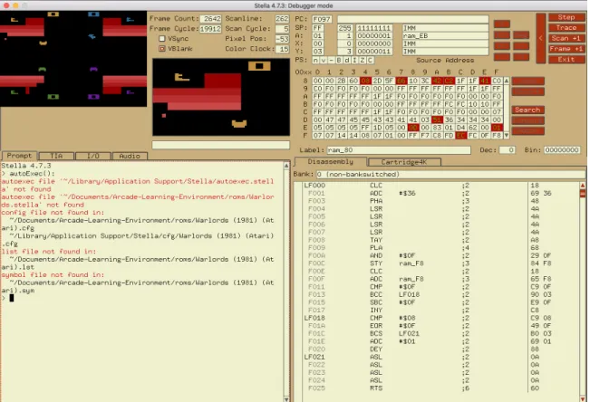
2-3 Debugger mode in the Stella emulator. . . 20

2-4 Rewards per episode for Warlords with Bricks configuration. . . 22

2-5 Rewards per episode for Warlords with Defense configuration. . . 23

2-6 Rewards per episode for Warlords with Double configuration. . . 23

2-7 Rewards per episode for Warlords with Breakout configuration. . . 24

3-1 Example of a naturalistic game. . . 27

3-2 Regression model of human data against individual and joint model predictions. The individual model had R=0.856 and the joint model had R=0.897. . . 32

3-3 Heatmaps showing likelihood of movements for players A, B, C in various games and starting states. For each player and spatial location, both the averaged human and model predictions for the next move for each of the three agents is shown as a red probability heatmap. Each column shows a different arrangement of the three players. . . 33

3-4 Level k=2 planning for a 3x3 game. . . 34

4-1 Examples of composing policies to model different team structures with agents of variable sophistication. . . 39

4-2 Starting state for a Stag Hunt. . . 43

List of Tables

A.1 Number of states for each environment. . . 49 A.2 Average times in seconds for VI vs LRTDP vs BRTDP for an agent

with K=1. . . 49 A.3 Average times in seconds for VI vs LRTDP vs BRTDP for an agent

with K=2. . . 49 A.4 Average number of Bellman updates made for VI vs LRTDP vs BRTDP

for an agent with K=1. . . 50 A.5 Average number of Bellman updates made for VI vs LRTDP vs BRTDP

Chapter 1

Introduction

1.1

Motivation

Finding the right balance between cooperation and competition is a fundamental challenge for any agent in a multi-agent world. This balance is typically studied in two-player games such as prisoner’s dilemma, where each player must choose whether to pay a cost in order to make the group better off (cooperate) or selfishly optimize only one’s own welfare (compete). Humans are especially adept at finding cooperative solutions and maintaining the balance [1]: we are more cooperative, have larger social groups, and are more flexible than any other animal species. A celebrated result is that reciprocity, cooperating with those who cooperate and competing with those who choose to compete, can sustain cooperation [2, 3, 4, 5]. While reciprocal games like prisoner’s dilemma are typically studied in a matrix-form game, this result holds true in richer environments where cooperative intentions must be inferred from sparse observations of action in order to be understood and reciprocated [6].

However when the number of agents increases beyond a two player dyadic in-teraction, balancing cooperation and competition takes on a qualitatively different character. Unlike with two players where the decision is binary (to cooperate or compete with the other person), in situations with three or more players individuals must reason about which agents they should cooperate with and which to compete against. In environments with limited resources and conflicting incentives, cooperation

itself requires competition: agents have to cooperate in order to compete.

In domains with structured teams known in advance such as sports or business, "rules" are clear and the structure of the teams are essentially written into the reward function of the environment. Yet within a team, agents might not necessarily play "as a team". When helping out the group is costly, individuals might optimize for a more selfish reward e.g. showing off in a sports contest or only contributing to a group project when they will get credit. This is readily seen when calling someone a "team player" – one is truly considering the objective of the team, not just their own individual reward. Since both allies and adversaries are of variable sophistication and ability, it is still a challenge to develop and execute a detailed joint plan of action while inferring plans of teammates even when teams are known [7].

While there has been recent success in two-player zero-sum games such as Go and Poker [8, 9, 10] adding additional players makes these players lose their zero-sum characteristics and the algorithms designed to play these games (often trained through self-play) are no longer guaranteed to play optimally. Adding an additional player creates multiple equilibria so even a zero-sum game with three of more players suffers from the same multiple equilibrium problems that mixed-incentive games have. Thus little work on self-play will naively generalize to these richer scenarios. An algorithm which plans only through self-play will find itself unable to adapt to situations outside of the equilibria it converged to. Consider even a simple case of three-player poker. If two of the three players collude against the third then they will be able to exploit the third player over time even though the game is itself is zero-sum.

Outside of highly organized games, team structure is not known in advance. Consider the case of a child learning cultural norms: the structure of cooperation (i.e., who is friendly and who is not) might be set but unknown to the learner. Teams can also fluidly change, as in children’s games like tag where "it" is passed from player to player. Humans naturally infer the new team structures, i.e., who is the chaser and who is fleeing just from a few sparse samples of behavior [11]. In other cases, the teams form dynamically in response to the demands of a particular situation. This occurs across many scales from rival groups of hunters collectively chasing prey [12, 13] to

sovereign nations deciding who they should ally with. In order to understand common sense social concepts that people use regularly such as friendship and ally we need machines that can understand these terms in the same ways we do.

Our contribution is a representation and formalism for understanding and planning with teams of other agents. We take an approach inspired by models of human planning. [14, 15]. Humans solve these problems using a rich cognitive tool-kit that includes the ability to model other agents [16, 17] to decide what they should do in any particular situation.

1.2

Reinforcement Learning

In order for computational agents to construct plans, they use an area of machine learning called reinforcement learning. Reinforcement learning enables an agent to find an optimal behavioral strategy while receiving feedback from only the environment. The agent receives information about the state of the environment, can take actions which may affect the state of the environment, and finally receives a reward or punishment signal that gives feedback about the action taken. Ultimately, the goal of reinforcement learning is finding a policy that maximizes the long-term reward. Much of this background is from Sutton and Barto’s Introduction to Reinforcement Learning [18].

1.2.1

Markov Decision Processes

Reinforcement learning environments are formally described using Markov decision processes. A Markov decision process is defined by

∙ states 𝑆

∙ actions 𝐴,

∙ rewards 𝑅𝑎

∙ transition probabilities 𝑃 , where the probability that action a is taken in state 𝑠 to state 𝑠′ is 𝑃𝑎

𝑠,𝑠′.

An agent interacts with its environment in discrete steps, so at any time 𝑡, the Markov decision process is in state 𝑠𝑡. At that time 𝑡, the agent chooses an action

𝑎𝑡 from the set of actions 𝐴, which transitions the environment from state 𝑠𝑡 to the

successor state 𝑠𝑡+1 with probability 𝑃𝑠𝑎𝑡𝑡,𝑠𝑡+1. The agent then receives a reward 𝑟𝑡+1

from that action.

Reinforcement learning then primarily involves solving a Markov decision process to find what actions are best in what states. This mapping of states to actions is called a policy.

1.2.2

Reinforcement Learning Algorithms

One method for solving reinforcement learning problems is value iteration. It aims to estimate the expected return of being in a given state and is defined via a value function 𝑉 (𝑠). Using a given policy 𝜋, 𝑉𝜋(𝑠) is the expected reward when starting from state 𝑠.

𝑉𝜋_{(𝑠) = E[𝑅|𝑠, 𝜋]}

Value iteration uses the Bellman equation (1.1) as an update rule.

𝑉𝜋_{(𝑠) = E} [︃ _∞ ∑︁ 𝑡=0 𝛾𝑡𝑅(𝑠𝑡) ]︃ = max 𝑎 ∑︁ 𝑠′_∈𝑆 𝑃_𝑠,𝑠𝑎 ′(𝑅𝑎_𝑠,𝑠′ + 𝛾𝑉𝜋(𝑠′)) (1.1)

A Bellman backup is defined by updating 𝑉 (𝑠) for all states in 𝑠. With infinite backups, convergence to the optimal value function 𝑉* is guaranteed and is referred to as full value iteration. However in practice, full value iteration terminates once the value function changes by less than an 𝜖 amount in a backup.

Using the value function 𝑉𝜋_{, a Quality function 𝑄}𝜋_{(𝑠, 𝑎) then maps states and}

𝑄𝜋(𝑠, 𝑎) =∑︁

𝑠′_∈𝑆

𝑃_𝑠,𝑠𝑎 ′(𝑅𝑎_𝑠,𝑠′ + 𝛾𝑉𝜋(𝑠′))

Clearly when using the optimal value function 𝑉*, this equation provides a set of optimal Q values 𝑄*(𝑠, 𝑎) with which an optimal policy can be retrieved by choosing an action greedily at each state: argmax_𝑎𝑄*(𝑠, 𝑎).

Value iteration is a dynamic programming method that "bootstraps", meaning it uses existing estimates of 𝑉 and 𝑄 to upate future estimates. Temporal-difference (TD) methods like Q-learning augment dynamic programming methods by sampling from the environment. As an example, an on-policy method called SARSA updates its V and Q functions in 1.2 and 1.3. The on-policy component here refers to the fact that updates to 𝑄 are made by using transitions generated by the existing policy 𝑄𝜋_.

𝑉 (𝑠𝑡) ← 𝑉 (𝑠𝑡) + 𝛼[𝑟𝑡+1+ 𝛾𝑉 (𝑠𝑡+1) − 𝑉 (𝑠𝑡)] (1.2)

𝑄(𝑠𝑡, 𝑎𝑡) ← 𝑄(𝑠𝑡, 𝑎𝑡) + 𝛼[𝑟𝑡+1+ 𝛾𝑄(𝑠𝑡+1, 𝑎𝑡+1) − 𝑄(𝑠𝑡, 𝑎𝑡)] (1.3)

An off-policy variant of TD methods is Q-learning, where transitions may be generated by a different policy than the one being followed. An example is shown in 1.4.

𝑄(𝑠𝑡, 𝑎𝑡) ← 𝑄(𝑠𝑡, 𝑎𝑡) + 𝛼[𝑟𝑡+1+ 𝛾 max

𝑎 𝑄(𝑠𝑡+1, 𝑎) − 𝑄(𝑠𝑡, 𝑎𝑡)] (1.4)

1.2.3

Issues in Reinforcement Learning

Regardless of the method used, reinforcement learning faces two specific challenges that continue to plague it.

∙ The only learning signal an agent receives is the reward. This means agents must interact through trial and error with the environment to discover the reward. ∙ Actions taken by an agent may not lead to immediate rewards, leading to an

credit assignment problem.

1.3

End-to-End Construction of Teams

In games with fluid team structures, an individual looking to best plan has to follow a sequence of steps.

1. Identify team structures: which could be my teammates and what are the other teams?

2. Select a team: which are my best options for teammates?

3. Inferring teammates: what other agents are demonstrating cooperation? 4. Planning: what is my team’s best course of action; what is my best action?

Chapter two describes our initial exploration of planning in the Atari game Warlords. This includes a background of deep reinforcement learning.

Chapter three explores social planning where teams and goals are known and introduces the concepts of joint and individual planning.

Chapter four defines a formal grammar with which individuals and observers can construct possible team structures and infer in an environment where teams are unknown.

Chapter 2

Warlords and Deep Reinforcement

Learning

We first attempted to build models that could play cooperatively in an Atari game, Warlords. Warlords is a battle between 4 players, where the objective is to destroy the other three castles while protecting your own castle with a moving shield. The castles are the L-shaped blocks contained within the red bricks as seen in Figure 2-1. A single red ball ricochets around the screen and bounce off walls and shields, but upon colliding with bricks destroys them. An example of this gameplay is shown in Figure 2-2. By moving the shield in the path of the ball, the ball ricochets in the opposite angle it approached with. However, if the player holds 𝑠𝑝𝑎𝑐𝑒𝑏𝑎𝑟 while the ball hits the shield, the player "catches" the ball and can move in order to shoot at high speed in their specified direction. Since the ball can move at higher speeds than shields, we expected that interesting coalitions may form where multiple players can team up to "pass" the ball and quickly attack another player.

Atari games are particularly challenging to learn due to their complex continuous nature. Given the recent success in using deep reinforcement learning to play Atari games [19, 20], we aimed to first train an agent to learn an optimal individual policy and then extend it to learn optimal team policies as well as infer teammates.

Figure 2-1: Starting configuration for the Atari game Warlords.

Figure 2-2: A frame from Warlords gameplay.

2.1

Deep Reinforcement Learning

Atari games are easily understood by humans, but the complex state space represented by mere pixels make them difficult for artificial intelligence agents to learn. The sheer number of states a game can be in make it difficult for a computer to brute-force a strategy, even for a single-player game with a clear goal like Pong or Breakout. In 2013 DeepMind introduced Deep Q Networks (DQN) [19], a method that uses a neural network as a nonlinear function approximator to compute Q values. This allowed it to scale to problems that were intractable due to high-dimensional state and action spaces, and it achieved super-human performance.

We recall that Q functions assign values for each state-action pair. With large problems, one method to work around the intractability of fully solving for Q is to learn an approximate value function 𝑄𝜋_{(𝑠, 𝑎; 𝜃) ≈ 𝑄}𝜋_{(𝑠, 𝑎). A standard approach is}

to use a linear function approximation, where 𝑄𝜋(𝑠, 𝑎; 𝜃) = 𝜃⊤𝜑(𝑠, 𝑎), such that 𝜃 is a vector of weights and 𝜑(𝑠, 𝑎) is a feature of the state action pair. However, DQN’s innovation to kickstart deep reinforcement learning was the ability to use nonlinear

function approximation methods, specifically neural networks, to approximate the Q function.

2.1.1

DQN Architecture

Atari games have high-dimensional visual inputs; DQN preprocesses the screens to size 84x84, converts to grayscale with 256 gray levels, and only uses 4 screen images. Some quick math reveals this to be 25684*84*4 _{states, an intractable number of states to solve}

with value iteration. Especially since a vast majority of these pixel combinations are never reached, we need a way to condense our screen into manageable features. By using convolutional neural networks (CNNs) as a component of reinforcement learning agents, agents learn directly from the visual inputs. DQN represents the Q-function with a neural network that takes in four game screens as state, and outputs Q-values for all possible actions from that state. This neural network has three convolutional layers and two fully connected layers.

Convolutional layers allow the network to learn powerful internal representations [21]. Convolutional networks apply a single filter in all sections of an image, condensing them into features. This allows it to generalize observations, like "a red pixel near a red brick is bad", instead of needing to see every combination of the ball hitting every pixel of brick. This alone doesn’t encode movement, so DQN uses four consecutive game screens to embed each object’s direction. The filter sizes in each convolutional layer are also set to sizes that are roughly the sizes of typical agents in Atari games, in order for the network to detect objects. After the convolutional layers create features, the fully connected layers decide a non-linear function from these features that finally outputs values for each action.

Neural networks are trained by optimizing a loss function, and DQN uses a squared error loss of the temporal difference error from before.

𝐿 = 1

2[𝑟 + 𝛾 max𝑎′ 𝑄(𝑠𝑡+1, 𝑎𝑡+1) − 𝑄(𝑠𝑡, 𝑎𝑡)]

2

backpropaga-tion.

Nonlinear function approximators were not effectively utilized until DQN since they frequently would diverge when updates were not based on on trajectories of the Markov chain [22]. In order to solve this, DQN uses experience replay and target networks. Experience replay stores transitions of (𝑠𝑡, 𝑎𝑡, 𝑠𝑡+1, 𝑟𝑡+1) in a buffer, and

takes batches of these transitions at a time to update the network. This reduces the number of interactions and breaks the temporal correlations that RL algorithms can be affected by. Target networks can be thought of as the off-policy concept from Q-learning, where the policy network uses a fixed target network that is updated after a fixed number of steps. This allows the TD error to be compared to a weight matrix that isn’t constantly fluctuating.

2.2

Warlords Game Construction

In order to train agents to play Atari games, researches use an interface called the Arcade Learning Environment (ALE) [23]. The ALE is a platform that provides an interface to Atari game environments built on top of Stella, an Atari 2600 emulator. For common Atari games like Breakout and Pong, the ALE comes with ROMs as well as functions that identify action sets and return rewards taking steps.

Warlords is not included in the ALE. We used Stella to identify the RAM locations of bricks and castles. At every step of the game, the step method checks these locations for changes to specific values to identify bricks or hearts destroyed. We used the Stella debugger (Figure 2-3) to step through frames of the game and find which RAM locations pertained to bricks and hearts. We found that locations 0x8F through 0x(F (except for 0x95 and 0x96) held hex values that related to the yellow player’s two-brick sets being destroyed. Starting from 0xFF, these would decrease based on the order of bricks being destroyed. Additionally location 0xEE held an indicator to which castles had been destroyed, since an increase of 0x8F represented the yellow castle being destroyed.

Figure 2-3: Debugger mode in the Stella emulator.

2.3

Training a Single Agent

Once we identified how to modify the reward structure and relevant actions, we leverage OpenAI’s Baselines algorithms [24] and Gym interface [25] to the ALE to train our agents. Gym allows us to modify interfaces to environments (like setting the mode of a game). Baselines includes open-source implementations of deep reinforcement learning algorithms like DQN and variants like A3C [26], A2C, and ACKTR [27]. The 2013 DQN paper used 1 million frames, while the 2015 paper used 50 million frames to train its algorithm before testing. Baselines operates using timesteps, which each contain 4 frames. The default setting is 10 million timesteps (40 million frames), and we generally used this as our cutoff. We found it took roughly 24 hours to train for 10 million timesteps.

We first attempted to train a single agent playing against all others to learn an intelligent policy. Since the goal is to destroy other player’s bricks while staying alive, the game is similar in structure to Breakout and Pong, both of which DQN achieved

super-human performance on. As a result we expect this to be a trivial first step, given the correct reward structure.

Breakout and Pong were trained only given the score of the game: Breakout receives one point for every brick destroyed and loses a point for every life lost, while Pong receives one point for every score and loses one for every point scored against. However Warlords only provides a point once all enemy castles have been destroyed, and no points are lost for one’s own castle being destroyed. As a result, even after training the agent was unable to learn an intelligent policy. We gathered this was due to the reward being much more sparse than those from Breakout and Pong.

2.3.1

Modified Reward Structures

Knowing this, we attempted to modify the reward structures as well as different modes of the game. While the underlying structure of the game remains the same, there are 23 different modes that modify number of players, shield behavior, and ball speed. The number of players can be between 1-4, and involves a Doubles mode that allows a single agent to control two players against another single two-player joint agent. Shield behavior can remove the catch functionality, making the ball ricochet only when colliding with the shield. Ball speed can be modified between fast and slow speeds. The default behavior is 4 players with catching and fast ball speed.

We also removed the catch functionality in the hopes of reducing the action space. The expectation was to first observe intelligent behavior in the form of the paddle deflecting the ball.

We first modified reward to be +100 for destroying other castles and -100 for one’s own castle being destroyed in the hopes that an amplified reward structure could lead to enough credit attribution. We aimed to impart as little structure to the algorithm as possible, as humans are only given the score as well, but this was as ineffective as +1/-1.

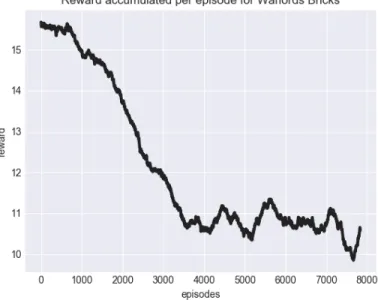
We then modified reward to be +1 for other bricks being destroyed and -1 for one’s own bricks being destroyed, in addition to +10 for a castle being destroyed and -10 for one’s own castle being destroyed. This also did not lead to intelligent behavior

Figure 2-4: Rewards per episode for Warlords with Bricks configuration.

in 10 million timesteps. A learning curve is shown in Figure 2-4, where reward is shown over episodes (a full play of the game until termination). While the plot shows positive reward per episode, this is due to the fact that agents can earn points even when losing a brick due to the ricochet. Additionally due to the three other players and corners, agents earn points without taking intelligent actions and as a result are unable to attribute the correct actions to the actual rewards earned. Even without any other agents taking actions, the ball ricochets from one corner of bricks to another, earning our agent points.

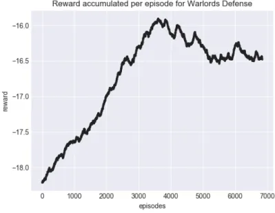
In order to remove this ability to be rewarded arbitrarily, we modified the reward to only be -1 for one’s own bricks being destroyed. We hoped this would lead to a defensive strategy of deflecting the ball. The learning curves are shown in Figure 2-5. While it appears that the agents are beginning to lose fewer points, in fact agents are attempting to lose as quickly as possible since they have no incentive to stay alive.

Hoping to reduce the parameters, we switched to a Doubles configuration. This causes our agent to control both yellow and green shields. We hoped that with one agent controlling an entire half, fewer bricks being hit would be attributed incorrectly. A plot is shown in Figure 2-6. In this case, we observe that reward increases, indicating

Figure 2-5: Rewards per episode for Warlords with Defense configuration.

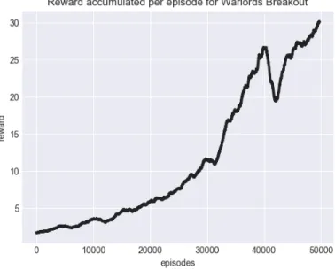
Figure 2-7: Rewards per episode for Warlords with Breakout configuration.

agents stay alive for longer but upon visual observation very rarely did agents make movements to block the ball. We hypothesized that with longer training, it might be possible to train an intelligently acting agent. However, given that it took 10 million steps to train an intelligently acting agent while it only took 3 million to train an intelligent agent in Breakout and Pong, this did not seem like the most optimal route.

We finally modified the game-ending condition to be when any of one’s own bricks were destroyed, hoping to replicate Breakout’s success. It was only with this change that we observed behavior consistent with expectation – the shield moves to defend the ball. Similar to early versions of trained agents in Breakout, the motions were jerky rapid movements, where the shield would shoot across the screen at the last second to block the ball. While the ball was far away, unlike human or built-in game AI behavior, the shield would not track the trajectory of the ball. A plot is shown in Figure 2-7. We imagine this may be remedied if the shield’s movement speed were limited.

2.4

Moving On

We originally intended to have our agents control multiple players in the game. The expectation was that we could explore creating agents with shared reward functions that still planned individually, as well as an agent that planned jointly. We hoped to observe mis-coordination between individually planning agents. Once we had agents with these behaviors, we hoped to have a version online that allowed human beings to play with our agents that would allow us to observe our model’s ability to collaborate with agents outside our own models. Further, we had intended to explore the difference between DQN, A3C, ACKTR, and Schema Models; would one of these be more effective or amenable to being augmented to cooperate?

This exploration comprised 4 months of work. We observed that only semi-intelligent behavior emerges after significantly modifying the gameplay structure and training for a long period of time. Even with an ability to deflect the ball, we saw none of the team dynamics that catching and passing the ball might indicate. Given that our goal was to explore how models may construct teams, infer teammates, and plan optimally, we decided to forsake this domain and scale down to something more manageable.

Chapter 3

Social Planning and Stochastic

Games

Even when teams and goals are known, coordinating team plans is a challenge. Teammates can be of varying sophistication, and their behavior may be noisy. Here we explore how agents can construct optimal team plans and coordinate those plans. We use the idea of strategic best response, a concept commonly used in behavioral game theory [15, 14] and recently extended to reinforcement learning [6, 12] known as cognitive hierarchy, level-K, and iterative best response depending on specific implementation (see [15] for a review and comparison of these subtly different models). The general idea is to perform a finite number of iterative best responses to a base model which is not strategic. By only considering a finite number of iterations we prevent an infinite regress as well as capture some intuitive constraints on bounded thinking.

3.1

Naturalistic Games

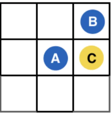
While traditionally social behavior consists of game-theoretic investigations in matrix-form games, social decisions are much more naturally explored in naturalistic spatial environments like video games. Simple grids similar to those introduced in [28], like Figure 3-1, are a useful way to represent a variety of games since people intuitively

Figure 3-1: Example of a naturalistic game.

orient themselves spatially and so form complex plans almost without any other knowledge.

In this chapter, all games explored are a single round of Tag between one team of two players and one team of one player. Each player controls the movement of one of the colored circles throughout the course of the game. On each turn players choose to move their circles into adjacent squares (not diagonal) or stay in the same spot. All players select an action during the same turn and all positions are updated simultaneously. If there are collisions between teammates they remain in the same place, while any collision between opposing players (moving into the same square, moving into each other’s squares, or one player moving into a stationary player’s square) counts as a tag and the end of the game.

After every turn the team that is "It" collectively loses 1 point while the team being chased gains 1 point. Once the chasing team catches a single player the "It" team receives 10 points, the team being chased loses 10 points, and the game ends. As a result the game is zero sum with respect to teams.

3.2

Model

3.2.1

Social Planning

We build a model of strategic planning that can form joint intentions assuming equally intelligent teammates, or varied lower levels of intelligence for other players. Agents

know of the existence of teammates and share the rewards with them. At every step, agents select their action with a plan formulated under a presumption of each other player’s intelligence. This model-based learning generalizes well with multiple players as well as in new environments.

This work builds on classical formalisms of intention and joint planning from AI literature [29, 30] in addition to traditional reinforcement learning techniques [18]. Models in previous work do not handle uncertainty in a probabilistic way and so struggle with predictions about behavior.

Following the notation of De Cote and Littman [31], we construct stochastic games representing different childrens’ games. A three-player stochastic game is represented as ⟨𝑆, 𝑠0, 𝐴1, 𝐴2, 𝐴3, 𝑇, 𝑈1, 𝑈2, 𝑈3, 𝛾⟩ where 𝑆 is the set of all possible

states with 𝑠0 ∈ 𝑆 as the starting state. If assuming equal intelligence, each agent

chooses from a set of actions 𝐴𝑎𝑏 constituting the joint actions of the team. Otherwise,

an agent selects an action from its set of actions 𝐴𝑎. A state transition function

𝑇 (𝑠, 𝑎1, 𝑎2, 𝑎3) = 𝑃 (𝑠′|𝑠, 𝑎1, 𝑎2, 𝑎3) represents likelihoods of moving to new states given

states and individual actions from agents. Reward for an individual player 𝑖 is given as 𝑈𝑖. Additionally 0 ≤ 𝛾𝑔𝑎𝑚𝑒 ≤ 1 is a discount rate of reward.

We define agents as attempting to maximize their joint utility, assuming other agents are doing the same. To represent this game-theoretic best response, we use the level-K formalism used in behavioral game theory with regards to the policies used by both teams [14, 32]. In a two-player game a level-K agent best responds to a level-(K-1) agent, which results in a level-0 agent. In our models, a level-0 agent is a randomly acting agent. This seems reasonable since the environment doesn’t have specified goals, only to survive.

3.2.2

Joint Planning

If agents assume their teammates are at the same level they are in, the optimal action comes from treating the team as a single-agent [33]. As a result, they can construct level-K rollouts to identify the best team-action before marginalizing the actions of their teammate to identify their individual best action.

Accordingly, a randomly moving level-0 agent for a team with players 𝑖 and 𝑗 would have equal probability for any legal joint action for both players.

𝑃 (𝑎𝑖𝑎𝑗|𝑠, 𝑘 = 0) = 𝜋𝑖0(𝑠) ∝ exp 𝛽𝑄0

𝑖(𝑠,𝑎𝑖𝑎𝑗)

𝑄0_𝑖(𝑠, 𝑎𝑖𝑎𝑗) = 0

With a level-0 agent defined, a level-k agent for players 𝑖 and 𝑗 on a team against player ℎ on an opposing team can be recursively constructed in terms of lower levels.

𝑃 (𝑎𝑖𝑎𝑗|𝑠, 𝑘) = 𝜋𝐺(𝑠, 𝑎𝑖𝑎𝑗) = exp𝛽𝑄 ( 𝑖𝑘)(𝑠,𝑎𝑖𝑎𝑗) 𝑄𝑘_𝑖(𝑠, 𝑎𝑖𝑎𝑗) = ∑︁ 𝑠′ 𝑃 (𝑠′|𝑠, 𝑎𝑖𝑎𝑗) (𝑈 (𝑠′, 𝑎𝑖𝑎𝑗, 𝑠) + 𝛾 max 𝑎′_𝑖𝑎′_𝑗 𝑄 𝑘 𝑖(𝑠 ′ , 𝑎′_𝑖𝑎′_𝑗) (3.1) 𝑃 (𝑠′|𝑠, 𝑎𝑖𝑎𝑗) = ∑︁ 𝑎ℎ 𝑃 (𝑠′|𝑠, 𝑎𝑖𝑎𝑗, 𝑎ℎ)𝑃 (𝑎ℎ|𝑠, 𝑘 = 𝑘 − 1)

Here, player ℎ is treated as part of the environment and so is described within 𝑃 (𝑠′|𝑠, 𝑎𝑖𝑎𝑗). The maximization operator allows the joint agent to build the

best-response to the level-(K-1) agent. Clearly this could be expanded to teams of any-sized 𝑛 players against teams of similarly any-sized 𝑚 players.

With a policy defined for the joint actions for a team via the underlying 𝑄𝑘_𝑖(𝑠, 𝑎𝑖𝑎𝑗),

a single agent 𝑖 on the team can marginalize out the actions of its teammate. 𝜋𝐺

𝑖 (𝑠, 𝑎𝑖) =

∑︀

𝑎𝑗𝜋

𝐺_{(𝑠, 𝑎}

𝑖𝑎𝑗) and similarly for player 𝑗. These individual policies contain intertwined

intentions that include an expectation for the teammate to reach certain states. This is a meshing of plans that is a key component of joint and shared intentionality [34, 35]. Crucially, agents here assume teammates are at the same level K they themselves are at.

3.2.3

Individual Planning

Agents can also assume teammates are at a lower level than the ones they themselves are in. Notably, reward is still earned if teammates achieve the goal. For this experiment, we assume all other agents are at level-(K-1).

A randomly moving level-0 agent then for player 𝑖 only includes actions 𝑎𝑖.

𝑃 (𝑎𝑖|𝑠, 𝑘 = 0) = 𝜋𝑖0(𝑠) ∝ exp 𝛽𝑄0

𝑖(𝑠,𝑎𝑖)

𝑄0_𝑖(𝑠, 𝑎𝑖) = 0

Thus, an agent 𝑖 doing individual planning at level-K with teammate 𝑗 and opponent 𝑘 constructs its policy with

𝑃 (𝑎𝑖|𝑠, 𝑘) = 𝜋(𝑠, 𝑎𝑖) = exp𝛽𝑄 ( 𝑖𝑘)(𝑠,𝑎𝑖) 𝑄𝑘_𝑖(𝑠, 𝑎𝑖) = ∑︁ 𝑠′ 𝑃 (𝑠′|𝑠, 𝑎𝑖)(𝑈 (𝑠′, 𝑎𝑖, 𝑎𝑗𝑠) + 𝛾 max 𝑎′ 𝑖 𝑄𝑘_𝑖(𝑠′, 𝑎′_𝑖)) 𝑃 (𝑠′|𝑠, 𝑎𝑖) = ∑︁ 𝑎𝑗,𝑎ℎ 𝑃 (𝑠′|𝑠, 𝑎𝑖𝑎𝑗, 𝑎ℎ)𝑃 (𝑎𝑗|𝑠, 𝑘 = 𝑘 − 1)𝑃 (𝑎ℎ|𝑠, 𝑘 = 𝑘 − 1)

The assumption that a teammate is one level lower is one that could be developed over time. In the future an optimal agent could infer the K-levels of other agents based on their actions over the course of the game and adjust to them. In our experiments, we utilized values of K-1 for both teammates and opponents and tested the self K to be either 1 or 2. This means agents expect all other players to be moving randomly, or best responds to an agent expecting everybody else to be moving randomly.

3.3

Behavioral Experiments

We constructed seven game states and asked 20 participants to pick where they would go in the next move as each player. Participants were given instructions that detailed the purpose of the game, goals of each player, scoring system, and dynamics

of the environment. After seeing the state, participants were asked to select one of 𝐿𝑒𝑓 𝑡, 𝑅𝑖𝑔ℎ𝑡, 𝑈 𝑝, 𝐷𝑜𝑤𝑛, 𝑆𝑡𝑎𝑦 as the next move for player 1, 2, and 3.

In comparing model predictions with human behavior, we tallied the count of each movement for each player for the state. We then created red heatmaps where each square’s color intensity is proportional to the ratio of the movement count to all movements – the more people that chose a movement the redder the square that would be moved to. We also visualized the softmax policies for each model, with the probability of moving to a square determining the redness of that square.

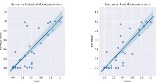
Figure 3-3 shows the decisions of one model with individual planning and one model with joint planning, compared to human decisions. The individual model assumes it is level K=1, which assumes all other players are K=0. The joint model operates assuming the team is level K=1 and the opponent is level K=0. Globally we observe that both models capture the human data well, almost fully capturing the range of human decisions and generally capturing the distribution across actions as well. For all models we used a relatively high softmax 𝛽 value of 7, as well as a 𝛾 discount rate of 0.9. We also plotted every human decision for each game against the model’s decisions in Figure 3-2 and found a correlation coefficient of 0.897 for the joint model and 0.856 for the individual model.

Between models, we note that the individual model is less likely to consider the space of other moves than the joint model. This is most evident for agent B, especially in columns 2 and 4. As a result the joint model captures the human data better. Since our current model only does value iteration and state sizes grow exponentially as the board becomes larger, it was difficult to compute level K=2 heatmaps for all starting states. However, when conducting the experiment the most interesting human behavior was in starting state 4 (column 4); we will describe it in more detail as well as explore heatmaps for level K=2 models.

3.3.1

Human Ranges of K-Levels

We identified that K=1 models did not accurately capture the human sentiment to move down for player 2 in state 2 and built a level K=2 model to see if it was more

Figure 3-2: Regression model of human data against individual and joint model predictions. The individual model had R=0.856 and the joint model had R=0.897.

accurate, shown in Figure 3-4.

For Player 1, both joint and individual models at level K=2 accurately captured the human intuition to move down or stay still. This intuitively makes sense since player 2 closes off the middle square.

Player 2 has the most diverse set of possibilities out of all squares shown. Human data shows participants equally preferred staying still, moving right, and moving down. Both level K=1 models strongly preferred moving right and slightly staying still, reflecting their understanding that player 3 moves randomly. However the level K=2 individual model roughly equally weight staying still and moving down and place no weight on moving right, and the joint model reflect the human beliefs thoroughly. This captures the other human responses shown previously, which expect that player 1 will move down and prevent player 3 from escaping by moving left. It appears that different participants considered player 3 to be at different intelligence levels. Interviewed after their selections, participants who elected to move down said they didn’t believe player 3 would be smart enough to move left. This would reflect a belief that player 3 is a level 1 agent.

Human data for Player 3 was almost entirely 𝐷𝑜𝑤𝑛, with only two participants selecting 𝐿𝑒𝑓 𝑡. Similar to Player 2 this reflected the fact that most humans were

Figure 3-3: Heatmaps showing likelihood of movements for players A, B, C in various games and starting states. For each player and spatial location, both the averaged human and model predictions for the next move for each of the three agents is shown as a red probability heatmap. Each column shows a different arrangement of the three

Figure 3-4: Level k=2 planning for a 3x3 game.

thinking at a Level 2. However some participants selected 𝐿𝑒𝑓 𝑡, signifying that they were at Level 3. This would hope for Player 2 to move down, allowing Player 3 to escape through the middle.

It appears that humans operate as either level 2 and level 3 models. This decision may either reflect their ability to imagine steps ahead, a bias to underestimate the opponents, or a lack of time. Participants expressed an interest in playing out more moves in order to feel out other players’ intentions. Some participants also said the more states they saw the less thought they tended to put into them due to the high initial cost of imagining scenarios. For future work it would be useful to explore the play of individuals over an entire game. This would allow us to more concretely identify what level individuals were playing at, as well as allow them to be more invested and accurate in their moves. The immediate feedback would be helpful in engaging participants.

We notice that humans never assumed opponents were moving randomly or that they were static. Most people projected what their possible range of actions were as opponents and did a best-response to that. However, humans interviewed said that they couldn’t trust teammates to operate at the same level they were. This lack of trust in teammates was due to the zero-shot nature of the experiment, where humans weren’t given any information about the other players. Upon observing moves, we hypothesize that humans are likely to gain trust in a teammate if they follow the joint

policy at their own level-K. Notably a player might not gain trust in their teammate if the teammate’s policy is a level-(K+1) since it might not be understood.

We note that a level-K policy only operates well in response to a level-(K-1) policy. Using Figure 3-4’s state again, a level K=2 player two might move down with 60% probability which could allow a level-0 random player the opening to escape into the middle square. This is a key result from Wako Yoshida’s Game Theory of Mind [12].

3.4

Sequences of Observations

Even with knowledge of teammates and goals, individuals typically observe more than one still image before making plans. One significant inference is the intelligence of one’s teammates (thus far referred to as K level). Certainly, agents could be augmented to dynamically infer partner’s K-levels and adapt their policies over the course of the game instead of fixing parameters throughout. Additionally, given different games a random level 0 agent may not be the most representative action; it could be static or have its own limited intentions. An interesting experiment would be to first compare human’s inferences of K levels of all other players after observation of a few actions, and then given the true K levels compare the plans humans construct with those of our model.

Chapter 4

Composable Team Structures and

Inference

Once we know how to plan optimally given teams and goals, we need a way to construct potential team structures and infer which of these team structures is the most likely representation of the environment. We do so by augmenting the previous concept of strategic best response (level K) with a model of joint intentionality. To explore our models’ abilities to infer teammates and construct plans, we extend a stag hunt from 2 hunters to 3 hunters.

4.1

Operations and Base Atoms

In behavioral game theory [15, 36], level-K is referred to as cognitive hierarchy, as well as iterative best response. Here, we define an agent finding a policy given a lower-level model by best responding as BR (best response). This recursive step continues until it reaches a non-strategic base atom, also known a level-0 policy. Redefining 3.1 for clarity, a randomly acting level-0 agent A has policy 𝜋0_𝐴:

𝜋_𝐴0(𝑠) = 𝑃 (𝑎𝐴|𝑠, 𝑘 = 0) ∝ exp𝛽𝑄

0 𝐴(𝑠,𝑎𝐴)

A level-K model for a single agent B is then defined recursively: 𝜋_𝐵𝑘(𝑠, 𝑎𝐵) = 𝑃 (𝑎𝐵|𝑠, 𝑘) ∝ exp𝛽𝑄 𝑘 𝐵(𝑠,𝑎𝐵) 𝑄𝑘_𝐵(𝑠, 𝑎𝐵) = ∑︁ 𝑠′ 𝑃 (𝑠′|𝑠, 𝑎𝐵)(𝑅(𝑠′, 𝑎𝐵, 𝑠) + 𝛾 max 𝑎′_𝐵 𝑄𝑘_𝐵(𝑠′, 𝑎′_𝐵) 𝑃 (𝑠′|𝑠, 𝑎𝐵) = ∑︁ 𝑎−𝐵 𝑃 (𝑠′|𝑠, 𝑎𝐵, 𝑎−𝐵)𝑃 (𝑎−𝐵|𝑠, 𝑘 = 𝑘 − 1)

Since the other agents are treated as a knowable stochastic part of the environment, the transition probability 𝑃 (𝑠′|𝑠, 𝑎𝐵) encapsulates the dynamics of the other agents,

denoted by 𝑃 (𝑎−𝐵|𝑠, 𝑘 = 𝑘 − 1), where −𝐵 is a shorthand to refer to all other agents.

Due to the maximization operator, a level K agent implements a best response policy to a level K-1 agent.

While the Level-K model can capture strategic thinking (i.e., how to best respond to other agents), by itself it is not sufficient to generate cooperative behavior. Thus we also consider a second planning procedure that aims to approximate the results of centralized planning in a decentralized way. In short, the procedure combines the individual agents into a centralized “team-agent” that has joint control of all the agents that are included in the team.

Although the objective function of the planner is centralized, the actual planning process and execution of the plan itself are assumed to be decentralized. Thus each agent carries out this planning process with information that is common to the team. We define JP (joint planning) which takes a stochastic game 𝐺𝐴,𝐵 with agents 𝐴 and 𝐵 as input, merges the remaining players into a “team-agent” which can control the joint action space and the reward of all players into a shared reward, plans optimally, and decomposes into individual policies.

After replacing agent C, merging the action spaces for agents A and B (𝑎𝐴, 𝑎𝐵)

from 𝐺𝐴,𝐵 into a joint action space 𝑎𝐴𝐵 within a new game 𝐺𝐴𝐵 creates a single-agent

MDP. As a result the joint agent can run the same planning algorithms from before to find a joint policy.

𝑄𝐴𝐵(𝑠, 𝑎𝐴𝐵) = ∑︁ 𝑠′ 𝑃 (𝑠′|𝑠, 𝑎𝐴𝐵)(𝑅𝐴𝐵(𝑠′, 𝑎𝐴𝐵, 𝑠) + 𝛾 max 𝑎′ 𝐴𝐵 𝑄𝐴𝐵(𝑠′, 𝑎′𝐴𝐵)) 𝜋𝐴𝐵(𝑠, 𝑎𝐴𝐵) = 𝑃 (𝑎𝐴𝐵|𝑠) ∝ exp𝛽𝑄𝐴𝐵(𝑠,𝑎𝐴𝐵)

In the same way as BR, the transition function of 𝐺𝐴𝐵, 𝑃 (𝑠′|𝑠, 𝑎𝐴𝐵) embeds the

policies of other agents (here, agent C). Since a policy is probabilistic, each agent plays its role in the team by marginalizing out the actions of all the other agents. As an example for agent A:

𝜋𝐴(𝑠, 𝑎𝐴) =

∑︁

𝑎𝐵

𝜋𝐴𝐵(𝑠, 𝑎𝐴𝐵)

4.2

Composing Multi-Agent Teams

The core of our contribution is that using these simple components we can create highly complex team plans where agents vary in their cooperative orientation as well as in their sophistication. Our approach is that under the right model of other agents, multi-agent planning can be described as the flexible composition of single agent planning algorithms with a model of the environment.

Even with just three players (A, B, C) there are a combinatorial number of possible team structures, each of which could have varying intelligence levels and methods of construction.

1. [ABC] (all players cooperating together) 2. [AB] vs [C] (A and B on a team against C) 3. [AC] vs [B],

4. [A] vs [BC],

5. [A] vs [B] vs [C] (all players competing against each other).

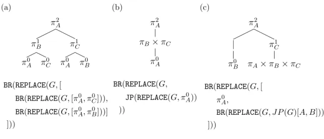
Figure 4-1 shows how atomic level-0 policies for individual agents can be composed together to create policies for individual agents (with BR), as well as for teams of cooperative agents (using JP). Above are tree structures that visualize the hierarchy of

(a) 𝜋2 𝐴 𝜋1 𝐵 𝜋0 𝐴 𝜋0𝐶 𝜋1 𝐶 𝜋0 𝐴 𝜋𝐵0 BR(REPLACE(𝐺, [ BR(REPLACE(𝐺, [𝜋0_𝐴, 𝜋_𝐶0])), BR(REPLACE(𝐺, [𝜋0_𝐴, 𝜋_𝐵0]))] ])) (b) 𝜋2 𝐴 𝜋𝐵× 𝜋𝐶 𝜋0 𝐴 BR(REPLACE(𝐺, JP(REPLACE(𝐺, 𝜋0_𝐴)) )) (c) 𝜋2 𝐴 | 𝜋0 𝐵 𝜋1 𝐶 𝜋𝐴× 𝜋𝐵× 𝜋𝐶 BR(REPLACE(𝐺, [ 𝜋_𝐴0, BR(REPLACE(𝐺, 𝐽 𝑃 (𝐺)[𝐴, 𝐵])) ]))

Figure 4-1: Examples of composing policies to model different team structures with agents of variable sophistication.

how mental models are constructed, and below are the corresponding grammars. For a level K=2 agent A, tree (b) shows a composition assuming team structure [A] vs [BC], while trees (a) and (c) demonstrate two possible compositions of team structure [A] vs [B] vs [C]. We explore how these composition are constructed in the next section.

4.2.1

Team Theory of Mind

With a representation that can generate possible team configurations we now describe how agents use trees like Figure 4-1 to construct plans. Given a game 𝐺 that includes all agents 𝐴, 𝐵, 𝐶 and their respective action spaces and reward functions, an individual agent A can first identify all team structures as above. It then recursively best responds as an individual agent with BR or as a joint agent with JP to other agents. It does so with a REPLACE operator that takes 𝐺 and a list of policies [𝜋𝐵, 𝜋𝐶, . . . ], and replaces

players in the game with their respective policies. Having replaced all other agents in the game with policies, the game becomes a single-player MDP that BR and JP can completely solve.

In order to construct the policies used in REPLACE, agents continue recursively replacing players in lower-level games until they reach base atoms of level-0 policies. With a given maximum K-level depth and team structure, agent A can construct all

possible trees using only BR, JP, and REPLACE operators.

As an example, tree A shows how a level K=2 agent A given team structure of [A] vs [B] vs [C] solves for its policy by best responding to what agents B and C will do. Agent A has to determine how agent B and agent C will make decisions – what team structures do agents B and C have in their minds? In tree A’s construction, agents B and C also assume a team structure of [A] vs [B] vs [C]. Since B and C are level-1 agents, their mental models of other agents are level-0, and those are base atoms at the leaves of the tree. We can rewrite the grammar under tree A in a bottom-up construction for clarity:

𝜋0_𝐴, 𝜋0_𝐵, 𝜋_𝐶0 ← 𝐵𝑎𝑠𝑒𝐴𝑡𝑜𝑚𝑠 𝜋_𝐵1 = BR(REPLACE(𝐺, [𝜋_𝐴0, 𝜋_𝐶0])) 𝜋_𝐶1 = BR(REPLACE(𝐺, [𝜋_𝐴0, 𝜋_𝐵0])) 𝜋_𝐴2 = BR(REPLACE(𝐺, [𝜋1_𝐵, 𝜋_𝐶1]))

Tree B shows an example of using JP where the same level K=2 agent A assumes a team structure of [A] vs [B+C]. Since agents B and C are on a team in A’s mind, agent A maintains a mental model of a level K=1 joint agent [B+C] that best responds to a level-0 agent [A]. Note that while a joint agent [B+C] has policy 𝜋1_𝐵𝐶, agent A best responds to a marginalized ([𝜋1

𝐵, 𝜋𝐶1]) and recomposed policy 𝜋𝐵1 × 𝜋1𝐶, since B and C

are not directly controlled by the same agent. Again rewriting the grammar under tree B in a bottom-up way:

𝜋_𝐴0 ← 𝐵𝑎𝑠𝑒𝐴𝑡𝑜𝑚 𝜋_𝐵1 × 𝜋1 𝐶 = JP(REPLACE(𝐺, 𝜋0𝐴)) 𝜋_𝐴2 = BR(REPLACE(𝐺, [𝜋1_𝐵× 𝜋1 𝐶]))

4.2.2

Inference of Teams

Our models can then use the policies computed after using Team Theory of Mind to make posterior updates of their beliefs of the team structures in their environment.

These updates are made after observing a single action taken by every player. Defining 𝑚 as the relevant team members from team structure 𝑇𝑚 (e.g. members [AB] from

team structure [AB] vs [C]), a posterior is the likelihood of taking action 𝑎𝑚 multiplied

by the prior 𝑃 (𝑇𝑚).

𝑃 (𝑇𝑚|𝑎𝑚, 𝑠) ∝ 𝑃 (𝑎𝑚|𝑇𝑚, 𝑠)𝑃 (𝑇𝑚)

By aggregating (normalized) likelihoods from all trees with the same team structure, we have our likelihood of this team structure. We can index into the policy at the root of each tree to retrieve the likelihood for each tree. Here, trees are symbolized as 𝑅, where there are 𝑖 trees with team structure 𝑇𝑚.

𝑃 (𝑎𝑚|𝑇𝑚, 𝑠) ∝

∑︁

𝑖

(𝜋𝑅𝑖[𝑠][𝑎𝑚])

4.3

Real-Time Dynamic Programming

Because the number of possible states is exponential in the number of agents, exactly computing the policies with full value iteration for anything but the simplest games is intractable. However, the assumption of approximately rational agency is a strong one – under almost any agent model most states are not reachable with any significant probability. In this section we apply tools for bounded planning that are highly suited to exploit this feature of multi-agent plans.

In principle any planning algorithm works depending on the problem – we could use value iteration or even deep RL. Here we take a more model based approach in using Real-Time Dynamic Programming (RTDP) [37] an algorithm with strong convergence guarantees [38, 39]. RTDP-based algorithms simulate the current greedy policy in order to sample trajectories through the state space, and perform Bellman backups only on states in those trajectories. We utilize two variants of RTDP called Labeled RTDP (LRTDP) and Bounded RTDP (BRTDP).

LRTDP identifies 𝜖-consistent states and marks them as solved. Once a state becomes 𝜖-consistent, future Bellman backups are guaranteed to not change 𝑉 (𝑠) or

the values of any descendants of s by more than 𝜖. This allows LRTDP to detect convergence and terminate trials early, especially if initialized with a good heuristic. BRTDP not only keeps track of the value function but also keeps a monotone upper bound 𝑉𝑢 on 𝑉 *, in addition to a lower bound. Performing a Bellman backup

to either bound thus results in a closer approximation to 𝑉 *, eventually converging on the optimal values. Maintaining upper and lower bounds allows BRTDP to evaluate a measure of uncertainty about the state’s value via the difference between bounds, and focuses its sampling on states where the value function is less understood (where the uncertainty is larger). By using these bounds BRTDP guarantees convergence without touching all reachable states.

We hypothesize that RTDP variants will perform well in this scheme because rational behavior is highly constrained. That is, in a multi-agent setting most states are extremely unlikely when other agents are assumed to be acting rationally. As a result, by sampling trajectories following a greedy policy we can avoid unnecessary computation in solving single-agent MDPs. In section 4.5.1 we validate this approach, even without heuristic values for either algorithm.

4.4

Stag Hunt

In game theory, a stag hunt is a game in which there are two Nash equilibria – one is risk dominant and one is payoff dominant. In the game, two individuals are on a hunt. Each individual can choose to hunt either a stag or a hare, without knowing what the other person’s choice. If both choose to hunt the stag they will catch it, but if one chooses the stag without the other he dies. Hunters can catch the hare without the other, but a hare is worth much less than a stag. The conflict between safety and cooperation lead to the game also being called a "coordination game" and "trust dilemma". Wako Yoshida extends this matrix-form game to a naturalistic game [12], and we extend her two-hunter game to 3 hunters. An example game is shown in Figure-4-2.

Figure 4-2: Starting state for a Stag Hunt.

catches a stag, they each receive 20 points, but if a single hunter is killed by a stag it loses 20 points. After each timestep, each hunter loses one point. Stags earn one point at every timestep they were alive, incentivizing them to stay alive as long as possible. After any hunter catches any hare or stag, or after any hunter is killed by a stag, the game ends. Both hunters and stags can only move in adjacent directions (up, down, left, right, no diagonals), or stay still.

4.5

Results

4.5.1

Speed

In order to compare LRTDP and BRTDP to full value iteration (VI), we initialized games with varying state spaces and numbers of agents. We then had one agent fully converge on a policy and timed how long the computation took for the three different algorithms. In cases where the computation took more than 1800 seconds, we stopped the calculation. We also tracked the number of Bellman updates made for all three algorithms. Each experiment was repeated 10 times and the numbers were averaged. Tables with this data can be found in Appendix A.

Figure 4-3: Inference of team structures over time for a 3rd party observer.

Both variants of RTDP vastly outperform VI in time and number of Bellman updates.

4.5.2

Inference of Teams

A 3rd party observer can also use the same formalism to infer the team structure of a game given a few observations of the environment. This inference is quite similar to the one performed by a single agent, but the likelihoods of actions are now multiplied across all teams within the team structure. That is, after observing a single action taken by every player, an observer could update a posterior of team structure 𝑇𝑚𝑛 by

multiplying the likelihood for team 𝑚 and likelihood for team 𝑛 with the prior 𝑃 (𝑇𝑚𝑛)

and normalizing. For a more concrete example, 𝑚 could be [A+B] and 𝑛 could be [C].

𝑃 (𝑇𝑚𝑛|𝑎, 𝑠) ∝ 𝑃 (𝑎𝑚|𝑇𝑚, 𝑠)𝑃 (𝑎𝑛|𝑇𝑛, 𝑠)𝑃 (𝑇𝑚𝑛)

In the same way as before, we can aggregate likelihoods from all trees with a given team structure to get individual likelihoods like 𝑃 (𝑎𝑚|𝑇𝑚). In Figure-4-3 we see an

Chapter 5

Discussion

While we achieved many of the steps we set out to – formulating team structures, inferring teammates, and coordinating optimal plans, we still lack a principled method of selecting teammates the way humans might. Additionally planning is still limited in the size of games and number of agents that can be modeled, our games assume full observability that real life doesn’t guarantee, and level 0 agents are always assumed to be random. Here, we explore how to remedy these issues.

5.1

Selecting Teammates

Agents have the ability to infer the most likely team structures, but in all experiments they begin with uniform priors over all team structures and select teammates purely based on the posterior of the most likely team. This is not representative of how humans form teams – people have underlying goals that drive them to form specific teams, and may have existing priors on how cooperative another agent might be. This manifests itself commonly in international relations: a long-standing concern is what motivates states to follow international norms [40], and with whom are they willing to come to terms with?

A simple augmentation to the model would be setting the probability of selecting a team structure by augmenting the posterior of the team after observation with a softmax of the V values at a state:

𝑃 (𝑇𝑚|𝑎𝑇𝑚, 𝑠) ∝ 𝑃 (𝑎𝑇𝑚|𝑇𝑚, 𝑠)𝑃 (𝑇𝑚)

𝑃 (𝑇𝑚) ∝ 𝑃 (𝑇𝑚|𝑎𝑇𝑚, 𝑠) exp

𝛽𝑉𝑇𝑚(𝑠)

This weighting incentivizes agents in early stages to demonstrate cooperation to teammates that lead to higher reward, but if the cooperative intent is consistently not reciprocated agents will still be able to infer and select a better team. Ideally this could lead to interesting propositions of teams as well as convergence on teams in different starting states and environments.

Further, instead of starting with a uniform prior agents could retain a posterior of cooperation with other agents across games. This might be based on demonstration of cooperative intent in previous games, but could also be influenced by norms of some kind. Individuals who may not be "team players" might seek to be the best player on their team – they may elect to only cooperate with others of equal or lower ability. Other interesting possibilities that appear in human behavior include players teaming up against a heavy favorite to overthrow them, or instead joining the favorite in order to be on a winning side.

5.2

Scalability in Planning

Even with the improvements made to planning with RTDP, we are still unable to scale to larger games. What if we want to evaluate the cooperative intent of huge groups? One approach taken is to model a large population as a mean field game (MFG), where the population is represented by their distribution over state space and each agent’s reward is a function of the population’s distribution as well as the total actions. By modeling agents as a distribution, MFGs are able to scale up to massive population sizes. Yang et al [41] have created a method for MFG inference by using MDP policy optimization, and show that a case of MFG can be reduced to a MDP whose optimal policy is equivalent to inference of the MFG model.

BRTDP, we initialize the upper and lower bounds to arbitrary values that guarantee being larger and smaller than the true 𝑉 *. However, with lower bounds convergence is much more rapid. Using deep reinforcement learning here may be a viable option, as we could utilize it to identify heuristic values that have tighter bounds.

5.3

Partial Observability

In addition to games with full observability, we could implement games with limited visibility. Agents next to blocked squares may be temporarily unable to view the locations of other players. These uncertainties could be included in the models by averaging expected locations of agents around swaths of area, or by modeling as a POMDP [42]. Further, new agents could be introduced to the game and known agents could be removed. This could lead to interesting configurations of how team structures are created and updated with new knowledge.

5.4

Self-Play-Trained Level 0 Agents

This approach is model-based. Since all actions are made by the individual, they could find the best responses themselves. Self-play has been shown to allow simulated AIs to discover physical skills without designing an environment for those mind [43], and to learn a strategy for Texas Hold’em that approached the performance of state-of-the-art methods [44]. We could use self-play to find priors for more accurate level-0 models. This could lead to more accurate inferences of teammates and team structures.

5.5

Conclusion

In fully-observable environments, we formalize a model that can identify team struc-tures, infer teammates, and coordinate optimal plans. Our models have an ability to reason about other group and individual agents’ intents and make predictions about their behaviors in order to best-respond. This ability to do inference is an extension

Appendix A

Tables

Table A.1: Number of states for each environment.

k1 small k1 medium k1 large k1 huge VI 4.62 72.627 591.722 None LRTDP 0.313 0.0711 0.509 0.514 BRTDP 0.353 0.091 0.477 0.485

Table A.2: Average times in seconds for VI vs LRTDP vs BRTDP for an agent with K=1.

k2 small k2 medium k2 large k2 huge VI 56.28 1919.457 None None LRTDP 29.947 19.274 3021.1 None BRTDP 20.543 0.989 9.014 168.405

Table A.3: Average times in seconds for VI vs LRTDP vs BRTDP for an agent with K=2.

k1 small k1 medium k1 large k1 huge VI 175824 2718848 20104866 None LRTDP 449.315 89.42 555.36 444.89 BRTDP 772.05 189.75 875.4 793.8

Table A.4: Average number of Bellman updates made for VI vs LRTDP vs BRTDP for an agent with K=1.

k2 small k2 medium k2 large k2 huge VI 3422080 109663101 None None LRTDP 71678.0 7780.57 None None BRTDP 87462.0 2190.15 14889.45 596266.9

Table A.5: Average number of Bellman updates made for VI vs LRTDP vs BRTDP for an agent with K=2.

Bibliography

[1] M. Tomasello, A natural history of human thinking. Harvard University Press, 2014.

[2] R. L. Trivers, “The evolution of reciprocal altruism,” Quarterly review of biology, pp. 35–57, 1971.

[3] L. Cosmides and J. Tooby, “Cognitive adaptations for social exchange,” The adapted mind: Evolutionary psychology and the generation of culture, vol. 163, pp. 163–228, 1992.

[4] R. Axelrod, The Evolution of Cooperation. Basic Books, 1985.

[5] M. A. Nowak, “Five rules for the evolution of cooperation,” Science, vol. 314, no. 5805, pp. 1560–1563, 2006.

[6] M. Kleiman-Weiner, M. K. Ho, J. L. Austerweil, M. L. Littman, and J. B. Tenenbaum, “Coordinate to cooperate or compete: abstract goals and joint intentions in social interaction,” in Proceedings of the 38th Annual Conference of the Cognitive Science Society, 2016.

[7] M. Babes, E. M. De Cote, and M. L. Littman, “Social reward shaping in the prisoner’s dilemma,” in Proceedings of the 7th international joint conference on Autonomous agents and multiagent systems-Volume 3. International Foundation for Autonomous Agents and Multiagent Systems, 2008, pp. 1389–1392.

[8] D. Silver, A. Huang, C. J. Maddison, A. Guez, L. Sifre, G. Van Den Driessche, J. Schrittwieser, I. Antonoglou, V. Panneershelvam, M. Lanctot et al., “Mastering the game of go with deep neural networks and tree search,” nature, vol. 529, no. 7587, pp. 484–489, 2016.

[9] D. Silver, J. Schrittwieser, K. Simonyan, I. Antonoglou, A. Huang, A. Guez, T. Hubert, L. Baker, M. Lai, A. Bolton et al., “Mastering the game of go without human knowledge,” Nature, vol. 550, no. 7676, p. 354, 2017.

[10] N. Brown and T. Sandholm, “Superhuman ai for heads-up no-limit poker: Libratus beats top professionals,” Science, p. eaao1733, 2017.