Control, estimation, and planning algorithms for aggressive flight using onboard sensing

Control, Estimation, and Planning Algorithms for

Aggressive Flight using Onboard Sensing

by

Adam Parker Bry

Submitted to the Department of Aeronautics and Astronautics

in partial fulfillment of the requirements for the degree of

Master of Science in Aeronautics and Astronautics

at the

MASSACHUSETTS INSTITUTE OF TECHNOLOGY

MASSACHUSErUI

APR

I

I'-Li

RARES

February 2012

ARCHIVES

©

Massachusetts Institute of Technology 2012. All rights reserved.

Author ...

Department of Aeronautics a d

stronautics

February 2, 2012

Certified by...

Nieholas Roy

Assistant Professor of Aeronautics and Astronautics

Thesis Supervisor

Accepted by...

Professor of

Aeronau 'ics and Astronautics

I

Eytan H. Modiano

Chair, Graduate Program Committee

Control, Estimation, and Planning Algorithms for

Aggressive Flight using Onboard Sensing

by

Adam Parker Bry

Submitted to the Department of Aeronautics and Astronautics on February 2, 2012, in partial fulfillment of the

requirements for the degree of

Master of Science in Aeronautics and Astronautics

Abstract

This thesis is motivated by the problem of fixed-wing flight through obstacles using only on-board sensing. To that end, we propose novel algorithms in trajectory gener-ation for fixed-wing vehicles, state estimgener-ation in unstructured 3D environments, and planning under uncertainty.

Aggressive flight through obstacles using on-board sensing involves nontrivial dy-namics, spatially varying measuremnent properties, and obstacle constraints. To make the planning problem tractable, we restrict the motion plan to a nominal trajectory stabilized with an approximately linear estimator and controller. This restriction allows us to predict distributions over future states given a candidate nominal tra-jectory. Using these distributions to ensure a bounded probability of collision, the algorithm incrementally constructs a graph of trajectories through state space, while efficiently searching over candidate paths through the graph at each iteration. This process results in a search tree in belief space that provably converges to the opti-mal path. We analyze the algorithm theoretically and also provide simulation results demonstrating its utility for balancing information gathering to reduce uncertainty and finding low cost paths.

Our state estimation method is driven by an inertial measurement unit (IMU) and a planar laser range finder and is suitable for use in real-time on a fixed-wing micro air vehicle (MAV). The algorithm is capable of maintaining accurate state estimates during aggressive flight in unstructured 3D environments without the use of an external positioning system. The localization algorithm is based on an extension of the Gaussian Particle Filter. We partition the state according to measurement independence relationships and then calculate a pseudo-linear update which allows us to use 25x fewer particles than a naive implementation to achieve similar accuracy in the state estimate. Using a multi-step forward fitting method we are able to identify the noise parameters of the IMU leading to high quality predictions of the uncertainty associated with the process model. Our process and measurement models integrate naturally with an exponential coordinates representation of the attitude uncertainty. We demonstrate our algorithms experimentally on a fixed-wing vehicle flying in a

challenging indoor environment.

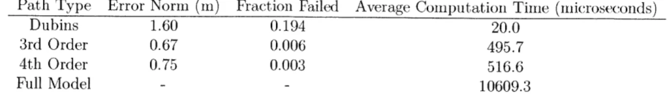
The algorithm for generating the trajectories used in the planning process com-putes a transverse polynomial offset from a nominal Dubins path. The polynomial offset allows us to explicitly specify transverse derivatives in terms of linear equality constraints on the coefficients of the polynomial, and minimize transverse derivatives

by using a Quadratic Program (QP) on the polynomial coefficients. This results in

a computationally cheap method for generating paths with continuous heading, roll angle, and roll rate for the fixed-wing vehicle, which is fast enough to run in the inner loop of the RRBT.

Thesis Supervisor: Nicholas Roy

Acknowledgments

I would like to thank my advisor Nicholas Roy for giving ine the freedom to shape this project while providing his guidance and sharp insight along the way. Thanks to the other members of the Robust Robotics Group and in particular thanks to Abraham Bachrach for being a constant sounding board for algorithmic ideas and software development, and for his direct contributions to the state estimation work in this thesis.

Thanks are due to the Franklin W. Olin Foundation and the entire Olin community for supporting my undergraduate education and setting me down the path that led this work.

My parents, Douglas Bry and Jill Parker, and sister, Leah Bry, are responsible for a foundation of support and a drive towards intellectual inquiry. Any strength in this work is reflective of that foundation and that drive.

Finally, I would to thank my friends, roommates, and the members of the MIT Cycling Team for giving me so much to live for outside of the lab.

Contents

1 Introduction

1.1 Contributions.. . . . ...

1.1.1 Belief Space Planning for Dynamic Systems

1.1.2 State Estimation... . . . . . ..

1.1.3 Trajectory Generation . . . .

1.2 Thesis Overview . . . .

2 Related Work

2.1 Flight Through Obstacles. . . . ..

2.2 Trajectory Generation . . . .

2.3 State Estimation . . . ...

2.4 Motion Planning Under Uncertainty . . . .

3 Trajectory Generation and Control

3.1 Coordinate Frames and Nomenclature . . . .

3.2 Coordinated Flight Model . . . .

3.3 Trajectory Generation.. . . . ..

3.3.1 Quadratic Optimization on the Derivatives of Polynomials

3.3.2 Piecewise Polynomial Joint Optimization . . . .

3.3.3 Polar Coordinates Corrections . . . . 3.3.4 Line Segment Corrections . . . .

3.3.5 Dubins-Polynomial Paths... . . . .. 3.3.6 Path Limitations.... . . . . 9 . . . .. 13 . . . . 14 . . . . 14 . . . . 15 . . . .17 19 . . . . 19 . . . . 2 1 . . . . 23 . . . . 2 5

3.4 C ontrol . . . . 3.4.1 Trajectory Stabilization . . . ....

3.4.2 Differentially Flat Control Input Conversion .

3.5 Simulation Results... . . . . . ...

4 State Estimation

4.1 State Estimation Problem Statement . . . . 4.2 IMU Process Model . . . . 4.2.1 Exponential Coordinates Attitude Uncertainty 4.3 Process Equations . . . . 4.4 Identifying the Process Noise Parameters . . . . 4.4.1 Partioned GPF Measurement Update . . . . . 4.4.2 Laser Localization . . . .

4.5 Experimental Results... . . . . . . . .

5 Rapidly-exploring Random Belief Trees 5.1 Problem Formulation . . . . . . .. 5.2 Uncertainty Prediction . . . . ... 5.3 Rapidly-exploring Random Belief Tree

5.3.1 Comparing Partial Paths . .

5.3.2 Algorithm Description...

5.4 Convergence Analysis . . . ...

5.5 Experimental Results . . . . . . ..

5.5.1 Fixed-wing Vehicle Simulation

6 Future Work and Conclusions

. . . . . . 47 . . . . 48 . . . . 49 . . . . 50 57 . . . . 57 . . . . 58 . . . . 59 . . . . 61 . . . . 63 . . . . 65 . . . . 69 . . . . 70 75 75 77 81 83 84 85 90 93 103

Chapter 1

Introduction

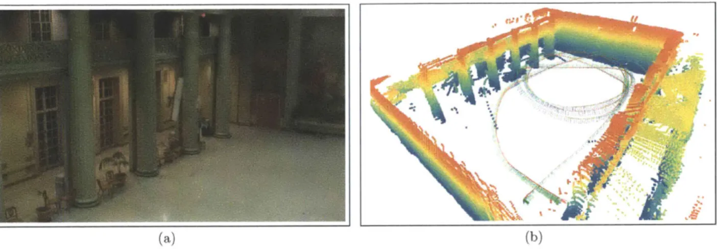
Advances in system identification, control, and planning algorithms increasingly make it possible for autonomous flying vehicles to utilize the full scope of their natural dy-namics. Quad-rotors capable of agile flight through tight obstacles, helicopters that perform extended aerobatic sequences, and fixed-wing vehicles that mimic the perch-ing behavior of birds, have all been reported in the literature [14, 16, 42]. Sinulta-neously, advances in LIDAR and computer vision algorithms have made autonomous flight through obstacle-rich environments possible without the use of an external sen-sor system [4, 3]. Currently, there is growing interest in extending the highly dynamic maneuvers that have been demonstrated when accurate state information is always available to autonomous vehicles that operate in unstructured environments using only on-board sensors.

The central problem that motivates the work in this thesis is the autonomous flight of a small, unmanned, fixed-wing vehicle through an obstacle rich environment using only on-board sensors. This technology would represent a substantial step forward in the state of the art for autonomous systems and be a useful enhancement for the capabilities of existing micro air vehicles (MAVs) which are increasingly deployed in military, search and rescue, and security roles around the world. As we will see, the problem presents unique challenges from a control, state estimation, and planning perspective.

Figure 1-1: Fixed wing experimental platform flying indoors localizing using an on board laser range scanner and inertial measurement unit.

quad-rotor flight through obstacles using on-board sensors is the non-trivial vehicle dynamics. Because helicopters are capable of hovering in place, many of the same algorithms that have advanced the capabilities of ground robots in the last twenty years can be adapted for use in the hover regime [4]. Such is not the case for fixed-wing vehicles. While they share the payload and computation constraints with quad-rotors, a fixed-wing vehicle must maintain a forward velocity to lift the payload, and that velocity scales with the payload. Thus the more computation and sensing power on board an airplane, the faster it must fly for a fixed wing size. This constraint on the minimum velocity places a substantial design burden on anything that must run in real-time on the vehicle: namely the state estimation and feedback control

algorithms. Further, most of the work with quad-rotors using laser range scanners (LIDARs) makes strong 2.5D assumptions about the environment. These assumptions are reasonable on a quad-rotor since the vehicles does not depart from the hover regime where the sensor is close to level in the x-y plane. For a fixed-wing vehicle, maneuvering requires departing the plane -at least in roll, and the tighter and more aggressive the maneuvering, the larger the magnitude of the departure.' True 3D localization using only a planar LIDAR is thus a primary challenge for our vehicle.

One could argue that state estimation is the most significant, direct challenge faced

by a fixed-wing vehicle flying through obstacles using only on-board sensing. However,

difficult state estimation translates directly into challenges in planning. When using on-board sensors, the ability of the vehicle to estimate its position depends on both the position itself and its velocity as obstacles and environmental features come in and out of view of the planar LIDAR. An aggressive bank angle may make localization in the horizontal dimensions difficult or impossible altogether, but allow the vehicle to get accurate height information as LIDAR beams hit the ground. Motion blur and other speed effects cause similar state-dependent localization problems for camera-based sensing if the vehicle executes maneuvers with high velocity or angular rates. Failure to reason intelligently about the state-dependent uncertainty during planning could lead to an unacceptable probability of crashing. A successful planner must have knowledge of what future state estimates may occur, in terms of both mean and uncertainty - the "belief space" of the vehicle. It must make plans that are appropriately cautious when the vehicle will be uncertain about its position while executing trajectories and maneuvers that allow the vehicle to gather information and improve its state estimate when advantageous in terms of overall path cost. By seeking low-cost or optimal paths, information gathering and caution around obstacles become tightly coupled problems. Much previous work in planning under uncertainty focuses solely on finding maximum information or minimum uncertainty paths [24]. In contrast, we are interested in gathering information and reducing uncertainty only

12.5D means the environment is represented as an extrusion in three dimensions of a

if it allows the vehicle to reach the goal more efficiently: if the vehicle can fly a shorter trajectory by temporarily being very uncertain of its location, but an accurate state estimate will be recovered before flying close to an obstacle, that is desirable behavior. To solve the planning problem we propose an asymptotically optimal sampling-based approach sampling-based on recent advances in sampling sampling-based motion planning [29]. Sampling-based approaches - most commonly variants of the Rapidly-exploring Ran-dom Tree (R.RT) or Probabalistic Road Mal) (PRM)- are widely used in robotics: they are easy to implement, computationally efficient, and are often probabilistically complete in the sense that if a solution exists it will be found with probability 1 given enough samples. The algorithm we propose in this thesis, the Rapidly-exploring Random Belief Tree (RRBT) works by incrementally constructing a graph of feasible trajectories through state space and then "propagates" uncertainty along the edges of the graph by simulating state estimation and control along the paths. While pow-erful, this framework introduces additional constraints on the state estimation and control algorithms.

To efficiently propagate uncertainty, we use a Gaussian representation of the state distribution, such that state estimates are fully characterized by a mean and covari-ance matrix. Unfortunately, laser range measurements in three dimensions are gener-ally far from Gaussian in their noise properties. However, the state estimation algo-rithm we propose extends a technique called the Gaussian Particle Filtering (GPF) to use particles (weighted samples in the state space) to capture the non-Gaussian, non-linear laser measurements as Gaussians. This not only makes for a computation-ally efficient state estimator, but also allows these pseudo-Gaussian measurements to be used efficiently during planning.

Sampling-based approaches work by samnpling states and connecting them with feasible trajectories. The approach we use, an extension of the RRT* algorithm (a recent version of the RRT which asymptotically converges to the optimal solution) requires that these connections to sampled states be made exactly. Exact connections ensure that if a lower cost path is discovered to some point in state space, the lower cost alternative trajectory can be substituted in without disturbing the subsequent

trajectory. However, generating exact connections is itself an algorithmic challenge. For our planning algorithm to be successful we must have a method of generating kinodynamically feasible trajectories between two arbitrary states, and this method must be computationally efficient since it will be used each time a state is sampled. We introduce a technique for generating paths based on a differentially flat model of coordinated-flight vehicle dynamics. Differential flatness implies system inputs and states are fully determined by a set of outputs and output derivatives. For the coordinated flight model, the output is the spatial trajectory. This model allows us to generate trajectories using transverse polynomial offsets from a nominal path which minimize the control effort required to follow that path.

Finally, since stochasticity factors prominently into the vehicle dynamics and sens-ing, we must use a feedback control law to stabilize the planned trajectory. In planning we propagate Gaussian uncertainty. To maintain a Gaussian, the dynamics along the path must be linear which is generally not the case for fixed-wing vehicles. However, the differentially flat vehicle model allows us to achieve approximately linear error dy-namics, meaning the uncertainty prediction used in planning can more closely match what can be expected during path execution, as the RR.BT planning algorithm uses closed-loop predictions of the state uncertainty.

Thus the central problem of fixed-wing flight through obstacles motivates algo-rithmic development in state estimation, planning, trajectory generation, and control. Furthermore, we can see that choices and design constraints in one algorithm can in-troduce choices and design constraints in the others. This thesis inin-troduces algorithms for each of these pieces, which while all independently useful and potentially broadly applicable, are specifically motivated and designed to work as a unified system.

1.1

Contributions

This thesis makes contributions in trajectory generation (chapter 3), state estimation (chapter 4), and planning under uncertainty (chapter 5). We outline the contributions below.

1.1.1

Belief Space Planning for Dynamic Systems

The central and unifying contribution of this thesis is a novel algorithm that extends a class of recently proposed incremental sampling-based algorithms to handle state-dependent stochasticity in both dynamics and measurements [29]. The key idea is in leveraging the fact that the incremental sampling approach allows us to enumer-ate all possible paths through an environment to find paths that optimally trade off information gathering, avoiding obstacles, and quickly reaching the goal. To ensure the plan is suitable for systems with nontrivial dynamics, we evaluate paths with a probabilistic distribution over all possible trajectories that may be realized while fol-lowing a path with a closed-loop controller. The algorithm proceeds by incrementally constructing a graph of feedback stabilized trajectories through state space, while ef-ficiently searching over candidate paths through the graph as new samples are added.

We provide a pruning technique that exploits specific properties of uncertainty

prop-agation for eliminating possible paths and terminating search after each sample is added. In the limit, this process results in a tree in belief space (the space of proba-bility distributions over states) that contains the optimal path in terms of minimum cost with a bounded probability of collision or "chance-constraint".

Both sampling-based algorithms and linear control and estimation schemes have been shown to scale well with dimensionality. Additionally, the algorithm has the powerful property offered by incremental sampling algorithms of quickly exploring the space and then provably converging to the optimal solution. This is particularly desirable for stochastic planning problems since they are computationally demanding and in a real-time setting the computational time available could vary widely.

1.1.2

State Estimation

The wide disparity between what is possible in terms of agile flight with an external positioning system and what has been (demonstrated with onboard sensing suggests that state estimation from on board sensors is indeed a significant challenge in ex-tending the capabilities of MAVs in real world environments. In addition to providing

accurate estimates, the state estimation system must also accurately identify its un-certainty in order to enable planning with applicable partially observable motion planning algorithms.

This thesis presents a state estimation method that is suitable for use in real-time on a fixed wing MAV maneuvering through a cluttered environment. Our system leverages an inertial measurement unit (gyros and accelerometers) and a planar laser range finder in a filtering framework that provides the accuracy, robustness, and computational efficiency required to localize a MAV within a known 3D occupancy

grid map.

Our process model is a based on an exponential-coordinates extended Kalman filter that is driven by inertial measurements. Unlike conventional system identi-fication techniques that estimate model parameters from sensor data labeled with ground truth states, the model parameters of the IMU process model are estimated

using an algorithm that does not require access to ground truth data. In order to

efficiently project the nonlinear laser measurement update of the vehicle position back through the state estimate, we integrate the laser range-finder measurement as a pseudo measurement computed from a Gaussian Particle Filter state update in a lower dimensional measurement space. The use of the lower dimensional space drasti-cally reduces the number of particles required, thereby enabling realtime performance in the face of the computational limitations of the flight computer. We demonstrate the effectiveness of our approach experimentally on a fixed wing vehicle being piloted in a challenging GPS-denied environment.

1.1.3

Trajectory Generation

The RRBT planning algorithm requires that we be able to make exact connections between sampled states. We develop an algorithm based on parameterizing a trans-verse polynomial offset from a nominal path which allows us to explicitly optimize and specify the transverse derivatives of that path at intermediate points along the trajectory and at specified start and end locations. For fixed-wing vehicles, these transverse derivatives map directly to heading (first derivative) roll angle (second

derivative or curvature), roll rate (third derivative or derivative of curvature), and roll acceleration (fourth derivative, second derivative of curvature). Our method al-lows us to generate paths that are smooth up to the derivative of curvature (roll rate) and could be extended to higher derivatives if desired.

By explicitly specifying the transverse derivatives at points along a path, we can

"correct" for discontinuities in the underlying path. The ability to match derivatives between segments allows us to use Dubins curves which are continuous only up to heading, but can be generated very quickly using simple geometric calculations, as the nominal paths.2

We optimize the transverse offset to minimize quadratic cost on

the offset and its derivatives which translates into approximate minimization of the control effort - namely roll rate and roll acceleration -necessary to follow the paths, Furthermore, since the transverse offset is represented as a polynomial, the quadratic minimization takes the form of a Quadratic Program (QP) with approximately linear constraints.

We present a solution method based on an initial joint optimization of polynomials for all the segments (lines and arcs) composing a Dubins path with linear constraints between the segments and at the start and end of the path. We then use correction expressions that capture the nonlinearaties in the transverse derivatives induced by the offset, to setup a second optimization for each segment individually to ensure the derivative smoothness of the final path. Both optimization steps take the form of a QP with linear constraints which can be solved in a single step using variable elimination. Thus kinodynamically feasible paths for the fixed wing vehicle representing exact connections in state space are achieved using single-step matrix inversions on matrices with dimension of the order to the polynomial. This computational efficiency makes the trajectory generation suitable for use in the RRBT algorithm.

2While we demonstrate the technique with Dubins curves, transverse polynomial paths could be used for any nominal path including concatenated line segments.

1.2

Thesis Overview

In chapter 2 we survey the literature and give an overview of the prior work that has been done in each of the areas we address algorithmically. Chapter 3 presents the trajectory generation and accompanying control algorithm used for planning. In chapter 4 we describe the state estimation algorithm and present results obtained from hand-flown flight experiments in a challenging indoor environment. Chapter 5 develops the RRBT algorithm, including theoretical proofs for the completeness and asymptotically optimal behavior of the algorithm under reasonable technical assumnp-tions. We demonstrate the algorithm on example problems with single integrator and Dubins dynamics with polygonal obstacles, and we also provide simulation results for plans generated with transverse-polynomial paths and GPF measurements computed in a real three dimensional map of an urban environment. Finally, in 6 we conclude and discuss future work.

Chapter 2

Related Work

In this chapter we survey the literature relevant to the problems addressed in this thesis. The literature survey is organized in much the same way as the thesis itself. We begin by looking at work with similar high level goals: autonomous flight through obstacles. We then analyze related work in each of the algorithmic areas this thesis addresses: trajectory generation, state estimation, and finally motion planning, and specifically motion planning under uncertainty.

2.1

Flight Through Obstacles

The potential benefits of MAVs that can operate safely and reliable in and around obstacles has attracted considerable attention in the research community. The bulk of the work has been done with helicopters, either conventional variable pitch con-figurations or quad-rotor concon-figurations, but more recently some work has been done with fixed-wing vehicles.

Bachrach, He, Prentice, and Roy present one example of a completely autonomous quad-rotor capable of operating in unknown and unstructured environments without the use of GPS [4]. Many of the design decisions in the algorithms presented in this thesis are motivated by this system. The core enabling technology is a high frequency scan matcher that uses successive laser scans from the Hokuyo LIDAR to estimate planar velocity which can be integrated over impressively long time scales

to position. In conjunction with the on-board IMU, the scan matcher forms the backbone of the quad's state estimator, which can then be integrated with higher level full simultaneous localization and mapping (SLAM) solutions [54]. Other quad-rotor systems for flying in GPS-denied environments use very similar system architecture

[52, 18].

While this framework is powerful and has resulted in impressive experimental demonstrations, it is based on flying close to the hover regime where motion plan-ning can be done kinematically (motion plans are essentially constructed as simple line segments) and both estimation and planning are strongly dependent on 2.5D world assumptions. In contrast, our work is aimed at eliminating these assumptions with fully 3D state estimation and trajectory generation and planning that explicitly account for and utilize non-trivial fixed-wing dynamics.

Scherer et al. developed a helicopter system capable of flying at high speeds

(10 m/s) around obtacles based on high accuracy differential GPS combined with

a suite of on-board sensors and collision avoidance algorithms [50]. In contrast, we are interested in enabling this kind of behavior without the use of an external system such as GPS, and with a sensor payload more constrained by the physics of fixed-wing flight.

Much of the experimental work done with fixed-wing vehicles flying in close prox-imity to obstacles using oi-board sensing is based on optical flow from visual sensors

[9, 59]. Much of this work is inspired by the systems insects use to navigate [15].

The essentially idea is a direct mapping from sensory input to control actions. Opti-cal flow is Opti-calculated by estimating pixel motion between camera frames, creating a vector field in image space. Areas of the image where the flow is large in magnitude represent potential close proximity to obstacles, and thus obstacle avoidance can be accomplished by steering away from areas of high optical flow. Such systems have been shown to be stable flying through corridor type environments.

While impressive in many respects, this kind of system is inherently limited. Be-cause sensing is mapped directly to control output, no internal state estimate of the vehicle is maintained. This is highly comnputationally efficient for MAVs as small as

10 grams [59], however, the absence of an internal state estimate makes global, higher

level reasoning difficult. For example it would be difficult to give such a system a command such as "go from point A to point B as quickly as possible while avoiding too high a probability of collision" and have certainty that it could accomplish this task. Furthermore, optical flow has a singularity directly in front of the vehicle -no matter how fast you fly directly at an obstacle, its position in the image frame does not change, which presents an obvious problem for many situations when flying around obstacles since the system is essentially blind to what is directly in front of it. When highly accurate, off-board sensing systems are used for positioning, some extremely impressive, agile flight has been demonstrated. In particular Mellinger et al. designed a system capable of aggressively flying quad-rotors through narrow slits [43]. The system is based on a detailed vehicle dynamics model and the controller and trajectories are hand-tuned and iteratively refined through experiments. All of the work is done in a VICON motion capture system which provides real-time, millimeter-level-accuracy position and orientation of the vehicle at rates over 100Hz. In the fixed-wing regime, Cory et al. designed a system capable of mimicking the perching behavior of birds with small foam gliders [16]. Multiple control methodologies were shown to be successful in achieving perching behavior, but once again all of the work relied on a VICON motion capture system. Both of these systems serve as inspiration for our work in terms of what MAVs are dynamically capable of, but the reliance on on-board sensing necessarily differentiates the algorithms in this thesis.

2.2

Trajectory Generation

The general problem of "steering" a dynamics system from one state to another is the subject of a great deal of work in optimal control. For very simple linear systems the solution can be obtained as the solution of a linear system of equations [8]. In contrast, in the most general case for nonlinear systems, solutions can be computed via shooting methods or direcy collocation [57]. While powerful, these methods rely on decomposing a trajectory into a discrete "control tape" of actions which are played

back to execute the trajectory, and the entire control tape is then optimized to satisfy the boundary conditions and minimize an objective function. In general, this results in a non-convex, nonlinear optimization problem with dimension equal to the number of control steps which can be enormous depending on the resolution required by the system. Tedrake uses similar techniques to drive a sampling-based motion planning system, but that work is specifically designed to maintain a sparse tree with feedback control laws, such that the number of trajectories that need to be computed is small (since they are coinputationally expensive). In controls, the asymptotically optimal properties of our planner rely on a dense population of state space with samples and trajectories. Thus, a more efficient means of computing trajectories is required.

The simplest technique in use for fixed-wing vehicle motion planning is Dubins curves [38]. While powerful, and extremely fast to compute, Dubins curves are only continuous in heading and have discontinuities in curvature, which corresponds to dis-continuities in roll angle. For vehicles flying high above obstacles with a conservative radius used in Dubins arcs, this is not a problem as the controller can stabilize the vehicle back onto the path [33]. However, if we wish to use the full dynamic envelope, a different technique is required.

Spline curves - _{piecewise, independent polynomials in each dimension - are a} potentially appealing choice. Mellinger et al. use "minimum-snap" spline curves for their quad-rotor vehicles flying in and around obstacles [41]. However, this technique is not directly applicable to planning for a fixed-wing vehicle.

Most importantly, splines do not respect curvature constraints and do not have constant velocity norm along a path. Pythagorean hodographs overcome these is-sues by maintaining a "perfect square" property of polynomials along a path such that c(t) = N/a(t)2 +

b(t)

curves may be arbitrarily smooth, the transverse derivatives, which are what we care about for control effort to follow the paths, are not explicitly specified in the path formulation.

Another alternative is to use clothoid-are segments which stitch together Dubins curve segments (arcs and lines) with segments of continuously varying curvature [55].

While better than Dubins curves, this would result in paths where the vehicle either has zero roll rate or rolls at some pre-specified maximum roll rate corresponding to the derivative of curvature.

Our approach leverages the advantages of splines presented by Mellinger et al., but extends this functionality by defining a transverse offset from a nominal path that captures the basic shape of the desired trajectory, allowing for explicit control

(both specification and optimization of) the transverse derivatives.

2.3

State Estimation

State estimation using Kalman filtering techniques has been extensively studied for vehicles flying outdoors where GPS is available. A relevant example of such a state estimation scheme developed by Kingston et al. [32] involves two Kalman filters where roll and pitch is determined by a filter driven by gyro measurements as inputs and where the accelerometer measurements are treated as a measurement of the gravity vector, assuming unaccelerated flight. A separate filter estimates position and yaw using GPS measurements.

This approach is representative of many IMU based estimators that assume zero acceleration and thus use the accelerometer reading as a direct measurement of at-titude (many commercially available IMUs implement similar techniques on-board using a complementary filter). While this approach has practical appeal and has been successfully used on a number of MAVs, the zero acceleration assumption does not hold for general flight maneuvering and thus the accuracy of the state estimate degrades quickly during aggressive flight.

Van der Merwe et al. use a sigmna-point unscented Kalman filter (UKF) for state estimation on an autonomous helicopter [56]. The filter utilizes another typical ap-proach whereby the accelerometer and gyro measurements are directly integrated to obtain position and orientation and are thus treated as noise perturbed inputs to the filter. Our filter utilizes this scheme in our process model, however we use an EKF with exponential coordinates based attitude representation instead of the quaternions

used by Van der Merwe et al.

Techniques to identify the noise parameters relevant for the Kalman filter emerged not long after the original filter, however the most powerful analytical techniques assume steady state behavior of a linear time invariant system and are thus unsuitable for the time varying system that results from linearizing a nonlinear system [40]. More recent work optimizes the likelihood of a ground-truth projection of the state over the noise parameters but thus requires the system be fitted with a sensor capable of providing ground-truth for training. [2]. Our algorithm does not require the use of additional sensors, or external ground truth.

Laser range finders combined with particle filter based localization is widely used in ground robotic systems [53]. While planar LIDARs are commonly used to estimate motion in the 2D plane, they have also proved useful for localization in 3D environ-ments. Prior work in our group [5], as well as others [51, 22] leveraged a 2D laser rangefinder to perform SLAM from a quadrotor in GPS-denied environments. The systems employ 2D scan-matching algorithms to estimate the position and heading, and redirect a few of the beams in a laser scan to estimate the height. While the systems have demonstrated very good performance in a number of realistic environ-ments, they must make relatively strong assumptions about the motion of the vehicle, and the shape of the environment. Namely, they require walls that are least locally vertical, and a mostly flat floor for height estimation. As a result, the algorithms do not extend to the aggressive flight regime targeted in this paper. Scherer et al. use laser rangefinders to build occupancy maps, and avoid obstacles while flying fast through obstacles [49], however they rely on accurate GPS measurements for state estimation, and do not focus oi state estimation.

In addition to the laser based systems for GPS-denied flight, there has been a significant amount of research on vision based control of air vehicles. This includes both fixed wing vehicles [31], as well as larger scale helicopters [12, 30, 27]. While vision based approaches warrant further study, the authors do not address the chal-lenge of agile flight. This is likely to be particularly challenging for vision sensors due to the induced motion blur, combined with the computational complexity of vision

algorithms.

Recently, Hesch et al. [26] developed a system that is similar in spirit to ours to localize a laser scanner and INS for localizing people walking around in indoor environments. They make a number of simplifying assumptions such as zero velocity updates, that are not possible for a fixed-wing vehicle. Furthermore, they model the environment as a set of planar structures, which limits the types of environments in which their approach is applicable. Our system uses a general occupancy grid representation which provides much greater flexibility of environments.

2.4

Motion Planning Under Uncertainty

The general motion planning problem of trying to find a collision-free path from some starting state to some goal region has been extensively studied. In particular, sampling-based techniques have received much attention over the last 15 years. The

Rapidly-exploring Random Tree (RRT) operates by growing a tree in state space, iteratively sampling new states and then "steering" the existing node in the tree that is closest to each new sample towards that sample. The RRT has many useful prop-erties including probabilistic completeness and exponential decay of the probability of failure with the number of samples [37].

The Rapidly-exploring Random Graph (RRG) proposed by Karaman and Frazzoli is an extension of the RRT algorithm [29]. In addition to the "nearest" connection, new samples are also connected to every node within some ball. The result is a connected graph that not only rapidly explores the state space, but also is locally refined with each added sample. This continuing refinement ensures that in the limit of infinite samples, the RRG contains all possible paths through the environment that can be generated by the steering function used to connect samples. The RRT* algorithm exploits this property to converge to the optimal path by only keeping the edges in the graph that result in lower cost at the vertices with in the ball. While these algorithms have many powerful properties, they assume fully deterministic dynamics and are thus unsuitable for stochastic problems in their proposed form.

Partial observability issues pose severe challenges from a planning and control perspective. Computing globally optimal policies for partially observable systems is possible only for very narrow classes of systems. In the case of discrete states, actions, and observations, exact Partially Observable Markov Decision Process (POMDP) algorithms exist, but are computationally intractable for realistic problems [28]. Many approximate techniques have been proposed to adapt the discrete POMDP framework to motion planning, but they still scale poorly with the number of states, and the prospect of discretizing high-dimensional continuous dynamics is not promising [48].

For systems with linear dynamics, quadratic cost, and Gaussian noise properties

(LQG), the optimal policy is obtained in terms of a Kalman filter to maintain a

Gaussian state estimate, and a linear control law that operates on the mean of the state estimate [8]. While global LQG assumptions are not justified for the problems we are interested in, many UAVs operate with locally linear control laws about nominal trajectories, and the Kalman filter with various linearization schemes has proven successful for autonomous systems that localize using on-board sensors [4].

The Belief Road Map (BRM) [47] explicitly addresses observability issues by simu-lating measurements along candidate paths and then choosing the path with minimal uncertainty at the goal. However, the BRM assumes the mean of the system is fully controllable at each time step, meaning that while the path is being executed, the controller is always capable of driving the state estimate back to the desired path. This assumption is valid only for a vehicle flying slowly and conservatively such that dynamic constraints can be ignored. Platt et al. [46] assume maximum likelihood observations to facilitate trajectory optimization techniques and then replan when the actual path deviates past a threshold.

The notion of chance-constrained motion planning is not new. A method of allo-cating risk for fully observable systems is discussed by Ono et al. [44]. Evaluating a performance metric over a predicted closed-loop distribution for partially observable systems was described by van den Berg et al. [6] and also derived independently by the authors [10], while He et al. [25] use a similar technique with open-loop action sequences. The algorithm proposed by van den Berg et al., termed LQG-MP, picks

the best trajectory in terms of minimum cost with a bounded probability of colli-sion from an RRT. However, Karaman and Frazzoli show that the RRT in essence enumerates a finite number of paths, even in the limit of infinite samples [29]. Thus there is no guarantee that a "good" path will be found either in terms of cost or un-certainty properties. In fact, we provide an example problem where an RRT fails to find a solution that satisfies chance-constraints, even though one exists. In contrast,

by searching over an underlying graph our approach is both complete and optimal as

the graph is refined in the limit.

Search repair after the underlying graph changes is discussed by Koenig et al. [34], however that algorithm is used for deterministic queries, and our search techniques make direct use of covariance propagation properties. Censi et al. [13] and Gonzalez and Stentz [21] use search with a similar pruning technique, however both algorithms operate on static graphs and do not consider dynamic constraints. We extend the pruning strategy for dynamic systems (i.e., a non deterministic mean) and also use the pruning strategy in the context of an incremental algorithm to terminate search.

Chapter 3

Trajectory Generation and Control

In this chapter we develop the transverse-polynomial trajectory generation technique.

algorithm and returns a dynamically feasible path between the configurations while

optimizing for the control effort (prinmarily in roll) necessary to follow that path. The

algorithm "steers" the vehicle between two points in state space by optimizing the

3.1

Coordinate Frames and Nomenclature

In this thesis we will primarily concern ourselves with only two coordinate frames. A

static global frame, denoted by subscript, g, is a static east-north-pp (xyz) coordinate

frame anchored at some origin. A body frame has its origin at the center of mass

of the vehicle and is oriented x forward, y left, and

z

up (FLU). The transformation

between the two frames is given by a vector, A, between the origins expressed in the

global frame and an orientation given by R. The xyz components of any 3-vector

quantity will be subscripted numerically as 1 for x, 2 for y, and 3 for

z.

This is

'The use of the ENU-FLU coordinate frame runs counter to conventional aeronautical analysis, however, it is in-line with more recent work done with quad-rotors operating indoors (which likely inherit z-up coordinate frames from ground robots) and the choice was made to make easier use of existing software libraries for mapping and visualization.

Figure 3-1: The velocity, body, and global frames depicted with XYZ axes in red,

green, and blue respectively. The global frame ENU global frame is fixed to the

ground with x pointing east). The body frame is fixed to the vehicle with x pointing

out the nose. The velocity frame, assuming coordinated flight, shares the y-axis with

the body frame and has the x-axis aligned with velocity. With positive angle of attack

as shown in this picture, the x-axis points down relative to the body.

We will primarily represent acceleration, angular velocity, and linear velocity in

body coordinates. However, in this chapter exceptions apply. For our coordinated

flight model it is sometimes convenient to discuss velocity and acceleration in the

global frame. In these cases we will refer to derivatives of position for clarity (i.e.,

z/).

Additionally, in this chapter we will use a velocity frame which shares the origin

with the body frame, but has its x axis aligned with the body velocity, while the y

and

z

axes still point left and up respectively as depicted in figure 3-1.

b3

v1

G

v2, b2

3.2

Coordinated Flight Model

The planning and control algorithms for the fixed wing vehicle are based on a coordi-nated flight model [23). Coordicoordi-nated flight is defined as a flight condition where the body velocity of the vehicle is contained within the longitudinal plane, Vb2 = ov2 = 0

and hence iby = 0. The equations of motion for the coordinated flight model are expressed in the velocity frame which differs from the body frame by the angle of attack of the vehicle (assuming the vehicle is in a state of coordinated flight). The orientation of the velocity frame is given by the rotation matrix Rv in

Forward-Left-Up (FLU) to East-North-Forward-Left-Up (ENU) coordinates. The unit vector of the first column

aligns with the velocity, v,2 = vos = 0, the unit vector of the second column points out the left wing, and the unit vector of the third column points up. We also have A Rovv and A g+Rva,,. To maintain coordinated flight, the y and z components of velocity are constrained as:

Lv2 = -(av 3 + go3 )/V (3.1)

-v3

= ge2/1, (3.2)

where gv = Reg and V =|11v, = v,1 =||AI.

A system is differentially flat if the inputs and states can be written as functions

of the outputs and their derivatives. The coordinated flight model is flat with inputs (wv0 i,l

,

avs),

A,

expressed:

1Vi

-W

a

1 0 0

Wvi

I

W3av1/av3

+ 0 -1/av3

0 RS.

(3.3)

ava

Jv2avi

0

0

1

Equation 3.3 is remarkably powerful. It tells us the necessary inputs for the simplified coordinated flight model to achieve an arbitrary third derivative on the trajectory of the airplane. To get intuition about how the differentially flat model,

consider straight and level steady state flight with the world and velocity frames aligned for which we have,

aWi -i

Wi

-J2/g

]

(3.4)

yielding that the roll rate is proportional to the lateral (y direction) "jerk" of the path, the derivative of tangential acceleration is the forward "jerk" of the path, and the derivative of normal acceleration is the upward "jerk" of the path. Thus for a trajectory to have a continuous roll rate it must be smooth up to the 3rd derivative.

3.3

Trajectory Generation

Excepting takeoff and landing maneuvers, we restrict the motion of the vehicle to be in the plane at a constant altitude and fixed speed. For planning purposes we wish to be able to generate trajectories from an initial position, (Ai, A2), yaw angle, ',

roll angle, 0, and roll rate

#

Trajectory generation in the plane must primarily be concerned with roll dynamics as the pitch is effectively constrained to stay in the plane, rudder is constrained to maintain coordinated flight, and throttle is constrained to maintain constant speed. For the case of constant speed planar motion,

V2K

#

is a special case of equation 3.3, where , is the curvature of the path (inverse radius, positive turning to the left or counter clockwise (CCW)).

The most commonly used approach for planar path planning for fixed wing vehicles is to use Dubins curves [38]. Dubins curves represent the optimal (shortest distance) path between two position and orientation, (Ai, A2,@), configurations respecting a

up three path segments consisting of either arcs (of the minimum turning radius) or straight lines, belonging to six possible "words", LSL, RSR, RSL, LSR, RLR, LRL, where L is a left turning arc, R. is a right turning are, and S is a straight line. The parameters of the segments (center, entry and exit angles for an arc, and start and end point for a line) can be directly determined from the geometry of the start and end configurations for each feasible word for a given configuration and then the shortest word selected. It is also possible to analytically determine which word will be shortest based on an algebraic partitioning of SE2, but for implementation simplicity we use the former method.

Since Dubins curves are composed of tangent lines and arcs, the curves are smooth in the sense that a vehicle following the path will have continuous yaw angle, but the curvature is discontinuous. We can see from equation 3.5 that discontinuity in cur-vature will translate to discontinuity in roll angle. This is clearly kinodynamically infeasible for a fixed wing vehicle. However, if the radius is chosen conservatively relative to the roll dynamics of the vehicle and the vehicle is not in close proximity to obstacles, Dubins curves provide a good approximation to kinodynamically feasi-ble paths and a stabilizing controller can achieve reasonafeasi-ble tracking performance. Unfortunately, these conditions do not apply for the system we are interested in as we seek to make use of the full dynamic range of the vehicle while flying close to obstacles.

Differentiating equation 3.5, the roll rate is given by:

V3_k

g = (v .__ (3.6)

The roll angle is a 2nd order system on aileron input [45]. For a truly kinodynamically feasible path we must have continuity up to the derivative of curvature. Clothoid are paths are an extension of Dubins paths with clothoid are segments stitching the lines and arc segments together to maintain continuous curvature (roll angle)

[38).

maneuvering would take place. As with the turning radius, this could be chosen conservatively at the expense of utilizing the full dynamic envelope. In addition, this kind of bang-bang control runs counter to how systems naturally behave. Minimum-snap trajectories, that is trajectories optimized to minimize quadratic cost on the 4th derivative and higher, have been shown to be successful for aggressive flight with quadrotors in highly constrained environments [41].

The roll angle and derivatives can be loosely approximated as,

v26 # ~(3.7) g - ~(3.8) 9 .. _{V4 k} (3.9) 9

While this is clearly an approximation as in general roll angles can be greater than 450, it gives the necessary intuition that minimizing the first and second derivatives of curvature for a path will translate to minimizing the roll rate and roll acceleration.

A quadrotor is capable of "rolling" about any axis in the body's horizontal plane

and thus minimizing the snap or 4th derivative of independent splines in three di-mensions (with a 4th spline for heading) will minimize the control effort to follow the path. This is exactly the method used by Mellinger et al. [41]. For a fixed wing vehicle, however, the picture is substantially more complicated. The axis along which roll acts rotates with the heading of the vehicle and the vehicle must turn with a finite radius, all while traveling at a constant or close to constant speed. This makes the independent axes spline method inapplicable.

The key idea of our approach is in paramncterizing a lateral offset from a nominal path, and using this offset to optimize (minimize) the lateral dynamics quantities we care about.

3.3.1

Quadratic Optimization on the Derivatives of

Polyno-mials

Let p, denote the coefficients of a polynomial P of degree N such that

(3.10) (3.11)

n=p0

We are interested in optimizing the coefficients of P to minimize cost functions of the form

j =

coP(t)

_{+ c1P'(t)}

_{+ c2P"(t)2 + ...}

_p(N)

_(t)

dt,

which can be written in quadratic form as,

J

p

Qp

where

E

Q

=

yN

Cost Matrix and Constraints

The square of a polynomial, p2, can be written using a convolution sum

N

(p2 )n = [pipig.

j=0

The rth derivative is given by

N r-1

P(')(t)

=

( H

Using equations 3.14 and 3.15 we can write the rth component of the cost as a quadratic function of the polynomial coefficients:

- m)) (j - in) ) Ptj-(j- m)( pJ' -(2N N (r-1 M)( n=0 j=0 'm=0 2N N r -1l n=0 j=0 mn=0 - m)) PjPn 2 dt

p,_,jtn-j-rdt

Jr=

p(r)

dt

f

nE

We find Qr by taking the Hessian of this expression: &, 4 2N N n=O j=0 2N N n=o j=O 2N N n=O j=O 2N N n=O j=O n-2r+1 P nj(n - 2r + 1) (j m)(n -(r -1 ,m=0 - in) (rn-M)) in)) r-1i ((j - m)(n -j - ma) m=0 (3.22) (3.23) PJPn-j Tn -2r+1

p

(n

-

2r +

1)

+

pi

P

.

2N

(r-1J

H(i-m)(l

-,m)

.2

(]1n0

Similarly, constraints on the value of P and its derivatives can be written as linear functions of the coefficients:

Ap - b = 0. (3.31)

The value of the rth derivative at T is given by:

N P(r)() ₌ n=r

(n

-

m)

pr .

a~pia9pI

For a polynomial segment spanning from 0 to r satisfying derivative constraints on both ends of the interval, A and b are constructed as:

A = ,o b = (3.33) A47 bT Ao, = IM, 0(r i) m :r =n (3..34) 0 : r

fn

(HX'

0:

n<r

Quadratic Program Formulation and Solution

We now have a quadratic program (QP) of the form:

min XTQX

x

s.t. Ax- b= 0

where the decision variables are the polynomial coefficients, x = Since the con-straints are linear we can solve for x directly using the elimination approach [7]. The decision variables are partitioned (and rearranged if necessary) such that the first In (number of constraints) columns of A are linearly independent:

A= B R (3.38)

X

[=

].

(3.39)

This allows us to write XB in terms of XR using invertible B:

XB= B-'(b - RxR). (3.40)

Partitioning

Q

J

[

QRB QRR

+

()

The bTB-TQBBB-lb = J, term is the "penalty" in cost for satisfying the constraints and it does not factor into the location of the optimal solution x*. Substituting

Q'RR = QRR+RTB-T QBBB-R-2RTB-QBR and

fk

J =Je + fxR + XRQRRXR (3.46)

=fR+2Q'RxR (3.47)

DXR

x*

=1

X

B-1(b - Rx*).

(3.49)

low-order polynomial coefficients. The construction of A (equations 3.34 and 3.36) assures the linear independence of these columns. We restrict ourselves to considering problems where derivative constraints are only present sequentially starting with the value of the polynomial (i.e., we don't specify the r+1th derivative if the rth derivative is not specified). We can see from equation 3.48 that QRR must also be invertible (in fact positive-definite) for a unique solution to exist. By equation 3.30 this requires that their exists at least one non zero ci for 0 < i < m meaning that we must have non zero cost on at least one derivative of lower or equal order to m to assure the convexity of the problem. We also note that m will be equal to the number of derivatives (including the Oth) specified at the beginning of the interval plus the number specified at the end.

We now have all the tools necessary to optimize for single polynomials according to quadratic cost on the derivatives and satisfying boundary constraints. Figure 3-2 shows the behavior of the optimization for different parameters.

3.3.2

Piecewise Polynomial Joint Optimization

Since we wish to "correct" for derivative discontinuities in Dubins curves it is neces-sary to jointly _{optimize multiple polynomial segments with specified derivative offsets} between them. A piecewise polynomial path can be constructed as:

Po(t): t < TO

T() 1 P1 (t -7r) _{To~t)T=+<o(3.50)}: ro < t < 'ri + ro (.0

P2

(t

where we define Tk =

E