Cumulative effects in quantum algorithms and quantum process tomography

Cumulative Effects in Quantum Algorithms and

Quantum Process Tomography

by

M

Shelby Kimmel

B.A. Astrophysics

Williams College (2008)

Submitted to the Department of Physics

in partial fulfillment of the requirements for the degree of

Doctor of Philosophy

at the

MASSACHUSETTS INSTITUTE OF TECHNOLOGY

ARCHIVES

ASSACHUETS INSTITUTE OF TECHNOLOLGY

JUL 01 2014

LIBRARIES

June 2014

Massachusetts Institute of Technology 2014. All rights reserved.

~~P)

Author ...

Certified by....

Signature redacted

/

Department of Physics

21, 2014

1

/

May

,Signature

red acted.

'

Edward Farhi

Cecil nd Ida Green Professor of Physics

Thesis Supervisor

Signature redacted

Accepted by...

Krishna Rajagopal

Physics Professor

Associate Department Head for Education

Cumulative Effects in Quantum Algorithms and Quantum

Process Tomography

by

Shelby Kimmel

Submitted to the Department of Physics on May 21, 2014, in partial fulfillment of the

requirements for the degree of Doctor of Philosophy

Abstract

This thesis comprises three results on quantum algorithms and quantum process tomography.

In the first section, I create a tool that uses properties of the quantum general adversary bound to upper bound the query complexity of Boolean functions. Using this tool I prove the existence of 0(1)-query quantum algorithms for a set of functions called FAULT TREES. To obtain these results, I combine previously known proper-ties of the adversary bound in a new way, as well as extend an existing proof of a composition property of the adversary bound.

The second result is a method for characterizing errors in a quantum computer. Many current tomography procedures give inaccurate estimates because they do not have adequate methods for handling noise associated with auxiliary operations. The procedure described here provides two ways of dealing with this noise: estimating the noise independently so its effect can be completely understood, and analyzing the worst case effect of this noise, which gives better bounds on standard estimates.

The final section describes a quantum analogue of a classical local search algo-rithm for Classical k-SAT. I show that for a restricted version of Quantum 2-SAT, this quantum algorithm succeeds in polynomial time. While the quantum algorithm ultimately performs similarly to the classical algorithm, quantum effects, like the observer effect, make the analysis more challenging.

Thesis Supervisor: Edward Farhi

Acknowledgments

I am indebted to many people who helped make this thesis and my research possible. To my advisor, Edward Farhi for his constant support, and for introducing me to so many exciting projects and people. To my thesis committee Peter Shor and Isaac Chuang, for feedback on issues ranging far beyond the contents of this thesis. To my many wonderful collaborators, Avinatan Hassidim, Bohua Zhan, Sam Gutmann, Andrew Childs, Robin Kothari, Marcus da Silva, Easwar Magesan, Isaac Chuang, Kristan Temme, Aram Harrow, Robin Blume-Kohout and Edward Farhi, for helping me to grow as a researcher by teaching me, challenging me, and encouraging me. To Scott Aaronson and Aram Harrow, for always making time to talk, whether about science or life.

I also want to thank all those people who helped me to maintain a vibrant work-life balance. For that I owe a debt to all of my friends, but especially to John Lee and Youbean Oak for drumming with me even when they probably didn't want to, and to my fellow CTP students, especially Ethan Dyer, Mark Mezei, and Jaehoon Lee, for always bringing their lunches back to Building 6 to eat with me. I'm grateful to my family, who has cheered me on in all my endeavors, and sat through more quantum computing talks that any non-scientist ever should. Finally I could not have done this without my supportive and loving husband, Paul Hess, with me every step of the way.

My work was supported by NSF Grant No. DGE-0801525, IGERT: Interdisci-plinary Quantum Information Science and Engineering, by the U.S. Department of

Energy under cooperative research agreement Contract Number DE-FG02-05ER41360, as well as Raytheon BBN Technologies Internal Research and Development.

Attributions and Contributions

Some of this thesis is taken from previously published material. When this is the case, a footnote at the beginning of the chapter will note which sections are taken from published papers. Some of this work has been done in collaboration with others. At the end of each chapter I have included a section in which I describe my contri-butions to that chapter. I have only included work in which I am a sole or significant contributor.

Contents

1 Introduction 13

1.1 The Quantum Computer and the Beach . . . . 13

1.2 Three-For-One Thesis . . . . 16

1.2.1 Composed Algorithms and the Adversary Upper Bound . . . . 16

1.2.2 Robust Process Tomography . . . . 18

1.2.3 Algorithm for Quantum k-SAT . . . . 20

1.3 A Very Brief Introduction to the Notation and Mathematics of Quan-tum Computing . . . . 22

1.3.1 Quantum Algorithms . . . . 23

2 Quantum Adversary Upper Bound 25 2.1 Introduction . . . . 25

2.2 A Nonconstructive Upper Bound on Query Complexity . . . . 27

2.3 Example where the Adversary Upper Bound is Useful . . . . 29

2.4 Non-Optimal Algorithm for Composed FAULT TREES . . . . 33

2.4.1 Set-U p . . . . 33

2.4.2 Span Program Algorithm . . . . 38

2.4.3 Direct Functions . . . . 42

2.5 Optimal Span Program Algorithm for CONSTANT-FAULT TREES . . 43

2.6 Conclusions . . . . 47

2.7 Acknowledgements . . . . 48

3 Robust Randomized Benchmarking 49

3.1 Introduction . . . . 49

3.2 Completely Positive Trace Preserving Maps: Notation and Properties 51 3.3 Randomized Benchmarking of Clifford Group Maps . . . . 53

3.3.1 RB Sequence Design . . . . 56

3.4 Tomographic Reconstruction from RB . . . . 57

3.4.1 Example: Single Qubit Maps . . . . 60

3.4.2 Beyond Unital Maps . . . . 63

3.5 Fidelity Estimation Beyond the Clifford Group . . . . 64

3.5.1 Average Fidelity to T . . . . 65

3.5.2 Average Fidelity to More General Unitaries . . . . 67

3.6 Bounding Error in Average Fidelity Estimates . . . . 69

3.6.1 Bounds on Average Fidelity of Composed Maps . . . . 70

3.6.2 Confidence Bounds on Fidelity Estimates . . . . 71

3.7 Experimental Implementation and Analysis . . . . 74

3.7.1 RBT Experiments . . . . 75

3.7.2 QPT Experiments . . . . 78

3.7.3 DFE Experiments . . . . 80

3.7.4 Bootstrapping . . . . 81

3.7.5 Experimental Results . . . . 83

3.8 Summary and Outlook . . . . 88

3.9 Acknowledgments . . . . 89

3.10 Contributions . . . . 90

4 Quantum Local Search Algorithm for Quantum 2-SAT 91 4.1 Introduction . . . . 91

4.2 Analysis of the Quantum Algorithm for Restricted Clauses . . . . 94

4.2.1 Runtime Bound for the Algorithm . . . . 95

4.2.2 Solving the Quantum 2-SAT Decision Problem . . . . 99

4.3 Conclusions . . . . 103 4.4 Contributions . . . . 104

A Fault Trees and the Adversary Upper Bound 105

A.1 Direct Functions and Monotonic Functions . . . . 105 A.2 Trivial Inputs to Direct Functions . . . . 106 A.3 Composition Proof . . . . 107

B Robust Process Tomography 113

B.1 Unital Maps and the Linear Span Of Unitary Maps . . . . 113 B.2 Reconstruction of the Unital Part with Imperfect Operations . . . . . 115 B.3 Complete-Positivity of the Projection of Single Qubit Operations onto

the Unital Subspace . . . . 116 B.4 Bounds on Fidelity . . . . 120 B.5 Ordering Of Error Maps . . . . 121

C Quantum 2-SAT with Less Restricted Clauses 125

Chapter 1

Introduction

1.1

The Quantum Computer and the Beach

Quantum computers are a tantalizing technology that, if built, will change the way we solve certain difficult problems. Quantum computers replace the bits of a classical computer with quantum 2-dimensional systems (qubits), replace the standard logi-cal operators AND _{and NOT with a set of unitary operations (such as HADAMARD,} PHASE, and C-NOT), and replace read-out with quantum measurement. With these

substitutions, one finds that certain computational problems can be solved in less time with a quantum computer than with a classical computer. The two most well known examples of quantum speed-ups are Shor's factoring algorithm [681 and Grover's search algorithm [34], but the number of quantum algorithms is growing', and several new algorithms are included in this thesis.

Even though a working quantum computer may be many years away, already the ideas of quantum computation have revolutionized the way we think about computing and have broadened the toolbox of computer scientists. Quantum computers have forced a rewrite of the topography of computational complexity theory. Moreover, tools from quantum computing are proving useful in the classical world. For example, given a Boolean function

f,

there are not many classical tools available to determine

'See Stephen Jordan's quantum algorithm zoo for a fairly complete list: http://math.nist.gov/ quantum//zoo.

how many fan-in AND and OR gates are needed to represent

f

as a formula. However, given an upper bound on the quantum query complexity of

f,

one can immediately obtain a lower bound on the number of gates needed to express f as a formula [19]. For a survey of applications of quantum techniques used in classical proofs, see Ref. [27].

Two great challenges for quantum computer scientists are to determine the compu-tational power of quantum computers, and to engineer physical systems whose error rates are low enough that quantum computing is possible. This thesis will address both these topics; we study and analyze several quantum algorithms, giving insight into the computational power of quantum computers, and we describe new methods for accurate quantum tomography, which has implications for the design of improved quantum systems.

Understanding the power and limits of quantum computation is closely related to algorithms. Each quantum algorithm gives us a new lens through which to view the interaction between quantum mechanics and computation. For example, differ-ent algorithms take advantage of various features of quantum mechanics, such as teleportation, entanglement, superposition, or the existence of a quantum adiabatic theorem. As we create algorithms that use these features as resources, we learn which elements are necessary for a quantum speed-up. Additionally, through the creation of algorithms, we gain a sense of which types of problems quantum computers are good at, and for which problems there is no quantum advantage. Tools for bounding algorithms make these intuitions more precise; for example, there is a theorem that there is no quantum algorithm that uses exponentially fewer queries than a classical algorithm to evaluate a total Boolean function [9]. In this thesis, we use several new tools to analyze and bound the performance of quantum algorithms.

Quantum process tomography, the characterization of a quantum operation acting on a quantum system, is a critical part of building quantum devices with lower error rates. Current small-scale quantum systems can not be scaled up to create larger quantum computers because their error rates are above the thresholds needed to apply quantum error-correcting codes. (This situation may soon be changing - recently a

super-conducting qubit system was observed to have error rates at the threshold needed to apply a surface code [7].) In order to reduce errors in these quantum systems, it is helpful to be able to accurately characterize the errors that occur. Accurate characterization of errors using quantum process tomography can help to pinpoint sources of noise and suggest methods for reduction or correction. In this thesis, we will describe a process characterization procedure that is more accurate than many standard tomography procedures.

The three stories in this thesis (two on algorithms, one on tomography) are on the surface unrelated, but all take advantage of cumulative effects to analyze and understand the behavior of quantum systems. To understand these cumulative effects, we'll start with an analogy to the beach.

The beaches of Wellfleet, MA are eroding at a rate of about three feet per year [57] as the dune cliff is dragged out to the ocean. With an order of magnitude estimate of 10 waves a minute, each wave accounts, on average, for about 0.1 micrometers of shoreline erosion. The impact of a single wave on erosion is both small and extremely noisy. However, by taking the cumulative effect of millions of waves into account, we can easily estimate the average action of an individual wave, simply by taking a ruler to the beach once a year. Consider if instead we tried to calculate the average erosional power of a single wave by modeling the effect of a wave on the dunes, then averaged over the distribution of possible wave energies and wind speeds, and kept track of the changing dune shapes and sandbar configurations, which themselves depend on interactions with earlier waves. Compared to the ruler on the sand, this method will be computationally difficult and likely inaccurate.

While this example is essentially glorified averaging, the principles prove to be powerful in the quantum regime. We give two examples, one from quantum algo-rithms, and one from quantum process tomography, where observing cumulative ef-fects allows for more accurate characterization of an individual algorithm or quantum process than would be possible through direct observation of that single algorithm or process. We call this the top-down approach.

algorithm, but in fact approaches the problem from a bottom-up approach; to go back to our beach analogy, our approach is akin to estimating yearly erosion by accurately characterizing the effects of a single wave. We apply this bottom-up approach to analyze a quantum algorithm where each step of the algorithm is well understood, yet determining the cumulative effect of many steps of the algorithm is challenging.

In the next sections of this chapter, we introduce the three stories that will be covered in this thesis, focussing on the importance of cumulative effects in each. The final section in this chapter is a brief introduction to some of the basics of quantum computing and quantum algorithms. If you are unfamiliar with those topics, we suggest reading Section 1.3 first.

1.2

Three-For-One Thesis

All three topics in this thesis are related to quantum computing, but the techniques, tools, and goals vary widely between them. However, all three topics deal with cumulative effects in quantum systems.

1.2.1

Composed Algorithms and the Adversary Upper Bound

In Chapter 2, we study the relationship between quantum algorithms for a function and quantum algorithms for that function composed with itself. A composed function

f

k is the function fk =

f

o (fk-1, ... , fk-1), where

f

1 =

f,

and we call

f

the

non-composed function. To learn something about a non-composed function, a natural place to start is to study the non-composed function.

Let's consider a specific example. Suppose we have a Boolean function f that takes n bits as input f : {O, 1}" -+ {0, 1}. Thus fk is a function of nk input bits. We would like to know the number of input bit values to

f

we need to learn in order to correctly predict the output of fk, assuming that we initially do not know the values of any of the input bits. We call this quantity the exact query complexity of

fk. This seems like a difficult problem, but it becomes simple if we know something about f. Suppose we have an algorithm that allows us to predict the output of

f

with

certainty, after learning the values of m input bits, where m < n. Then an obvious strategy to learn the output of

fk

to is to apply the algorithm for

f

at each level of composition. A simple inductive argument on k shows that we can evaluate fk after learning mk bits. This algorithm is not necessarily optimal, but is at least an upper bound.

As this example shows, a bottom up approach is natural for learning about quan-tum algorithms for composed functions, since an algorithm for

f

can produce an algorithm for fk. In Chapter 2, we will show an example of an opposite top-down effect, where an algorithm for fk can provide information about an algorithm for

f.

In particular, we prove a theorem called the Adversary Upper Bound, which allows us to precisely relate the query complexity of an algorithm for a composed function to the query complexity of an algorithm for the non-composed function.

In Chapter 2, we apply the Adversary Upper Bound to a function f with a quan-tum algorithm whose query complexity depends on two different contributions, the size of the function and the structure (which depends on specific properties of the input to

f).

In this algorithm for f, size is the dominant contribution. However, when we look at a similar algorithm for fk, structure is the dominant contribution to query complexity, and size is less important. We show that because size is not a significant factor in the query complexity of the composed function, size must not have been a necessary component in the original algorithm for

f,

and in fact, the query complex-ity of

f

must not depend on size at all. Studying the composed function algorithm allows us to learn something about the algorithm for the non-composed function.

Just as measuring the cumulative effect of many waves can wash out noise or error that might exist in an observation of a single wave, noting properties of a composed algorithm can clarify which parts of the algorithm for the non-composed function are necessary and which parts are noise. In our example, the dependence on depth turned out to be noise, but it was not obvious that this was the case until we analyzed the algorithm for the composed function

1.2.2

Robust Process Tomography

As we mentioned in Section 1.1, quantum process tomography is an important tool for building better quantum computers. However many standard techniques for charac-terizing quantum processes are subject to systematic errors. These systematic errors mean that even if arbitrarily large amounts of data are taken, the results will not converge to an accurate estimate of the process in question.

To see why this is the case, let's consider one of the most straightforward methods for quantum process tomography [22], QPT. In this protocol, we prepare a state, apply the quantum process to be characterized, and then measure the resulting state using a projective measurement. If sufficiently many initial states are used, and if sufficiently many different measurements are made for each initial state, then in principle we can estimate all of the parameters of the unknown quantum process. However, if there is uncertainty in the initial state preparations or measurements, systematic errors and biases will likely be introduced into the estimate.

Key aspects of a QPT procedure are illustrated in Figure 1-1. For example, a common experiment that is performed in QPT is to prepare the state 10), apply

(where E is the quantum process to be characterized), and then measure in the basis {10), l1)}. This idealized experiment is diagrammed in Figure 1-la. However, in a real system, we can not prepare the

10)

state perfectly. In fact, we generally don't even have an accurate characterization of the true state that is prepared. Likewise a perfect

{

0), 1)1 measurement is not realistic for a physical system, and we generally don't have an accurate characterization of the true measurement that is performed.

While Figure 1-la is the idealized experiment, Figure 1-lb shows the experiment that is actually performed. We represent our faulty state preparation as preparing the state 10) perfectly followed by some (at least partially) unknown error process AO, and we represent our faulty measurement as a perfect measurement in the

{

0), 1)} basis, preceded by some (at least partially) unknown error process AOp. The true1

state preparation and measurement can always be written in this form. Now we see that if we assume we have a perfect state preparation and perfect measurement, the

process that we characterize is not E as desired, but AO/1 o C o AO (where o denotes

composition of quantum processes, and the order of application proceeds right to

left).

a) 0 ₁₀₎₁₁₎

b) j)

A

0

C) +) + |+),

-Figure 1-1: We demonstrate a limitation of standard quantum process tomography (QPT) when there are uncertainties in state preparation and measurement. In Fig. (a), we diagram an ideal QPT experiment characterizing a process C by preparing a state 10), applying the process E, and then measuring in the {I0),

I1)}

basis. In Fig. (b), we diagram the true QPT experiment, in which there are errors on state preparation and measurement. In Fig. (c) we show that when state preparation and measurement change, the errors on state preparation and measurement also change. These state preparation and measurement errors produce inaccuracies in the final estimate of E, as well as estimates of C that are often not valid quantum processes.

While errors on state preparation and measurement result in QPT characterizing a different process from the desired one (we estimate AO/1 oSoAO rather than C), what is worse is what happens when we prepare a different state or measure in a different measurement basis. As before, these states and measurements have errors associated with them, but importantly, these are different errors than the errors associated with the state preparation 10) and the measurement

{10),

1)}. We see this in Figure 1-ic where the state preparation

+)

is associated with the error A+ and the measurement

{

+7),

1-)} is associated with the error A+/-. Now not only are we characterizing Ai o C o Ai rather than C, but Ai and Aj change as state preparation and measurement

change. If we assume that all state preparations and measurements are perfect, then not only will we get an inaccurate estimate of 8, but the estimate will often not be a valid quantum process.

We see that QPT is not robust to uncertainties in state preparation and measure-ment. We would like a protocol that is robust - that produces an accurate estimate of E even when there are uncertainties in state preparation and measurement. In Chap-ter 3 we create a robust protocol using cumulative effects. Instead of acting with E a single time between state preparation and measurement, we apply E multiple times. By doing this in a clever way, we can separate the signal due to E from the noise of state preparation and measurement, resulting in more accurate estimates of 8.

The top-down approach uses cumulative effects to separate out which contribu-tions to a process are important and which are not. In Section 1.2.1 we described how we will use a top-down approach to determine which contributions to an algorithm are important and which are unnecessary. Here, we use a top-down approach to sep-arate out which contributions to an experiment are due to the quantum operation we care about, and which are due to noise from state preparation, measurement, or other extraneous operations.

1.2.3

Algorithm for Quantum k-SAT

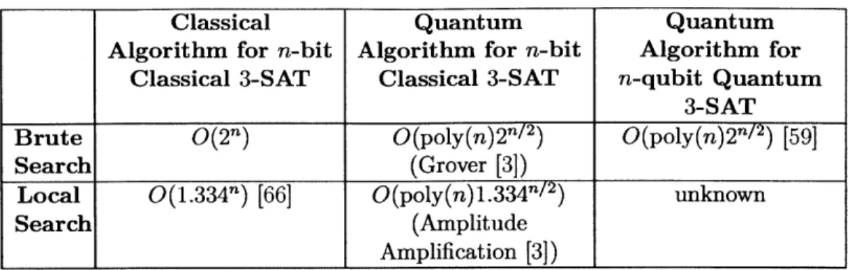
In Chapter 4, we again return our attention to algorithms. In particular we con-sider an algorithm for Quantum k-SAT. Quantum k-SAT is an important problem in quantum complexity because if we can efficiently solve Quantum k-SAT, then we can efficiently solve a host of related and difficult problems [16, 32]. Quantum k-SAT is a quantum version of a classical problem called Classical k-SAT. Both Quantum k-SAT and Classical k-SAT can be solved using a brute force search. A brute force search in-volves searching through all possible solutions to find the correct one. Since there are an exponential number of possible solutions for both Classical k-SAT and Quantum

k-SAT, this takes an exponential amount of time (see the first row of Table 1.1). For Classical k-SAT, using a simple local search algorithm significantly improves the speed of the classical algorithm. A local search algorithm takes the current state

Classical Quantum Quantum

Algorithm for n-bit Algorithm for n-bit Algorithm for

Classical 3-SAT Classical 3-SAT n-qubit Quantum

3-SAT Brute

0(2")

0(poly(n)2n/ 2_{) 0(poly(n)2n/} 2_{) [59]}

Search (Grover [3])

Local

0(1.334n)

[66]

0(poly(n)1.334fn/2)

unknown

Search (Amplitude

Amplification [3])

Table 1.1: Comparing the performance of classical and quantum algorithms for Clas-sical 3-SAT and Quantum 3-SAT. Local search is faster than brute search for ClasClas-sical 3-SAT with a quantum or classical computer, but we don't know how helpful a local search will be for solving Quantum 3-SAT on a quantum computer.

of the system and does a search among states that are similar to the current state. The local search technique also speeds up solving Classical k-SAT using a quantum computer. (See the second column of Table 1.1). However, it is unknown whether a local search can improve the performance of a quantum algorithm for Quantum k-SAT, and hence the "unknown" in the bottom right of Table 1.1. In Chapter 4 we investigate whether such a speed-up is possible.

While performing a quantum local search may be faster than brute search, the analysis of the performance of the algorithm is more complex. This complexity seems counterintuitive, because (as we will see in Chapter 4) at each time step, the quantum local search algorithm performs the same simple operation, which we understand completely. However, the algorithm is difficult to analyze because the progress it makes at a given time step depends on the state of the system at that step, producing a non-linear effect. It makes sense that the progress of the algorithm depends on the state of the system: in a local search we look for options that are close to the current state of the system, and if the current state is in a bad position, it might not be possible to find good options to move to.

In Chapter 4, to analyze the quantum local search algorithm, we use a bottom-up approach. As before, we study a cumulative process, but now we have precise

knowledge of a single step and need to extrapolate to determine the aggregate effects. To do this, we study the action of the algorithm in detail, and apply a tracking device that roughly keeps track of the state of the system over time. Using this strategy, we analyze the performance of the algorithm for a restricted version of Quantum 2-SAT, which is the simplest version of Quantum k-SAT.

1.3

A Very Brief Introduction to the Notation and

Mathematics of Quantum Computing

Quantum computers manipulate quantum states. A pure quantum state of n qubits is an element of the d = 2" dimensional complex vector space with 12

-norm equal to 1, and is denoted by IV). Ideal operations that act on quantum states are unitary matrices of dimension d (unitary operations ensure that the norm is preserved). More generally, a probabilistic quantum state p of n qubits is a 2" dimensional positive semidefinite matrix with trace 1. A pure state 10) corresponds to the rank-1 matrix

I#)(V/l

where

(4'

is the conjugate transpose of I$). General quantum processes acting on such n-qubit states are linear operators that take any valid quantum state p to another valid quantum state p'; in other words, they must be completely positive and trace preserving (CPTP). Measurements are collections of positive operators {Mi} whose sum is the identity, and the probability of outcome i is tr(Mp).

One commonly used set of unitary operators are the Pauli operators. We denote the Pauli operators using the symbols o-, ay, and a-, where

0 1 0 -i 1 0

7-

= , o -= , Z- = . (1. 1)

1 0 )(i 0 )(0 -1)

If we have n qubits, we use orf to mean o-' acting on the ith qubit and the identity acting on all other qubits. That is

where d is the d-dimensional identity operator. (If the dimension is clear from con-text, we will write simply I.) Likewise for oy and of. Generalized Pauli operators on

n qubits are operators of the form {I, a', uy, eZ}®f. We label a generic operator of this form by P , while P0 =12n

We often refer to the eigenstates of the Pauli operators:

* 0) and 1) denote the +1 and -1 eigenstates of a.

* +)

and

I-)

denote the +1 and -1 eigenstates of or.

* I

+-) and | -+) denote the +1 and -1 eigenstates of ry.

1.3.1

Quantum Algorithms

A major goal of quantum computing is to prove that quantum algorithms perform better than classical algorithms at a given task. However, there are several ways in which a quantum algorithm can perform better than a classical algorithm. For example, a quantum algorithm can use less work space than a classical algorithm, like Le Gall's quantum streaming algorithm, which requires exponentially less space than a classical algorithm [45]. Alternatively, a quantum algorithm can use less time than the best known classical algorithm, like Shor's factoring algorithm [68]. Another common way to gauge the performance of quantum algorithms is query complexity, which we explain below. In Chapter 2 we will use query complexity as a metric for the performance of our quantum algorithm, while in Chapter 4 we will use time as the metric.

Query complexity can only be used as a metric for algorithms that have oracles. An oracle is a black box unitary that encodes some information x. For simplicity, in this example, we will assume that x is a string of 2' Boolean bits, x = {x1, . .. , X2-}, with Xi E {0, 1}. x is initially unknown to the algorithm, and the goal of the algorithm is to determine f(x) for some function f. Let { Ji)} be the standard 2" orthonormal basis states on n qubits. Then we are given an oracle

Ox

that acts on those n qubits

as

OX|i) = (--1)Xiz). (1.3)

Thus we can apply Ox to the n qubits in order to learn bits of x.

The action of any query algorithm can be viewed as interleaving applications of Ox with unitaries Ut that are independent of Ox. If the starting state of the algorithm is 10o), then we call IV') the state of the system after t steps, where

)= U . .. U₂

OxU1OaIp0).

(1.4)

Then the bounded error quantum query complexity of f, which we denote

Q(f),

is defined as the minimum number of applications of Ox needed to evaluate

f(x)

with high probability, e.g. with probability 2/3, as long as x is taken from some allowed set

X. In other words, the bounded error quantum query complexity of f is the smallest

integer T such that there is some sequence of unitaries {U1, .. . , UT} such that for any X E _{X, there is a measurement of the state 10') that gives the outcome} f(x) with probability 2/3.

There are several powerful techniques for putting lower bounds on query com-plexity, such as the adversary method [2, 4, 39, 46] and the polynomial method [10]. These lower bounding techniques allow us to accurately characterize the query com-plexity of quantum algorithms, and from there, compare quantum query comcom-plexity to classical query complexity. However, it is important to keep in mind that while query complexity is an important theoretic tool, for practical purposes, measures like time and space complexity are more significant.

Chapter 2

Quantum Adversary Upper Bound

1

2.1

Introduction

The general adversary bound has proven to be a powerful concept in quantum com-puting. Originally formulated as a lower bound on the quantum query complexity of Boolean functions [39, it was proven to be a tight bound both for the query complex-ity of evaluating discrete finite functions and for the query complexcomplex-ity of the more general problem of state conversion [46]. The general adversary bound is the culmi-nation of a series of adversary methods [2, 4] used to put lower bounds on quantum query complexity. While versions of the adversary method have been useful for im-proving lower bounds [5, 40, 63], the general adversary bound itself can be difficult to apply, as the quantity for even simple, few-bit functions must usually be calculated numerically [39, 63].

One of the nicest properties of the general adversary bound is that it behaves well under composition [46]. This fact has been used to lower bound the query complexity

1 Section 2.4 and Appendix A.2 are adapted from Zhan, B. et al. "Super-polynomial quantum speed-ups for boolean evaluation trees with hidden structure," Proceedings of the 3rd Innovations in Theoretical Computer Science Conference, 02012 ACM, Inc. http://doi.acm.org/10.1145/2090236.

2090258. The rest of the sections in this chapter and in Appendix A (except for Appendix A.1,

which is unpublished) are taken from Kirmmel, S. "Quantum Adversary (Upper) Bound,' Automata, Languages, and Programming, 02012 Springer Berlin Heidelberg. The final publication is available at http://dx.doi.org/10.1007/978-3-642-31594-7_47. Also from Kimmel, S. "Quantum Adversary (Upper) Bound," Chicago Journal of Theoretical Computer Science 2013 Shelby Kimmel, http:

of evaluating composed total functions, and to create optimal algorithms for composed total functions [63]. Here, we extend one of the composition results to partial Boolean functions, and use it to upper bound the query complexity of Boolean functions, using a tool called the Adversary Upper Bound (AUB).

Usually, finding an upper bound on query complexity involves creating an algo-rithm. However, using the composition property of the general adversary bound, the AUB produces an upper bound on the query complexity of a Boolean function

f,

given only an algorithm for

f

composed k times. Because the AUB is nonconstruc-tive, it doesn't tell us what the algorithm for f that actually achieves this promised query complexity might look like. The procedure is a bit counter-intuitive: we obtain information about an algorithm for a simpler function by creating an algorithm for a more complex function. This is similar in spirit to the tensor power trick, where an inequality between two terms is proven by considering tensor powers of those terms2

.

We describe a class of oracle problems called CONSTANT-FAULT TREES, for which the AUB proves the existence of an 0(1)-query algorithm. While the AUB does not give an explicit 0(1)-query algorithm, we show that a span program algorithm achieves this bound. The previous best algorithm for CONSTANT-FAULT TREES has query complexity that is polylogarithmic in the size of the problem.

In Section 2.2 we describe and prove the AUB. In Section 2.3 we look look at a simple function called the 1-FAULT NAND TREE, and apply the AUB to prove that this function can be evaluated using 0(1) quantum queries. For the remainder of the chapter, we consider more general CONSTANT-FAULT TREES, and go into the application of the AUB in more detail. As described above, to apply the AUB to a function, we need to have an algorithm for that composed function, so in 2.4, we create a quantum algorithm for composed CONSTANT-FAULT TREES. Once we have the algorithm for composed CONSTANT-FAULT TREES, we use the AUB to show that these functions can also be evaluated using 0(1) quantum queries. Because the AUB is nonconstructive, we need to separately find an 0(1)-query algorithm, so in 2See Terence Tao's blog, What's New "Tricks Wiki article: The tensor power trick," http://terrytao.wordpress.com/2008/08/25/tricks-wiki-article-the- tensor-product-trick/

Section 2.5 we describe an optimal algorithm for CONSTANT-FAULT TREES that uses span programs.

2.2

A Nonconstructive Upper Bound on Query

Complexity

The AUB relies on the fact that the general adversary bound behaves well under composition and is a tight lower bound on quantum query complexity. The standard definition of the general adversary bound is not necessary for our purposes, but can be found in [40], and an alternate definition appears in Appendix A.3.

Our procedure applies to Boolean functions. A function f is Boolean if

f

:S -{0, 1} with S C -{0, 1}n. We say

f

is a total function if S = {0, 1} and

f

is partial otherwise. Given a Boolean function f and a natural number k, we define fk, "f composed k times," recursively as fk =

f

o

(k-',.... ,fk-

1), where

f

1 =

f.

Now we state the Adversary Upper Bound (AUB):

Theorem 2.2.1. Suppose we have a (possibly partial) Boolean function f that is composed k times, fk, and a quantum algorithm for fk that requires Q(jk) queries. Then

Q(f)

= O(J), where

Q(f)

is the bounded-error quantum query complexity of f.

(For background on bounded-error quantum query complexity and quantum algo-rithms, see [2].) There are seemingly similar results in the literature; for example, Reichardt proves in [61] that the query complexity of a function composed k times, when raised to the 1/kth power, is equal to the adversary bound of the function, in the limit that k goes to infinity. This result gives insight into the exact query com-plexity of a function, and its relation to the general adversary bound. In contrast, our result is a tool for upper bounding query complexity, possibly without gaining

any knowledge of the exact query complexity of the function.

One might think that the AUB is useless because an algorithm for f k usually comes from composing an algorithm for

f.

If J is the query complexity of the algorithm for f, one expects the query complexity of the resulting algorithm for fk to be at

least jk, as we described in Section 1.2.1. In this case, the AUB gives no new insight.

Luckily for us, composed quantum algorithms do not always follow this scaling. If there is a quantum algorithm for

f

that uses J queries, where J is not optimal (i.e. is larger than the true bounded error quantum query complexity of

f),

then the number of queries used when the algorithm is composed k times can be much less than jk. If

this is the case, and if the non-optimal algorithm for

f

is the best known, the AUB promises the existence of an algorithm for f that uses fewer queries than the best known algorithm, but, as the AUB is nonconstructive, it gives no information as to the form of the algorithm that achieves that query complexity.

We need two lemmas to prove the AUB, both of which are related to the gen-eral adversary bound of

f,

which we denote ADV+(f). ADV+(f) is a semi-definite program that depends on

f.

We will not define it explicitly here as the definition is notation-heavy and not crucial for understanding the ideas in this chapter. (The def-inition of the dual of ADV+ is given in Appendix A.3 and the standard defdef-inition can be found in [39].) Rather, we will focus on the following two properties of ADV+(f):

Lemma 2.2.2. For any Boolean function f : S - {0, 1} with S C {O, 1}" and natural

number k,

ADV (fk) > (ADV (f))k. (2.1)

Hsyer et al. [39] prove Lemma 2.2.2 for total Boolean functions3, and the result is extended to more general total functions in [46]. Our contribution is to extend the re-sult in [46] to partial Boolean functions. While the AUB holds for total functions, the nontrivial applications we discuss involve partial functions. The proof of Lemma 2.2.2 closely follows the proof in [46] and can be found in Appendix A.3.

Lemma 2.2.3. (Lee, et al. [46]) For any function

f

: S - E, with S E Dn, and E, D finite sets, the bounded-error quantum query complexity of f,

Q(f),

satisfies

Q(f)

=

E(ADV+(f)).

(2.2)

3

While the statement of Theorem 11 in [39] seems to apply to partial functions, it is mis-stated; their proof actually assumes total functions.

We now prove Theorem 2.2.1:

Proof. Given an algorithm for f that requires O(J) queries, by Lemma 2.2.3,

ADV(f k) = Qpk). (2.3)

Combining Eq. 2.3 and Lemma 2.2.2,

(ADV+(f))k _ Qpk). (2.4)

Raising both sides to the 1/kth power,

ADV1(f) =

0(J).

(2.5)

We now have an upper bound Lemma 2.2.3 again, we obtain

on the general adversary bound of

f.

Finally, using

Q(f) = O(J).

(2.6)

2.3

Example where the Adversary Upper Bound

is Useful

In this section we describe a function, called the 1-FAULT NAND TREE [75], for which the AUB gives a better upper bound on query complexity than any previously known quantum algorithm. To apply the AUB, we need an algorithm for the composed

1-FAULT NAND TREE. In the next section, we describe an algorithm that solves not only the composed 1-FAULT NAND TREE but a broader class of functions called

CONSTANT-FAULT TREES. In the current section, we focus on the 1-FAULT NAND

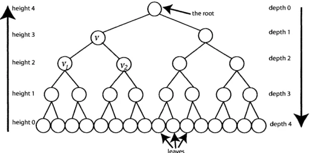
The NAND TREE is a complete, binary tree of depth d, where each node is as-signed a bit value. (For a brief introduction to tree terminology, see Figure 2-1.) The leaves are assigned arbitrary values, and any internal node v is given the value NAND(val(vi), val(v2)), where v, and v2 are v's children, and val(vi) is the value of

the node vi, and NAND is the 2-bit Boolean function whose output is 0 if and only if both inputs have value 1 (Not-AND).

height 4 the root depth 0

height 3 depth 1

height 2 y Vdepth 2

height I depth 3

height 0 depth 4

leavs

Figure 2-1: This is a 2-ary (or "binary") complete rooted tree of depth 4. The circles are called nodes, and one node is labeled as the root. Nodes that are connected to only one other node are called "leaves." Each node is connected to other nodes, some of which are further from the root and some of which are closer to the root. For some node v, we call the nodes that are connected to v but farther from the root the "children" of v. vi and v2 are children of v. This tree is binary because every

node except the leaves has two children. (In an n-ary tree, each node would have n children.) The depth of a node is its distance from the root. The height of a node is depth of that node subtracted from the maximum depth of the tree. This is a complete tree because all of the leaves have the same depth.

To evaluate the NAND TREE, one must find the value of the root given an oracle for the values of the leaves. (The NAND TREE is equivalent to solving NANDd, although the composition we use for the AUB is not the composition of the NAND function, but of the NAND TREE as a whole.) For arbitrary inputs, Farhi et al. showed that there exists an optimal quantum algorithm in the Hamiltonian model to solve the NAND TREE in 0(20.5d) time [30], and this was extended to a standard discrete algorithm

with quantum query complexity O(20--d) [18, 62]. Classically, the best algorithm

requires Q (20.753d) queries [65]. Here, we consider the 1-FAULT NAND TREE, which

is a NAND TREE with a promise that the input satisfies certain conditions.

Definition 2.3.1. (1-FAuLT NAND TREE [75]) Consider a NAND TREE of depth d (as described above), where the values of all nodes are known. Then to each node v, we assign an integer .'(v) such that:

" I(v) = 0 for leaf nodes.

" Otherwise v has children v1 and v2:

- If val(vi) = val(v2), we call v a trivial node, and r(v) = maxiE{1,2} r-(vi),

- If val(vi)

$

val(v2), we call v a fault node. Let vi be the node such that val(vi) = 0. Then n(v) = 1 + r,(vi).

A tree satisfies the 1-fault condition if r.(v) < 1 for any node v in the tree.

The 1-fault condition is a limit on the amount and location of faults within the tree. Whether a tree is a 1-fault tree or not depends on the values of the leaves, as the values of the leaves determine the values of all other nodes in the tree. In a 1-FAULT NAND TREE, if a path moving from a root to a leaf encounters any fault node and then passes through the 0-valued child of the fault node, there can be no further fault nodes on the path. An example of a 1-FAULT NAND TREE is given in Figure 2-2.

The condition of the 1-FAULT NAND TREE may seem strange, but it has a nice interpretation when considering the correspondence between NAND TREES and game trees4. Every NAND TREE corresponds to a two-player game, where the paths from

the root to the leaves correspond to the the possible paths of play, and the values of the leaves determine which of the two players win in that particular end-game. If we evaluate such a NAND TREE, where the values of the leaves determine the possible end-games, then the value of the root of the tree tells which player wins if both players

4

See Scott Aaronson's blog, Shtetl-Optimized, "NAND now for something completely different," http://www.scottaaronson .com/blog/?p=207

play optimally. The NAND TREE is thus a simple example of a problem that can be generalized to understanding more complex two-player games such as chess or go.

With the interpretation of the NAND TREE as a game tree, the more specific case of the 1-FAULT NAND TREE corresponds to a game in which, if both players play optimally, there is at most one point in the sequence of play where a player's choice affects the outcome of the game. Furthermore, if a player makes the wrong choice at the decision point, the game again becomes a single-decision game, where if both players play optimally for the rest of play, there is at most one point where a player's choice affects the outcome of the game. It does not seem farfetched that such a game might exist with practical applications, for which it would be important to know which player will win.

0

V 1

Vi 0 V2 1 0 0

1 1 0 1 1 1 1 1

0 0 0 0 1 1 0 1 1 0 0 1 0 0 0 0

Figure 2-2: An example of a 1-FAULT NAND TREE of depth 4. Fault nodes are highlighted by a double circle. The node v is a fault since one of its children (vi) has value 0, and one (V2) has value 1. Among v, and its children, there are no further

faults, as required by the 1-fault condition. There can be faults among v2 and its

children, and indeed, v2 is a fault. There can be faults among the 1-valued child of

v2 and its children, but there can be no faults below the 0-valued child.

In Section 2.4, we show that there exists an algorithm for the d-depth 1-FAULT NAND TREE that requires 0(d3) queries to an oracle for the leaves. However, when the d-depth 1-FAULT NAND TREE is composed log d times, the same algorithm re-quires 0(d5) queries. Applying the AUB to the 1-FAULT NAND TREE composed log d times, we find:

queries.

Proof. Using our algorithm for composed 1-FAULT NAND TREES, we have that

Q(1-FAULT NAND TREElogd) - 0(d5).

Using Theorem 2.2.1, we have

Q(1-FAULT NAND TREE) = 0(dTg)

5logd

= 0(c Igd)

= O(co)

=0(1)

(

where c is some constant.

2.7)

2.8)

El

Corollary 2.3.1 shows the power of the AUB. Given a non-optimal algorithm that scales polynomially with the depth of the 1-FAULT NAND TREE, the AUB tells us that in fact the 1-FAULT NAND TREE can be solved using 0(1) queries for any depth.

2.4

Non-Optimal Algorithm for Composed Fault

Trees

In this section, we describe a span program-based algorithm for k-FAULT TREES,

of which the 1-FAULT NAND TREE is a specific example. This algorithm is not an optimal algorithm, but will allow us to apply the AUB as in Corollary 2.3.1 to prove the existence of an algorithm with improved performance.

2.4.1

Set-Up

The algorithm for k-FAULT TREES is based on the span program formulation of [631.

span programs and witness size. After laying the groundwork in the current section, in Section 2.4.2 we prove bounds on the performance of the algorithm

Span programs are linear algebraic ways of representing a Boolean function. Every Boolean function can be represented using a span program, and in fact there are an infinite number of span programs that represent a given function. We consider span programs that have a particularly simple form, and we call them direct span programs. The simplified form means that these direct span programs are not general - i.e. not every Boolean function can be represented using direct span programs. Functions that can be represented by these simplified span program are called direct functions.

(For a more general definition of span programs, see Definition 2.1 in [63]).

Definition 2.4.1. (Direct Span Program, adapted from Definition 2.1 in [63]) Let a span program Pf, for a function f : S -+ {0, 1}, S E {0, 1}n, consist of a "target"

vector r = (1,0, ... , 0) and "input" vectors pj for j E {1,. .. ,n}, with T, pf E CN for N E N. We call x the input to f, with x composed n input bits {x1,... , x.}. Each

pt is associated with a single-bit Boolean function Xj that acts on the input bit xj,

where Xj(xj) = xj or xj(xj) = z- depending on the specific function f. The vectors

pj satisfy the condition that f (x) = 1 if and only if there exists a linear combination

of the pj's such that

Z'

ajx,(xj)pj = T, with a3 E C for j E {1,. .. ,n}. Note that if xj(xj) = 0, [ti is effectively not included in the sum. We call A the matrix whose

columns are the pj 's: A = (p,... , p,). Any function that can be represented by such

a span program is called a direct function.

We use input bit to refer to an individual bit input to a function, e.g. xj, while we use input to refer to the full set of input bits that are given to a function, e.g. x.

Compared to general span programs, we have the condition that each input xj corresponds to exactly one input vector - this "direct" correspondence gives the span programs their name. As a result, for each direct function there exists two special inputs, x* and z*: for all of the input bits of x*, Xj(xj) = 1, and for all the input bits of X*, y (xj) = 0. This means x* and z* differ at every bit, f (x*) = 1, f(J*) = 0, and f is monotonic on every shortest path between x* and ;* (that is, all paths of length

n). While all direct functions are monotonic between two inputs x* and z*, not all such monotonic functions are direct functions. We prove this by counterexample in Appendix A.1

One example of direct functions are threshold functions, which determine whether at least h of the n input bits have value 1. Such a threshold function has a span programs where Xj(xj) = xj for

j

E {1,. .. , n}, and where for any set of h input vectors, but no set of h - 1 input vectors, there exists a linear combination that equals r. It is not hard to show that such vectors exist. For threshold functions, ;V* = (0,..., 0) and x* =(,.,)

Given a span program for a direct function, one can create an algorithm with query complexity that depends on the witness size of the span program [63]:

Definition 2.4.2. (Witness Size, based on Definition 3.6 in [63])5 Given a direct function

f,

corresponding span program Pf, input x = (Xi, .. ., Xn), xj E {0, 1}, and a vector s of costs, s E (R)+n, s = (s1,... , sn), let ri be the rows of A (where A is

the matrix whose columns are the input vectors pi of the span program Pf.) ro is the first row of A, r1 the second, and so on. Note ri E Cn. The functions Xi correspond

to the input vectors of Pf, as in Definition 2.4.1. Then the witness size is defined as

follows:

" If f (x) = 1, let w be a vector in Cn with elements wj such that the inner product

row = 1, while riw= 0 for i > 1, and wj = 0 if x,(x) =0. Then

WSIZE(Pf, x) = min s lwl2. (2.9) " If f (x) = 0, let w be a vector that is a linear combination of the vectors ri, with

the coefficient of ro equal to 1, and with wj = 0 if xj(xj) = 1. Then

WSIZE(Pf, x) = min s w3I 2. (2.10)

s

This definition is equivalent to the definition of witness size given in Definition 3.6 in [63]. The reader can verify that we've replaced the dependence of the witness size on A with a more explicit dependence on the rows and columns of A. For the case of f(x) = 0 we use what they call Atw as

Notation: If s = (1,...,1), we write wSIzE1(Pf, x).

We discuss how the witness size is related to query complexity below, but first, we introduce the functions we hope to evaluate.

Consider a tree composed of a Boolean function

f.

The f-TREE is a complete, n-ary tree of depth d, where each node is assigned a bit value. The leaves are assigned arbitrary values, and any internal node v is given the value

f

(val(vi),..., val(v")),

where {vj} are v's children, and val(vi) is the value of the node vi. To evaluate the f-TREE, one must find the value of the root given an oracle for the values of the leaves.

In particular, we consider k-FAULT f-TREES:

Definition 2.4.3 (k-FAULT f-TREES). Consider an n-ary f-TREE of depth d, where throughout the tree nodes have been designated as trivial or fault, and the child nodes of each node have been designated as strong or weak in relation to their parent. All nodes (except leaves) have at least 1 strong child node. For each node v in the tree, let G, be the set of strong child nodes of v. Then to each node v, we assign an integer r,(v) such that:

" r(v) 0 for leaf nodes.

" r(v) = maxbEG., r(b) if v is trivial.

" Otherwise I'(v) = 1 + maxbE Gz(b).

A tree satisfies the k-faults condition if K(v) < k for all nodes v in the tree.

In particular, any tree such that any path from the root to a leaf encounters only k fault nodes is a k-fault tree. Comparing to Definition 2.3.1, it is clear that Defini-tion 2.4.3 is a generalizaDefini-tion of the 1-FAULT NAND TREE. From here forward, for simplicity we call k-FAULT f-TREES simply k-FAULT TREES, but it is assumed that we mean a tree composed of a single function

f,

and where furthermore f is a direct function.

Before our final definitions and lemmas, we need some additional notation. Con-sider an f-TREE of depth d with input x to the leaves of the tree, and conCon-sider a

node v. If v is at height 6, then the value of v is f"(x(v)) where x(v) is the subset of input x assigned to leaves that are descendants of v. We call

f,

the function that determines value of v, so f, = f'. We also need notation for the values of v's children.

If {v1,. . ., v,} are v's children, then x(vi) is the input to the node vi - that is, the

values of the leaves that are descendants of vi. Then

f"(x(v)) = f(f'-1(x(vi),. .. ,f-'1(x(n))), (2.11)

so val(vi) = f6-1 (x(vi)). We denote

2(v) = (f'1 (x(vi)),. . . ( (V)))

= (val(vi), .. . ,val(vn)). (2.12)

We can now relate the query complexity of evaluating a tree composed of composed Boolean functions to the witness size of subtrees of the tree:

Lemma 2.4.1. [Section

4.4

from [63])] Consider an f-TREE of depth d. Consider a node v and its corresponding function fv and input x(v). Let Pf, be a span program corresponding to fv. Then the subformula complexity zf, of the function f, with input x(v), is defined by

z5, (x(v)) < c1 + WSIZEI(P., x(v))(1 + c2E), (2.13)

where c1 and c2 are constants, and E > 0 is a value to be chosen. For a node v that

is a leaf, zj, = 1. Suppose E has the property that E

<

zf,(x(v)) for all nodes v in the tree and for all possible inputs x to f. Then

Q(f) = O(1/E). (2.14)

Finally, we can define trivial, fault, strong, and weak nodes in terms of the witness size and span programs: