HAL Id: hal-02561779
https://hal.archives-ouvertes.fr/hal-02561779
Submitted on 4 May 2020
HAL is a multi-disciplinary open access
archive for the deposit and dissemination of
sci-entific research documents, whether they are
pub-lished or not. The documents may come from
teaching and research institutions in France or
abroad, or from public or private research centers.
L’archive ouverte pluridisciplinaire HAL, est
destinée au dépôt et à la diffusion de documents
scientifiques de niveau recherche, publiés ou non,
émanant des établissements d’enseignement et de
recherche français ou étrangers, des laboratoires
publics ou privés.
Tiltmeter data inversion to characterize a strain tensor
source at depth: application to reservoir monitoring
Severine Furst, Jean Chery, M. Peyret, Bijan Mohammadi
To cite this version:
Severine Furst, Jean Chery, M. Peyret, Bijan Mohammadi. Tiltmeter data inversion to characterize
a strain tensor source at depth: application to reservoir monitoring. Journal of Geodesy, Springer
Verlag, 2020, �10.1007/s00190-020-01377-5�. �hal-02561779�
Tiltmeter data inversion to characterize a strain tensor source at
depth: application to reservoir monitoring
S. Furst
1*, J. Chéry
1, M. Peyret
1, and B. Mohammadi
21GM, Univ Montpellier, CNRS, Univ Antilles, Montpellier, France 2IMAG, Univ Montpellier, CNRS, Montpellier, France.
*now at Univ. Grenoble Alpes, Univ. Savoie Mont-Blanc, CNRS, IRD, IFSTTAR, ISTerre, 38000 Grenoble,
France
Correspondence to: Severine Furst ([email protected])
Abstract.
Surface deformation measured by geodetic data is the sum of single strain sources deforming at depth. A combination of volume changes from several analytical models (e.g. a point source or dislocation along a plane) can be used to model the different sources. However, solving for the best fit of volume variations, dislocations, position and orientation parameters of all sources is a non-linear problem, and its solution is generally non-unique. This problem can be converted into a linear one by assimilating the sum of sources to a simplified model formed by three orthogonal planes of dislocations at fixed position and orientation. This strain source model is equivalent to having all neighbouring deformation sources contained in a small size volume. The determination of the strain tensor components can be performed by inverting geodetic data. Because of their high resolution, tiltmeters are well adapted to survey shallow deformation of volcanoes and geological reservoirs. However, they are known to display unknown long-term drift. We propose an approach to jointly estimate the temporal evolution of the strain source and time-dependent instrumental parameters. We verify the approach using synthetic data, giving confidence intervals for each component of the strain tensor. Finally, we link geological information to the internal deformation by interpreting the strain tensor as principal directions of deformation. This approach seems promising for the identification of fracture onset and fault reactivation in geothermal, hydrocarbon exploitations or volcanic systems.
Keywords: Strain tensor source, Reservoirs monitoring, Tiltmeters, Anisotropic deformation, Long-term drift,
1 Introduction
Surface ground deformation associated with resource extraction in subsurface or volcanic eruptions is commonly interpreted as change in pressure in deep reservoirs (e.g. oil, gas, salt, magma bodies). Analytical models including pressure sources (Davis, 1986; McTigue, 1987) and planar dislocations (Okada, 1992) are often used to model and characterize the behavior and dynamics of such reservoirs in purely elastic medium. For such models, the constitutive equations linearly link the surface deformation to the source at depth: for point source models described by McTigue (1987), the linearity lies in the source volume variation, while for Okada’s models, it resides in the variation in fracture slip or opening. Others parameters, such as the position of the source, and for planar dislocation, azimuth, dip and geometry of the fracture, are non-linearly linked to the geodetic deformation signal. These analytical models are suitable to represent the deep strain source at first approximation. They are widely used because of their low computational cost due to simple source geometries and homogeneous rheologies (e.g. Dvorak & Dzurizin, 1997; Masterlark, 2007). Models of magma plumbing systems often include a magma reservoir (pressure source), a conduit (cylinder or ellipsoidal sources) or a dike (planar dislocation), which may or may not reach the surface (Bato et al., 2017; Bonaccorso et al., 2008; Montgomery-Brown et al., 2010; Palano et al., 2008; Segall, 2013), while models of stimulated reservoir volume in hydraulic-fracture treatment consider the superposition of several nearby fractures assimilated to planar dislocations (Astakhov et al., 2012; Warpinski, 2014; Zhou et al., 2015).
The deformation of a complex fractured medium can be modelled as the sum of multiple fractures whose azimuth, dip, slip, opening and geometry are free parameters. It is fair to assume that the inversion of geodetic data considering many sources instead of a single one would improve the fit between observed and modelled ground deformation either at a specific time or over a long time period. However, this is made at the expense of the uniqueness of the solution of the selected mathematical formulation. For such ill-posed and non-linear formulation (when position and orientation is also sought), multiple combinations of parameters can explain the surface observations, and assumptions or a priori information are necessary to discriminate between solutions. In this paper, we propose to assimilate a given volume of a complex fractured medium (e.g. a fracture network of a reservoir) at a fixed position, to a uniformly deforming effective medium. We assume that the size of this unit effective medium is small relative to its depth, so that the surface deformation of the unit can be explained by a single strain tensor involving 6 independent components. In order to simulate the surface deformation associated to this anisotropic source, we use three orthogonal Okada’s planes of fixed position and geometry. Similar study from Nikkhoo et al. (2017) has already combined three orthogonal Okada’s planes to build a strain model, capturing all possible degrees of freedom and free of artefact singularities along the edges and below and above
the vertices of a plane. Nikkhoo et al. (2017) considered arbitrary sizes and orientations of the dislocation planes in space, but only for a tensile dislocation. In our model, we consider 6 degrees of freedom: the 6 independent components of the strain tensor and their relation to the dislocation parameters along three orthogonal planes. Because analytical solutions of ground displacement and tilt given by Okada (1992) depend linearly on the dislocation values, we enforce the linearity of the problem. Once the components of the strain tensor are inferred by inversion of geodetic data, we can use geological, geophysical or geomechanical information to interpret the strain tensor in term of natural or induced fractures, dikes and other deformation features.
The geodetic techniques, such as Global Navigation Satellite System (GNSS), Interferometric Synthetic Aperture Radar (InSAR), tilt and levelling surveys, provide a time-space record of the surface deformation above various geologically active areas (volcanoes: e.g, Dzurisin, 2006; Poland & Carbone, 2016; geological reservoirs: e.g, Maisons et al., 2006; Vasco et al., 2008; Verdon et al., 2013). Tiltmeters (long-base and borehole) are sensitive instruments commonly installed on volcanic systems to monitor structure deformation in real time along with geodetic network (Montgomery-Brown et al., 2010; Peltier et al., 2011; Gambino et al., 2014; Alpala et al., 2017; Narváez Medina et al., 2017). Due to their high resolution (up to 1 nrad, Jahr et al., 2006), tilt sensors record a wide range of geological deformation signals at large distances from the source that are generally outside the resolution range of space geodetic techniques. For example, Kamo and Ishihara (1989) and Nishi et al. (2007) detected deformation of the order of a nanorad in volcano monitoring, with a maximum precursory tilt change of 10-200 nrad for periods ranging from 10 minutes to 7 hours prior to eruptions. Hydraulic fracturing of low permeable reservoirs (Astakhov et al., 2012; Castillo et al., 1997; Zhou et al., 2015), phreatic eruption (Honda et al., 2018), long term injection of water into borehole (Jahr et al., 2006, 2008) or changes in pump rates in the vicinity of fluid-producing wells (Chen et al., 2010) produce small deformation signals detectable by tiltmeters. In addition to the source signal, tilt signal is altered by other strain sources due to tides, hydraulic loading, temperature effect or pressure gradient. In general, installing tiltmeters in deep boreholes leads to a decrease in noise amplitude (Jahr et al., 2006). Semi-empirical tidal models permit the time series to be corrected from tidal effects (Van Camp & Vauterin, 2005). Nevertheless, the remaining noise in the signal needs to be filtered. Similarly to colored noise in GNSS data or Brownian noise in levelling data, the remaining noise in tilt time-series can be considered as a white noise accumulation over time, and thus can be considered as Brownian noise (Boudin et al., 2008). Finally, a long-term drift plagues the tilt signal, making it difficult to use tiltmeters for determining slow deformation processes. Usually, the drift is removed from the tilt data before the inversion by applying a linear regression on the time series. However, the source can have a linear term in time. Furst et al. (2019) developed a methodology to invert time series of tilt data induced by linearly time-dependent strain variations of a source at a given position
and depth. This method permits to automatically separate the instrumental drift from the source signal through a two-step approach: first, tilt data are inverted to determine a set of admissible parameters, and second, uniqueness of the solution, with regards to the mathematical problem setting, is enforced by assuming the independence between instrumental drift and source parameters. This provides a consistent estimate of instrumental and source parameters. Because this approach only requires the linearity of the forward model between the data and the strain source parameter, it is easily generalizable to the strain tensor model described above. In this paper, we extend the methodology to this model to jointly retrieve the components of the strain tensor and drift rates of tiltmeters for a given set of fixed model parameters. The paper opens with the description and advantages of the strain tensor model. Although our approach may be applied to any geodetic techniques, we illustrate its application to the continuous monitoring of small surface deformation using tiltmeters. We then describe the methodology including (1) the tilt data parametrization, (2) a two-step approach (optimization and uniqueness enforcement) used to jointly retrieve source and instrumental parameters and (3) a resolution analysis performed to discuss the reliability of the optimal parameters. This two-step approach is then verified against a synthetic data set: the deformation induced by a 3D strain tensor of a single source at depth, lasting for 11 months. Finally, we discuss the potential of the developed methodology in fractures mapping in hydrocarbon exploitations and geothermal reservoirs or dike opening in volcanic systems.
2. Strain tensor model 2.1 Model description
A deforming fracture at depth can be mathematically assimilated to a planar dislocation. Okada (1992) presents complete analytical expressions for the displacements and tilts caused by a strike-slip, dip-slip or tensile rectangular dislocation in a homogeneous, isotropic flat and elastic half-space. These expressions depend linearly on the dislocation (slip and tensile) parameters of the source and non-linearly on the position (𝑥, 𝑦, 𝑧 ) and orientation (azimuth and dip) of the source.
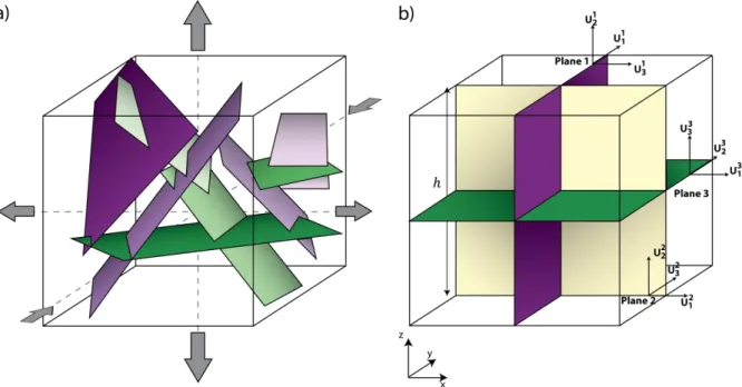
Now, let us consider a complex fractured medium embedded in an elementary volume at a certain depth (Fig. 1a). The surface deformation is the resultant of the slip (or opening) of all single fracture forming the complex unit. Looking for the best fit of slip, opening, position and orientation parameters of all fractures by modelling the surface deformation is a non-linear problem and its solution is generally non-unique. Therefore, a linear form of the strain nucleus is the global strain tensor that sums up the contribution of all individual internal strain tensors. This model can be setup by the use of three orthogonal planes of fictitious dislocations at fixed position (the
centroid of the considered volume) and orientation. This model is equivalent to a complex source model of the deformation at the surface (Figure 1b). A similar relation, linking the mean of the amount of displacement over the area of the fracture to the sum of seismic moments (Aki, 1966) occurring during a period of time, was described by Brune (1971) and later used by Kostrov (1974).
To be representative of a complex medium, the size of the equivalent model must be small with respect to its depth. The surface deformation can be inverted using this equivalent model, allowing to retrieve a unique solution for the effective deformation in the three orthogonal planes.
Fig. 1 a) Sketch of a complex fractured medium (e.g. fracture network in reservoirs characterization) with principal directions
of deformation. b) Model of the effective unit built with three planar dislocations of edge ℎ and associated frame such that (𝑈11, 𝑈21, 𝑈31), (𝑈12, 𝑈22, 𝑈32) and (𝑈13, 𝑈23, 𝑈33) correspond to strike, dip and tensile dislocations for plane 1, 2 and 3 respectively.
In the far field, this model is parametrized to produce the same deformation as the model in a).
Surface displacement and tilt result from changes of the strain tensor at depth, under the hypothesis of small deformations. The equivalent model of the fractured medium is the combination of three orthogonal planar dislocations with fixed position and orientation to take advantage of the linear dependency with slip and tensile parameters. The approximation of a single strain tensor stands as long as the source is relatively small compared to its depth. We estimate that the ratio of the cube edge (ℎ) over the depth of the source (𝑧𝑠) should be smaller than 0.2. Above this value, the surface deformation pattern produced by the system of fractures significantly differs
from the one given by the equivalent strain tensor. The analytical solution for the surface and internal displacements, strains and tilts due to shear and tensile on rectangular faults in a semi-infinite elastic half space has been described by Okada (1992). The source is a planar facet characterized by its length (𝐿), width (𝑊), location (𝑥𝑠, 𝑦𝑠, 𝑧𝑠), orientation (dip, azimuth) and dislocation type (strike 𝑈1, dip 𝑈2 or tensile 𝑈3). The induced deformation is linear with dislocation 𝑈𝑗 and non-linear with all other parameters.
Geodetic techniques such as GNSS, InSAR, levelling and tiltmeters measure the surface deformation induced by such a source. We propose analytical equations only for a tiltmeter network (gradient of vertical displacement). Nevertheless, similar equations can be easily derived for other geodetic measurements. We will focus on the long-term monitoring of a reservoir using a network of tiltmeters. Using solutions given by (Okada, 1992), the tilt signal 𝑑𝑠
⃗⃗⃗⃗ measured by 𝑁 instruments in both X and Y horizontal directions, can be expressed as the linear combinations of the dislocation values 𝑈𝑖 with their associated deformation model vector 𝛼 𝑖 :
𝑑𝑠
⃗⃗⃗⃗ = ∑3𝑖=1𝑈𝑖𝛼 𝑖 (1)
where 𝑑⃗⃗⃗⃗ and 𝛼 𝑠 𝑖 are vectors of dimensions (2𝑁) and 𝛼 𝑖 correspond to the contribution of dislocation parameter i to the signal recorded by each instrument. In this study, we consider three orthogonal Okada’s planes of fixed dimension (we consider the edge ℎ of the plane so that ℎ = 𝑊 = 𝐿) and orientation arbitrarily chosen in the 𝑥𝑦𝑧 reference system to build the elementary volume (Figure 1b). Okada’s plane can be dipping at an arbitrary angle, and be orientated at any arbitrary azimuth angle but no plunge (angle between the upper edge of the plane and the free surface) is considered. Our model has a fixed orientation with only potential azimuth variations. In Nikkhoo et al. (2017), they address this lack of freedom by considering an extended rectangular dislocation with a full rotational degrees of freedom (i.e. characterizing the plunge).
The frame associated with each plane is represented in Figure 1, permitting the correspondence between dislocation types and the components of the strain tensor (Eq. 2). We associate to each plane a slip (strike or dip) in one direction and a tensile deformation (𝑈𝑖𝑗) representing the strain deformation (𝜺). Due to the static equilibrium of the source within the medium, the strain tensor is symmetrical:
( 𝑈31 𝑈11 𝑈13 𝑈23 𝑈32 𝑈22 𝑈12 𝑈21 𝑈33 ) =1 𝑎( 𝜀𝑥𝑥 𝜀𝑥𝑦 𝜀𝑥𝑧 𝜀𝑦𝑥 𝜀𝑦𝑦 𝜀𝑦𝑧 𝜀𝑧𝑥 𝜀𝑧𝑦 𝜀𝑧𝑧 ) = ( 𝑝1 𝑝2 𝑝3 𝑝2 𝑝4 𝑝5 𝑝3 𝑝5 𝑝6 ) (2)
where 𝑈𝑖𝑗 are the dislocation types for all three planes: the subscript 1 to 3 stands for strike, dip and tensile for plane 1 to 3 (Figure 1). Hence, the tilt signal produced by a strain tensor source made of three Okada’s planes is linear with respect to the 6 components of the strain tensor 𝑝𝑖 (the strain tensor being symmetrical):
𝑑𝑠
⃗⃗⃗⃗ = ∑6𝑖=1𝑝𝑖𝛼 𝑖 (3)
The strain tensor source is hence described by 6 characteristic patterns of deformation 𝛼 𝑖 associated to each source component whose amplitude depends on the strength of the deformation, represented by the amount of dislocation 𝑝𝑖. In the next section, we describe these patterns of deformation as being the sensitivity associated to each component of the strain tensor.
2.2 Sensitivity map
The source tilt signal produced by a strain tensor given by Eq. 3 is the sum of the product between each strain parameter 𝑝𝑖 and the associated deformation vector 𝛼 𝑖. These vectors represent the known spatial variability of the forward model. They depend on the network distribution relative to the source location, dimension and orientation. Thus, for a unit deformation of a strain source at a fixed depth and location, the values of ‖𝛼 ‖ show, for each component, the sensitivity of the tiltmeter to the deformation.
On Figure 2, we perform this general sensitivity analysis to the domain used for the synthetic application. To ease the interpretation, we choose to represent the sensitivity of each strain component 𝑠𝑖=
‖𝛼⃗⃗ 𝑖‖
‖𝛼⃗⃗ ‖𝑚𝑎𝑥 (𝑖 = 1,6 )
normalized by the maximum value of ‖𝛼 ‖ for all 𝑖. The scale of sensitivity to the deformation ranges between 0 to 1, from insensitive to totally sensitive areas (Figure 2). Mean values of sensitivities are estimated for each component, over the 10x10 km domain. The 𝜀𝑥𝑧, 𝜀𝑦𝑧and 𝜀𝑧𝑧 components present higher sensitivities with a mean value of 𝑠̅̅̅̅̅ = 𝑠𝜀𝑥𝑧 ̅̅̅̅̅ = 0.17 and 𝑠𝜀𝑦𝑧 ̅̅̅̅̅ = 0.32 compared to 𝜀𝜀𝑧𝑧 𝑥𝑥, 𝜀𝑥𝑦 and 𝜀𝑦𝑦 components (𝑠̅̅̅̅̅ = 𝑠𝜀𝑥𝑥 ̅̅̅̅̅ = 0.11 and 𝜀𝑦𝑦 𝑠𝜀𝑥𝑦
̅̅̅̅̅ = 0.10). Indeed, tiltmeters measure the horizontal variations of the vertical changes of the ground (𝑡 = −∇⃗⃗ 𝑢𝑧). This suggests that 𝜀𝑥𝑧, 𝜀𝑦𝑧 and 𝜀𝑧𝑧 components should always be better resolved through the optimization process regardless of the network design.
Fig. 2 Normalized sensitivity distributions for the 6 components of the strain tensor. The sensitivity is estimated using the norm of the vector 𝛼 for each component normalized by the maximum value of the norm. The color code indicates low sensitive areas in white and highly sensitive areas in black. The locations of the tiltmeters in the synthetic network (see section 4) are represented by black dots.
3. Parameters identification
We estimate both source and instrument parameters from tilt signals using a two-step approach, employing 1) a least-square inversion and 2) a uniqueness enforcement.
3.1 Model Parametrization
The input data is measured using an array of 𝑁 tiltmeters composed by 𝑇 monthly-discrete measurements associated to the variation of the strain tensor components at depth. Following Furst et al. (2019), we assume that the tilt signal 𝑑⃗⃗⃗⃗ (𝑡) (2𝑁×𝑇) is the sum of the signal produced by the source 𝑑𝑜 ⃗⃗⃗⃗ (𝑡) (2𝑁×𝑇), a time-linear 𝑠 instrumental drift 𝑑⃗⃗⃗⃗ (𝑡) = 𝑎 𝑡 (2𝑁×𝑇) (𝑎 is the drift rate vector of dimension 2𝑁) and coloured noise 𝑐𝑛𝑑 ⃗⃗⃗⃗ (𝑡) (2𝑁×𝑇) associated to the tiltmeters (Eq. 3). We assume that the tidal signal has been removed from the tilt signal.
This synthetic signal is then used in the inversion process as the observation input. Seeking for source (𝑝𝑖) and instrumental (𝑎 ) parameters, we parametrize the modelled tilt as the sum of a source signal evolving in time and a time-linear component standing for the drift component.
3.2 Step 1: Global optimization framework
Although the problem is presented with linear governing equations for the strain tensor model, we present the inverse problem in its nonlinear form and use a global optimization framework. This enables the inversion platform to easily account for complex forward models, like poroelasticity and elastoplasticity, or extend the identification strategy to source locations.
This study considers 2𝑁 instrumental parameters and 6𝑇 source parameters to be retrieved using time series of tilt data including 2𝑁 ∙ 𝑇 observations. The optimization parameters are initialized with no a priori information, providing a first model prediction to be compared with the observations. During this stage of initialization, we also estimate the deformation model vector 𝛼 𝑖 of a unit source for both components of each tiltmeter (using Okada, 1992). Then, the modelled signal estimated at each iteration is simply the product of the parameter 𝑝𝑖(𝑡) by the deformation vector 𝛼 𝑖, allowing for a significant gain in computational time. The comparison between observed and modelled data is made using the weighted squared error as cost function, integrated over time following the trapezoidal rule (Eq. 5 from Furst et al., 2019). The functional needs to converge below one (ideally to 0) for the optimization to be complete, i.e. reaching a set of admissible parameters explaining the observations within the data uncertainties. To reach this minimum, our inversion process is based on a recursive algorithm defining a multi-criteria global optimization, varying not only the parameters of the model, but also the initial guesses (Ivorra et al., 2013; Mohammadi & Pironneau, 2009). This ensures that a given set of optimal model parameters achieves the global minimum of the cost function.
At the end of the optimization, the parametrization of tilt data leads to a system of linear equations whose solutions are infinite combinations of these parameters producing the same signal (Furst et al., 2019):
𝑑𝑎
⃗⃗⃗⃗ (𝑡) = ∑6𝑖=1𝛼 𝑖𝑝𝑖𝑎(𝑡)+ 𝑎⃗⃗⃗⃗ 𝑡 = ∑𝑎 6𝑖=1𝛼 𝑖𝑝𝑖∗(𝑡)+ 𝑎⃗⃗⃗⃗ 𝑡 ∗ (4) The subscript a represents any of all admissible sets including the best solution we reach with respect to the data
uncertainties (expressed by the exponent *), hereafter referred to as the target solution.
3.3 Step 2: Uniqueness enforcement
This set of admissible source and instrumental parameters (𝑝𝑖𝑎(𝑡) and 𝑎⃗⃗⃗⃗ ) is not unique since an infinite number 𝑎 of combinations of these parameters leads to the same value of the functional (Furst et al., 2019). This implies that
the solution of the optimization process can notably diverge from the target solution. The latter can be recovered from the admissible solution (Eq. 4) as,
𝑎∗ ⃗⃗⃗⃗ = 𝑎⃗⃗⃗⃗ − ∑𝑎 6𝑖=1𝛼 𝑖𝑅𝑖 , (5a) with, 𝑅𝑖= p𝑖∗−𝑝𝑖𝑎 𝑡 (5b)
where 𝑅𝑖 are the correction coefficients associated with each component of the strain tensor. Following Furst et al. (2019), we assume that the position of the instrument relatively to the source is not correlated to the drift rate components. Hence, the distributions of α⃗⃗ 𝑖 and 𝑎 must be statistically independent for each component of the strain tensor, that is 𝑐𝑜𝑣(𝑎⃗⃗⃗⃗ , 𝛼 ∗
𝑖) = 0. Introducing Eq. 5a in the latter equation leads to
𝑐𝑜𝑣(𝑎⃗⃗⃗⃗ , α𝑎 ⃗⃗ 𝑖) − ∑𝑘=16 𝑅𝑘𝑐𝑜𝑣(𝛼⃗⃗⃗⃗ , α𝑘 ⃗⃗ i) = 0 (6a) that we rewrite in matrix form,
𝐶 − 𝑅⃗ 𝑩 = 0 (6b)
The coefficients 𝑅⃗ can be inferred from Eq. 6b if the square matrix 𝑩 = 𝑐𝑜𝑣(𝛼⃗⃗⃗⃗ , 𝛼𝑘 ⃗⃗⃗ ) is invertible (det (𝑩) must be 𝑖 different from 0). We normalized matrix 𝑩 by its Frobenius norm to evaluate the determinant of the matrix. In our study, 𝑩 is invertible but this property should be checked for new instrumental distribution. This allows us to determine the coefficients 𝑅⃗ such as:
𝑅⃗ = 𝑩−1𝐶 (7)
The uniqueness enforcement produces six independent values 𝑅𝑘 which depend on the covariance matrix between admissible drift and deformation model vector, but also involve the covariance between the components of the deformation model vector. In Furst et al. (2019), 𝑅 coefficients corresponds to the linear regression between the drift rates and the components of the deformation model vector. Here, 𝑅𝑘 also involves the covariance matrix (𝑩) between the components of the deformation model vector, and therefore they depend on all 𝛼 𝑖 associated with each component of the strain tensor. This implies that the distribution of 𝑎⃗⃗⃗⃗ as a function of 𝛼 𝑎 𝑖, would not present a clear linear trend.
Incorporating 𝑅𝑘 into Eq. 5a and 5b provides us with a new admissible set of parameters (target solution) which should be closer to the exact solution without altering the residuals between observed and modeled data. Nevertheless, the target solution does not necessarily match the exact solution due to data uncertainties that are not captured by the model.
3.4 Parameters resolution analysis
We account for the data uncertainties in the inversion process by using the weighted Euclidian norm in 𝐽. Data uncertainties propagate through the inversion process to the parameters so that our target solution is the best guess with respect to the resolution of the data. For linear problems, we can directly estimate the resolution matrix associated with the least-square inversion process. Nevertheless, we propose a generic approach to estimate the parameter resolution, regardless of the linearity of the problem. We attempt to estimate ranges of confidence for each component of the strain tensor by adding small perturbations on the data. The mathematical development to obtain this parameter resolution analysis is detailed in Appendix A. This leads to two confidence intervals of the parameters: an instantaneous resolution 𝑃⃗⃗⃗⃗⃗ that only depends on data residuals, and a long-term resolution 𝑃𝐼𝑇 ⃗⃗⃗⃗⃗⃗ 𝐿𝑇 linked to a priori range of perturbations on the drift rates (see Appendix A for description of drift rates perturbations choice).
3.5 Algorithm
The following guideline summarizes the implementation of the method:
1. Tilt time series. The observed data are corrected from the tidal effect or any other known effects that may obscure the effect we are interested in.
2. Time intervals. Data are discretized in a user-defined number of epochs. This also defines the number of different source parameters that are sought.
3. Initialization. User defines the number of strain sources. For each one, a certain number of model parameters are fixed (𝑥𝑠, 𝑦𝑠, 𝑧𝑠, 𝑊, 𝐿). Research intervals are given for free parameters (𝑝𝑖(𝑡)) of each source and for instrumental parameters (𝑎 ). The source model vector 𝛼 𝑖 is calculated during the initialization.
4. Step 1: Inversion.
4.1. Forward model. A set of modelled data is obtained using the parameters associated to the strain tensor model.
4.2. Functional. Computation of the cost function 𝐽.
4.3. Optimization. While 𝐽 ≤ 𝜖 (𝜖 is user defined), the solver defines new values of free parameters for the forward model (4.1).
4.4. Admissible solution. Inversion gives a set of admissible solutions for 𝑝𝑖∗(𝑡) and 𝑎⃗⃗⃗⃗ . ∗ 5. Step 2: Uniqueness enforcement.
5.2. Target solution. Admissible solution is corrected using Eq. 5a and 5b producing the target solution. In the next section, we apply this algorithm to a synthetic case of a strain source deforming at depth.
4. Application to synthetic data 4.1 Model parametrization
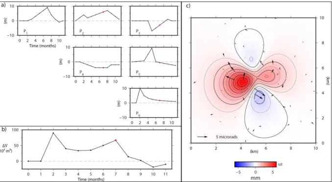
The two-step optimization approach generalized from Furst et al. (2019) provides unique and constrained parameters in linearly dependent forward models. We create the synthetic dataset from a single strain source (three Okada’s planes) deforming at depth. We assume a continuous deformation during 11 months split into 12 1-month intervals (initial step of the model is considered at 𝑡 = 0, final step at 𝑡 = 11 months), so we have 12 steps of the strain model to be characterized. The strain source is expressed in the reference frame made of three orthogonal planes of 100 m side embedded in an elastic medium at 1500 m depth, at the center of a 10x10 km domain. We choose random and independent time steps for each component of the strain tensor (black curves in Figure 3a-b), producing a complex surface signal. In Figure 3c, we represent one state (𝑡 = 7 months) of the vertical deformation (color scale) and synthetic tilts (black arrows) associated with the values of strain tensor components. The total volume variation at depth (Figure 3b) is estimated using the trace of the strain tensor,
Δ𝑉𝑖𝑛𝑗𝑒𝑐𝑡𝑖𝑜𝑛= (𝑝1+ 𝑝4+ 𝑝6)ℎ2 (8)
Besides the signal of the source, a time-dependent linear drift and a Brownian noise are included in the synthetic tilt signal. The drift components are randomly chosen using a uniform probability density function. The range of probability for drift rates is set to ±2.4 µrad/yr, corresponding to low drifting tiltmeters (Chawah et al., 2015; Furst et al., 2019). The Brownian noise is arbitrarily generated by accumulating random values within a standard deviation, depending on the time of the experiment. The initial standard deviation fixed using the short-term resolution of tiltmeters 𝜎𝑠ℎ𝑜𝑟𝑡=5 nrad grows towards a maximum standard deviation 𝜎𝑚𝑎𝑥=180 nrad at the end of the experiment. In our synthetic measurements, the covariance matrix is diagonal and uniformly set to the final value of standard deviation 𝜎𝑚𝑎𝑥 for all data. The noise signal is significantly smaller than the drift signal but it can affect both the instantaneous and long term trend in the tilt signal. Indeed, the linear component of Brownian noise can be superimposed to the linear instrumental drift. As a result, the optimization estimates the sum of both linear signals and interprets the value as the linear drift only.
The synthetic deformation induced by the strain source is monitored using an array of 50 tiltmeters randomly distributed (Figure 3c, Furst et al. (2019)). From Figure 2, we can see that this network is not optimized to capture at best all 6 components of the strain tensor since less than half the instruments are located in sensitive areas.
Continuous tilt data are downsampled to monthly time-interval measurements to decrease the number of parameters to infer, leading to 72 strain parameters and 100 drift parameters for 1200 tilt observations. In Figure 3c, we represent the vertical displacement of the surface at 𝑡 =7 months. The components of the strain tensor are indicated by red dots in Figure 3a, and the associated total volume variation is of 66 667 cubic meters (red dot in Fig 3b).
Fig. 3 a) Evolution of the six components of the strain tensor (𝜀𝑥𝑥, 𝜀𝑥𝑦, 𝜀𝑥𝑧, 𝜀𝑦𝑦, 𝜀𝑦𝑧, 𝜀𝑧𝑧) for an anisotropic (black curve) strain
source. b) Evolution of the total source volume variations (Eq. 8) for the 11 months of experiment. c) Vertical deformation (color scale) and synthetic tilts (black arrows) produced by an anisotropic strain source observed at the surface at 𝑡 =7 months (red dot on a and b).
4.2 Results
To retrieve the 6 parameters of the strain tensor, we invert the synthetic tilt dataset using the two-step optimization. Once the inversion of tilt data has converged, we obtain a set of optimal parameters including components of strain tensor and drift rates given by the tilt residuals. This admissible solution needs to be corrected using the correction coefficient to restore uniqueness. We hereafter describe the results of the two-step optimization in terms of tilt
residuals, drift rates parameters and strain tensor components. We complement the strain tensor components with instantaneous resolutions and long-term ranges of confidence as previously described.
4.2.1 Residual tilt signal
The best fit model produces a dataset giving the lowest residual between synthetic and modelled data. The data residuals are determined using the norm of the difference between modelled and observed tilt vector for each instrument and can be estimated at 3 different scales: 1) at data point scale, 2) at time-step scale and 3) at experiment scale. Figure 4a plots these residuals (crosses) as a function of time-steps. The inversion process provides a fairly homogeneous tilt residual over time for the whole set of tiltmeters (Figure 4a). Figure 4b displays the spatial distribution of data residuals at time 𝑡 = 7 months (blue crosses on Figure 4a). By averaging the residuals of all data points at a given time, we obtain a global residual for the considered time interval (red crosses on Figure 4a). Finally, we integrate the time-interval residuals over the entire experiment to get a mean global residual (green line on Figure 4a).
Fig. 4 a) Time distribution of the norm of tilt residuals for all data points (crosses). Red crosses indicate the averaged residual
for each time interval, blue crosses correspond to residuals displayed in b) and the green line displays the mean experiment residual. b) Spatial distribution of the tilt residual vectors at 𝑡 = 7 month (black arrows). The source is located by the orange square at the center of the domain.
Time-interval residuals range from 0.007 to 0.024 µrad with an average experiment residual of 0.010 µrad (green line on Figure 4a). Compared to the tilt uncertainty of 0.18 µrad, the residuals are significantly smaller. This is probably due to the parametrization of the tilt data, as being the sum of source and time-linear signals. Hence, the optimization tends to estimate all linear trends which may be present in the tilt signal, including drift rates and any noise that would be linear in time.
4.2.2 Drift rates
This admissible solution given by the first step of the optimization process belongs to a family of solutions described by Eq. 4. In Figure 5a and b, we plot the elements of 𝑎 (𝑥 and 𝑦 components) as a function of 𝛼⃗⃗⃗⃗⃗⃗ 𝑧𝑧 associated to the 𝜀𝑧𝑧-component of the strain tensor (Figure 5b being an enlargement of the grey area of Figure 5a). We choose to represent and describe only one component of the strain tensor where blue dots stand for admissible drift rates after the inversion, red inverted triangles for the corrected values and black crosses for the true synthetic values.
Before the uniqueness enforcement, the distribution of the drift rates was between bounds (given by tiltmeter manufacturers) resulting from the first step of the optimization. One can identify a trend between elements of 𝛼 and elements of 𝑎 inducing some correlation between the drift rates and the position of the instrument relatively to the source (blue line). In Furst et al. (2019), the correction is based on removing this correlation. In this study, the same process (that is, without taking into account the cross correlation between drift rates and model deformation vector) produces the distribution of drift rates (green diamonds), which is far from the true distribution of drift rates (black crosses). Here we use a coupled coefficient described by Eq. 7 to correct the optimal drift rates leading to values of drift rates (red inverted triangles) almost perfectly retrieved (black crosses).
Fig. 5 a) Relation between all components (x and y components) of drift rates 𝑎⃗⃗⃗⃗ and model coefficient 𝛼𝑎 ⃗⃗⃗⃗⃗⃗ associated to the 𝑧𝑧
𝜀𝑧𝑧 component of the strain tensor. Black crosses represent the true synthetic solution. After the first step of optimization, the
admissible solution given by the blue dots shows a correlation (blue line). Correcting only this correlation leads to a distribution (green diamonds) largely dependent on the components of 𝛼⃗⃗⃗⃗⃗⃗ . In addition to this correlation coefficient, the correction involves 𝑧𝑧
the covariance of the components of 𝛼 as provided by Eq. 7. The resulting distribution of 𝑎⃗⃗⃗⃗ (red inverted triangles) is totally ∗
uncorrelated with elements of 𝛼 associated to all six components of the strain tensor. b) Enlargement of the grey rectangle in
4.2.3 Strain tensor components and volume variations
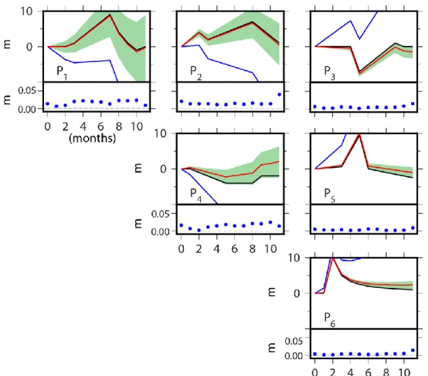
Along with the drift rates, the inversion produces admissible variations of strain tensor components 𝑝𝑖𝑎 (blue line in Figure 6) depending on the tilt residuals. The shape of each component variation is preserved compared with the target history (black line in Figure 6), but a strong linear trend persists due to non-uniqueness of the solution. We interpret this linear trend as the consequence of incorrect estimation of the instrumental drifts. Admissible solutions 𝑝𝑖𝑎 are corrected using the coupled coefficients 𝑅𝑖 in Eq. 5b to obtain the target solutions 𝑝∗ (red line in Figure 6). For all components, the uniqueness enforcement largely improves the solution. For instance, a slight linear trend remains in 𝜀𝑦𝑦 while 𝜀𝑥𝑥 and 𝜀𝑥𝑦 are almost perfectly restored.
While we demonstrate the efficiency of our strategy on synthetic data, the target solution is not available when using real case datasets. As a result, we complement these target solutions 𝑝∗ with two resolution analyses: one considering each time-step separately 𝑃⃗⃗⃗⃗⃗ and a second one involving the entire time series 𝑃𝐼𝑇 ⃗⃗⃗⃗⃗⃗ . The instantaneous 𝐿𝑇 resolution is determined using the tilt residuals for each component of a tiltmeter at a given time. The residuals associated to each tilt component of the experiment range between 0 and 0.08 µrad (Figure 4a), which is largely lower than the Brownian noise generated in the synthetic. We assume that the level of resolution of the tilt in the inversion depends on the parametrization of the tilt data. Therefore, the instantaneous resolution (Eq. A.3, blue dots in graphs below each parameter variations on Figure 6) is 2 orders of magnitude lower than the parameters. In Figure 6, we only represent the positive instantaneous resolution (the negative bound being the symmetric). One can notice that the instantaneous resolution is higher for 𝜀𝑥𝑧, 𝜀𝑦𝑧 and 𝜀𝑧𝑧 than for 𝜀𝑥𝑥, 𝜀𝑥𝑦 and 𝜀𝑦𝑦. This difference lies in the matrix 𝑨, which contains the deformation model vectors associated to each instrument for all of the strain tensor components. 𝜀𝑥𝑧, 𝜀𝑦𝑧 and 𝜀𝑧𝑧 components show high sensitivity compared to the three other components (Figure 2), resulting in almost constant instantaneous resolution for 𝜀𝑥𝑧, 𝜀𝑦𝑧 and 𝜀𝑧𝑧 and more variable instantaneous resolution for 𝜀𝑥𝑥, 𝜀𝑥𝑦 and 𝜀𝑦𝑦 components.
The long-term resolution is built using a constraint on the drift rates (user defined, see Appendix A) and increases with time. As part of the optimization parameters, the drift rate distribution is defined by its dispersion around a mean value of 0 (i.e. its standard deviation) and by the gradient of the functional for each drift parameter (Eq. A.4). Hence, 𝑃⃗⃗⃗⃗⃗⃗ depends on inaccuracy in the minimization of the functional and on the quality of the tiltmeters. Indeed, 𝐿𝑇 highly drifting instruments would present a high standard deviation, increasing the range of sensitivity. Perturbations of the drift rates impact all components of the strain tensor in the same way but 𝑃⃗⃗⃗⃗⃗⃗ also depends on 𝐿𝑇 the tilt network through matrix 𝑨 similarly to 𝑃⃗⃗⃗⃗⃗ . Therefore, the range of sensitivity is different for each 𝐼𝑇 component as shown in Figure 6 (green area). In our study, the resolution matrix is close to the identity, meaning
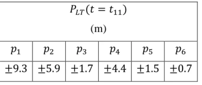
that the tilt network is not blind to any component of the deformation at depth. All confidence intervals include the target solution but as expected from the sensitivity map. 𝜀𝑥𝑥, 𝜀𝑥𝑦 and 𝜀𝑦𝑦 components present a wide range of resolution contrarily to that of 𝜀𝑥𝑧, 𝜀𝑦𝑧 and 𝜀𝑧𝑧. The values of at the end of the experiment, 𝑃⃗⃗⃗⃗⃗⃗ for the 6 𝐿𝑇 components of the strain tensor are given in Table 1. Optimizing the spatial distribution of the tilt network improves the target solution and the range of resolution, but 𝜀𝑥𝑧, 𝜀𝑦𝑧 and 𝜀𝑧𝑧 components will always present a better range of resolution than the other components.
𝑃
𝐿𝑇(𝑡 = 𝑡
11)
(m)
𝑝
1𝑝
2𝑝
3𝑝
4𝑝
5𝑝
6±9.3 ±5.9 ±1.7 ±4.4 ±1.5 ±0.7
Fig. 6 Evolution of the 6-strain tensor components over time. For each component, we represent in the upper graphs, the
long-term evolutions and resolutions, and in the lower graph using blue dots, the upper bound of the instantaneous resolution 𝑃⃗⃗⃗⃗⃗ . 𝐼𝑇
The target values are indicated by the black line, the admissible solution 𝑝𝑖𝑎 from the inversion by the blue line and the target
solution 𝑝𝑖∗ from the correction by the red line. Ranges of long-term sensitivity, 𝑃 𝐿𝑇
⃗⃗⃗⃗⃗⃗ (green areas) bound the corrected solution for each component.
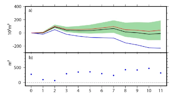
From the components of the strain tensor, we can derive the history of volume variations defined by Eq. 8 and represented in Figure 7a. Instantaneous and long-term resolutions can also be estimated using the same relation as Eq. 8 and involving 𝑃⃗⃗⃗⃗⃗ and 𝑃𝐼𝑇 ⃗⃗⃗⃗⃗⃗ associated to 𝜀𝐿𝑇 𝑥𝑥, 𝜀𝑦𝑦 and 𝜀𝑧𝑧 components. Figure 7a shows the target volume as a black line, the admissible volume as a blue line and the corrected volume as a red line within a range of sensitivity
in green. Because the long-term resolution of each diagonal component is added, the range of sensitivity is wide. Figure 7b represent the instantaneous resolution of the volume variation reaching a maximum of ±490 m3 at 𝑡 =
11.
Fig. 7 a) Evolution of the volume variation over time. The black line represents the target volume history, the blue one is the
admissible volume variation and the red line is the corrected volume variation. The green area indicates the long-term resolution of the volume variation associated with the red line. b) Representation of the upper bound of the instantaneous resolution for the volume variation.
5. Discussion
In this study, we present a concept, based on standard Okada’s model, for describing deep complex fracture sources. Under the assumption that the source size is small compared to its depth, we state that a strain tensor model captures the sum of all tensile, dip and strike-slip fracture motion. Therefore, the surface motion associated to the strain tensor is equivalent to the one produced by the fracture network. This strain tensor is an effective image, characterized by six parameters, which intrinsically reflects the fracture network constituting the considered volume. Associated to the strain components, patterns of deformation describe the sensitivity of tiltmeters to the deformation. The sensitivity analysis highlights that all components of the strain tensor cannot be solved equally well. This is probably due to the limited capability of tilt data (2-D) to characterize all components of the strain tensor (3-D entity). As tiltmeters are more sensitive to the vertical displacement of the source, the strain components involving horizontal motion are poorly determined. To overcome the problem, the use of other
geodetic measurements sensitive to horizontal displacement of the surface, such as 3-D GNSS data or strainmeters may improve the estimation and resolution of the 𝜺𝒙𝒙, 𝜺𝒙𝒚 and 𝜺𝒚𝒚 components. Such a network design is conceivable for oil and gas exploitations but also for some volcanoes where the monitoring involves a wide range of geodetic network.
A major advantage of our approach is to use a well-posed inverse problem. Indeed, the two-step methodology developed in the paper allows to retrieve the unique solution of the strain tensor using surface tilt data (or any other geodetic measurements). However, the issue remains to associate the parameters of the global strain tensor with the individual tensile and slip motions of a fracture set. Without any complementary information, the strain tensor can only be analyzed in terms of principal values and directions of the volume. To determine orientation and internal slip motions associated with fracture families constituting the volume, the use of external information is necessary like geological studies, seismic events (in volcanic systems) and microseismicity (in geothermal, mining and oil and gas exploitations). This a priori information permits to characterize active fracture or fault planes in terms of position and geometry, and the question is whether or not their dynamic can be obtained using the strain tensor.
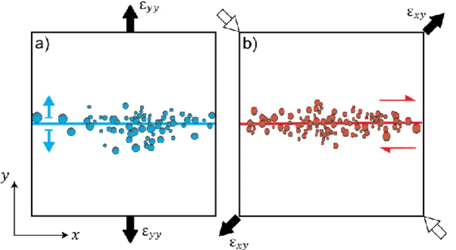
In oil and gas exploitations, the injection of fluid in a tight reservoir produces a nanometric scale deformation along with a microseismic signal typically aligned to form a fracture. With fracture positions and orientations determined through microseismicity (e.g. Wessels et al., 2011), we can infer the type (tensile, strike or dip) and amplitude of slip motion. Figure 8 illustrates schematic examples of 2-D fractured domains characterized by microseismicity (blue and red dots) with strain tensors (black and with arrows) resulting from the optimization approach. For each case, the strain tensor can be interpreted using a priori knowledge about position and orientation of the fractures, leading to slip motions of the fractures (tensile for Figure 8a and strike slip for Figure 8b). To do so, we solve a system of linear equations. In 2-D the model considers 1 Okada’s plane having an infinite width. This system includes 3 equations (number of independent strain parameters) and two unknowns defined by the types of slip associated to each fracture family. When only one fracture family is considered (Figure 8a-b), the solution is overdetermined. However, this overdetermined system should have solutions because of fracture configuration: tensile motion can only occur in the orthogonal direction of the fracture plane. Hence, the associated system should contain only two equations (𝜺𝒙𝒙 or 𝜺𝒚𝒚= 𝟎) for two unknowns. On the other hand, if the system truly includes three independent equations, this implies that several fracture families are involved, leading to an under-determined problem. In such a case, more assumptions (e. g. fixing type of slip motion) need to be made to discriminate between the solutions. Similarly, in 3-D (3 Okada’s planes) the system of equations is defined by the six independent parameters of the strain tensor, while the equivalent fracture model has three unknowns (tensile,
strike and dip-slip). Hence, types and amplitudes of slip motions can be fully determined if two fracture families have been identified. The general case involving all slips of a fracture family need to be defined as an inverse problem with additional constraints such as the strength and friction of the fractures, in order to reduce its intrinsic non-uniqueness. This approach seems to be feasible by using the methods developed by Angelier (1984), Angelier et al. (1982) and by Etchecopar (1984) for fault slip and stress inversion.
Fig. 8 Schematic representation of two fractured domains in 2-D. Blue and red circles represent microseismic events defining
fracking planes (blue and red line). a) The strain tensor given by the inversion is represented by black arrows around the elementary volume. Knowing the geometry and orientation of the fracture (blue line), the strain tensor is interpreted as an opening along the fracture plane (blue arrows). b) Considering fracture orientation from a priori knowledge (red line), the strain tensor represented by black and white arrows around the elementary volume can be interpreted as a strike slip (red arrows).
This model of strain tensor can be used to characterize complex fracture networks occurring in hydraulic fracturing in mining, geothermal or oil and gas extraction. Indeed, the injection of material at depth along kilometric scale horizontal wells, generates fractures in addition to natural fracking, creating networks with various fracture orientations. Therefore, during the exploitation of the reservoir, these fractures may behave differently depending on the applied stress. Thanks to the full strain tensor model, we can estimate from the surface data the state of the deformation at depth. The strain tensor would allow the identification of preferential deep movements, leading to families of fractures or faults that have played to produce the surface signal. In the specific case of oil exploitation, this would improve monitoring of exploitations by identifying potential pre-existing fractures or faults at depth, that are reactivated during injection or extraction. Furthermore, modelling the deformation of a superficial source requires to consider a collection of strain tensors to respect the far field equivalence. Hence, an efficient
of production but also temporal and spatial strain orientations. Finally, the use of the strain tensor model in volcanic systems would provide information on deformation of the magma chamber or magma movements in dikes or sills, and potentially identify anisotropic deformation of the various sources.
6. Conclusion
In this study, we address the issue of monitoring and characterizing complex fracture reservoirs. Such reservoirs are common in mining, oil or gas exploitations and need a careful monitoring scheme to optimize the production and to follow the induced deformation. Even if the individual characteristics of such complex sources cannot be uniquely determined from surface deformation using a classical analytical source, the deformation of a complex fracture network still results in a unique surface deformation. When the source considered is significantly small with respect to its depth, we can express the deep deformation in a new basis to obtain the global effective deformation of the medium. The choice made here for this basis is three mutually orthogonal Okada’s dislocations. The resulting strain tensor of the deep source produces the same far field signal as the true complex medium. We develop a source model of fixed position, dimensions and orientation that can represent various amplitude of shear and tensile deformations at depth. By doing so, we reduce a complex non-linear problem to a linear problem with a unique solution between the surface deformation and the source signal. We adapt the two-step methodology developed in Furst et al. (2019) to infer the source and instrumental parameters from tilt signal at the surface. The linearity of the strain tensor model significantly reduces the computational cost when inverting tilt data (or any other geodetic measurements).
The synthetic study shows the strong dependence of the instrument location with respect to the source and the sensitivity of the instrument. In particular, tiltmeters measure the gradient of the vertical displacement and are therefore more sensitive to the z-component of the strain tensor than to purely horizontal components. The confidence intervals illustrate this dependency with a better resolution for 𝜀𝑥𝑧, 𝜀𝑦𝑧 and 𝜀𝑧𝑧 components than for 𝜀𝑥𝑥-, 𝜀𝑥𝑦- and 𝜀𝑦𝑦-components. Complementing the tiltmeter network with additional geodetic data, such as GNSS or strainmeters network, could bring a better resolution of the parameters in the horizontal components.
Implemented on real datasets, the unique solution from the tilt data inversion can be interpreted using the principal directions of the tensor, leading to main deformations of the complex fracture network. Using available geology of the subsurface structures, we could identify families of fractures producing the surface deformation and report any reactivation of faults or fractures.
Author contribution statement
J.C. devised the main conceptual ideas. S.F. and M.P. developed the theory and B.M. worked out the global algorithm. S.F. designed and performed the numerical calculations for the experiments. J.C., B.M. and M.P. supervised the findings of this work. S.F. wrote the manuscript and designed the figures with support from M.P., J.C. and B.M. All authors provided critical feedback and discussed the results.
Data availability statement
The synthetic datasets generated and analysed during the current study are available on request from the corresponding author.
Acknowledgments
The post-doctoral research project of S. Furst was fully supported by the Total Company. We thank Maurizio Battaglia, Gábor Papp and an anonymous reviewer for their advice and suggestions, which improved the quality, value and clarity of the paper. We also thank Megan Cook for her careful proofreading of this paper.
Appendix A: parameters resolution analysis
The approach leading to parameter resolution analysis (Tarantola, 2004) can be extended to a generic formulation. Considering small perturbations, Eq. 4 gives:
𝑑𝑠 (𝑡) = ∑6𝑖=1𝛼 𝑖 (𝑑𝑝𝑖)(𝑡)+ (𝑑𝑎 ) 𝑡 (A.1)
Eq. A.1 leads to 2𝑁 equations for both 𝑥 and 𝑦 components of tilt data and instrumental drift and can be rewritten as:
𝑆 = 𝑨 𝑃⃗ + 𝐷⃗⃗ 𝑡 (A.2)
where 𝑆 (2𝑁) and 𝑃⃗ (6) are vectors of source signal and strain parameter perturbations at a given time, 𝐷⃗⃗ (2𝑁) are perturbations on the drift rates parameters and 𝑨 (2𝑁, 6) includes all components of the deformation model vector. To assess the parameter resolution 𝑃⃗ , we invert the matrix 𝑨 using a least-square method. Using Eq. A.2, we define the confidence intervals of the parameters 𝑃⃗ as the sum of an instantaneous resolution, 𝑃⃗⃗⃗⃗⃗ = (𝑨𝐼𝑇 𝑡𝑨)−1𝑨𝑡𝑆 and a long-term one 𝑃⃗⃗⃗⃗⃗⃗ = (𝑨𝐿𝑇 𝑡𝑨)−1𝑨𝑡(−𝐷⃗⃗ 𝑡):
Both resolutions depend on matrix 𝑨 which means that they are influenced by the position of the tiltmeter network relatively to the source and by the physics of the source itself (i.e. the type of model used, here the strain tensor). Instruments placed in sensitive areas should improve determination of the parameter and consequently narrow the confidence interval. The difference between the two resolutions lies in the perturbation component: the short-term resolution 𝑃⃗⃗⃗⃗⃗ depends on the perturbation of tilt data 𝑆 while the long-term resolution 𝑃𝐼𝑇 ⃗⃗⃗⃗⃗⃗ is influenced by 𝐿𝑇 perturbations on the drift rates 𝐷⃗⃗ and increases with time.
In this study, we set the perturbations on the data 𝑆 using the residual value for each component of the tilt signal, defined by the difference between optimal and observed signal. This residual is linked to both the coloured noise 𝑐𝑛
⃗⃗⃗⃗ and the probable lack of convergence of the inversion due to data uncertainties. Regarding drift rates perturbations 𝐷⃗⃗ , we only have drift values 𝑎𝑖∗ (𝑖 = 𝑥, 𝑦) from the optimization process and the gradient of the functional for each drift parameters 𝑑𝑗𝑖=
𝑑𝐽
𝑑𝑎𝑖 given by the inversion (at the optimum). Small values of gradients mean better resolved parameter 𝑎𝑖. We can estimate the dispersion associated to the optimal drift rate distribution through its associated standard deviation 𝜎𝑑. We choose to estimate the 𝑃⃗⃗⃗⃗⃗⃗ using a 2-𝜎𝐿𝑇 𝑑 uncertainty. However, this value being homogeneous for all drift parameters, we weight this standard deviation according to the gradient of the functional for the drift parameters such as
𝐷⃗⃗ = 2𝛾𝜎⃗⃗⃗⃗ 𝑑 (A.4)
where 𝜸 = 𝜺𝟏+ 𝜺𝟐
|𝒅𝒋𝒊|−𝒅𝒋𝒎𝒊𝒏
𝒅𝒋𝒎𝒂𝒙−𝒅𝒋𝒎𝒊𝒏, 𝜺𝟏 and 𝜺𝟐 being user defined. By doing so, we want to increase the uncertainty on
less resolved parameters. Returning to the interpretation of parameter resolutions, the short-term resolution 𝑷⃗⃗⃗⃗⃗⃗ , 𝑰𝑻 depends on the capacity of the inversion to converge towards an optimal and unique solution. Because tiltmeters present an excellent instantaneous resolution (up to 5 nrad), 𝑷⃗⃗⃗⃗⃗⃗ at a given time would be well retrieved. On the 𝑰𝑻 contrary, the long-term resolution 𝑷⃗⃗⃗⃗⃗⃗⃗ depends on errors on the drift rate estimation and increases with time. For 𝑳𝑻 highly drifting tiltmeters, the high value of variance (Furst et al., 2019) implies large ranges of confidence.
References
Aki, K. (1966). Generation and Propagation of G Waves from the Niigata Earthquake of June 16, 1964. Estimation of earthquake moment, released energy, and stress-strain drop from the G wave spectrum. Bulletin of the Earthquake Research Institute, 44, 73–88.
Alpala, J., Alpala, R., & Battaglia, M. (2017). Monitoring remote volcanoes: The 2010–2012 unrest at Sotará volcano (Colombia). Journal of Volcanology and Geothermal Research.
https://doi.org/10.1016/j.jvolgeores.2017.05.021
Angelier, J. (1984). Tectonic analysis of fault slip data sets. Journal of Geophysical Research. https://doi.org/10.1029/JB089iB07p05835
Angelier, J., Lybéris, N., Le Pichon, X., Barrier, E., & Huchon, P. (1982). The tectonic development of the hellenic arc and the sea of crete: A synthesis. Tectonophysics. https://doi.org/10.1016/0040-1951(82)90066-X Astakhov, D. K., Roadarmel, W. H., Nanayakkara, a S., & Service, H. (2012). SPE 151017 A New Method of
Characterizing the Stimulated Reservoir Volume Using Tiltmeter-Based Surface Microdeformation Measurements. In SPE Hydraulic Fracturing Technology Conference (pp. 1–15). The Woodlands, Texas. Bato, M. G., Pinel, V., & Yan, Y. (2017). Assimilation of Deformation Data for Eruption Forecasting: Potentiality
Assessment Based on Synthetic Cases. Frontiers in Earth Science, 5(June), 1–23. https://doi.org/10.3389/feart.2017.00048
Bonaccorso, A., Gambino, S., Guglielmino, F., Mattia, M., Puglisi, G., & Boschi, E. (2008). Stromboli 2007 eruption: Deflation modeling to infer shallow-intermediate plumbing system. Geophysical Research Letters, 35(6), 6–11. https://doi.org/10.1029/2007GL032921
Boudin, F., Bernard, P., Longuevergne, L., Florsch, N., Larmat, C., Courteille, C., Blum, P. A., Vincent, T. Kammentaler, M. (2008). A silica long base tiltmeter with high stability and resolution. Review of Scientific Instruments, 79(3), 1–11. https://doi.org/10.1063/1.2829989
Brune, J. N. (1971). Seismic Source, Fault-plane Studies, and Tectonics. In 15-th General Assembly IUGG. Van Camp, M., & Vauterin, P. (2005). Tsoft: Graphical and interactive software for the analysis of time series and
Earth tides. Computers and Geosciences, 31(5), 631–640. https://doi.org/10.1016/j.cageo.2004.11.015 Chawah, P., Chéry, J., Boudin, F., Cattoen, M., Seat, H. C., Plantier, G., Lizion, F., Sourice, A., Bernard, P.,
Brunet, C., Boyer, D., Gaffet, S. (2015). A simple pendulum borehole tiltmeter based on a triaxial optical-fibre displacement sensor. Geophysical Journal International, 203(2), 1026–1038. https://doi.org/10.1093/gji/ggv358
Chen, H. C., Kümpel, H., & Krawczyk, C. M. (2010). Field layout of a tiltmeter array to monitor micro-deformation induced by pumping through a horizontal collector well. Near Surface Geophysics, 8, 321–330. https://doi.org/10.3997/1873-0604.2010023
Davis, P. M. (1986). Surface Deformation Due to Inflation of an Arbitrarily Oriented Triaxial Ellipsoidal Cavity in an Elastic Half-Space, With Reference to Kilauea Volcano, Hawaii. Journal of Geophysical Research, 91, 7429–7438.
Dvorak, J. J., & Dzurizin, D. (1997). Volcano Geodesy: the search for magma reservoirs and the formation of eruptive vents. Reviews of Geophysics, 35(3), 343–384.
Dzurisin, D. (2006). Volcano Deformation. Volcano Deformation. https://doi.org/Doi 10.1007/978-3-540-49302-0
Etchecopar, A. (1984). Etude des états de contrainte en tectonique cassante et simulations de déformations plastiques: approche mathématique. Université de Montpellier II.
Furst, S., Chéry, J., Mohammadi, B., & Peyret, M. (2019). Joint estimation of tiltmeters drift and volume variation during reservoir monitoring. Journal of Geodesy. https://doi.org/10.1007/s00190-019-01231-3
Gambino, S., Falzone, G., Ferro, A., & Laudani, G. (2014). Volcanic processes detected by tiltmeters: A review of experience on Sicilian volcanoes. Journal of Volcanology and Geothermal Research, 271, 43–54. https://doi.org/10.1016/j.jvolgeores.2013.11.007
Honda, R., Yukutake, Y., Morita, Y., Sakai, S., Itadera, K., & Kokubo, K. (2018). Precursory tilt changes associated with a phreatic eruption of the Hakone volcano and the corresponding source model. Earth, Planets and Space. https://doi.org/10.1186/s40623-018-0887-4
Ivorra, B., Mohammadi, B., & Ramos, A. M. (2013). Design of code division multiple access filters based on sampled fiber Bragg grating by using global optimization algorithms. Optimization and Engineering, 1–19.
https://doi.org/10.1007/s11081-013-9212-z
Jahr, T., Letz, H., & Jentzsch, G. (2006). Monitoring fluid induced deformation of the earth’s crust: A large scale experiment at the KTB location/Germany. Journal of Geodynamics, 41(1–3), 190–197. https://doi.org/10.1016/j.jog.2005.08.003
Jahr, T., Jentzsch, G., Gebauer, A., & Lau, T. (2008). Deformation, seismicity, and fluids: Results of the 2004/2005 water injection experiment at the KTB/Germany. Journal of Geophysical Research: Solid Earth, 113(11), 1–10. https://doi.org/10.1029/2008JB005610
Kamo, K., & Ishihara, K. (1989). A Preliminary Experiment on Automated Judgement of the Stages of Eruptive Activity Using Tiltmeter Records at Sakurajima, Japan. Volcanic Hazards, 585–598. https://doi.org/10.1007/978-3-642-73759-6_35
Kostrov, V. V. (1974). Seismic moment and energy of earthquakes, and seismic flow of rock. Izv. Acad. Sci. USSR Phys. Solid Earth, 1(Eng. Transl), 23–40. https://doi.org/10.1016/0148-9062(76)90256-4
Maisons, C., Raucoules, D., & Carnec, C. (2006). Monitoring of slow ground deformation by satellite differential radar-interferometry . A reference case study . In Solution Mining Research Institute (pp. 1–10). Brussels. Masterlark, T. (2007). Magma intrusion and deformation predictions: Sensitivities to the Mogi assumptions.
Journal of Geophysical Research, 112(B6), B06419. https://doi.org/10.1029/2006JB004860
McTigue, D. F. (1987). Elastic stress and deformation near a finite spherical magma body: Resolution of the point source paradox. Journal of Geophysical Research, 92(B12), 12931–12940. https://doi.org/10.1029/JB092iB12p12931
Mohammadi, B., & Pironneau, O. (2009). Applied Shape Optimization for fluids (2nd Editio). Oxford: Oxford University Press.
Montgomery-Brown, E. K., Sinnett, D. K., Poland, M., Segall, P., Orr, T., Zebker, H., & Miklius, A. (2010). Geodetic evidence for en echelon dike emplacement and concurrent slow slip during the June 2007 intrusion and eruption at Klauea volcano, Hawaii. Journal of Geophysical Research: Solid Earth, 115(7), 1–15. https://doi.org/10.1029/2009JB006658
Narváez Medina, L., Arcos, D. F., & Battaglia, M. (2017). Twenty years (1990-2010) of geodetic monitoring of Galeras volcano (Colombia) from continuous tilt measurements. Journal of Volcanology and Geothermal Research, 344, 232–245. https://doi.org/10.1016/j.jvolgeores.2017.03.026
Nikkhoo, M., Walter, T. R., Lundgren, P. R., & Prats-Iraola, P. (2017). Compound dislocation models (CDMs) for volcano deformation analyses. Geophysical Journal International, 208(2), 877–894. https://doi.org/10.1093/gji/ggw427
Nishi, K., Hendrasto, M., Mulyana, I., Rosadi, U., & Purbawinata, M. A. (2007). Micro-tilt changes preceding summit explosions at Semeru volcano , Indonesia, 151–156.
Okada, Y. (1992). Internal deformation due to shear and tensile faults in a half-space. Bulletin of the Seismological Society of America, 82(2), 1018–1040.
Palano, M., Puglisi, G., & Gresta, S. (2008). Ground deformation patterns at Mt. Etna from 1993 to 2000 from joint use of InSAR and GPS techniques. Journal of Volcanology and Geothermal Research, 169(3–4), 99– 120. https://doi.org/10.1016/j.jvolgeores.2007.08.014
Peltier, A., Bachèlery, P., & Staudacher, T. (2011). Early detection of large eruptions at Piton de La Fournaise volcano (La Réunion Island): Contribution of a distant tiltmeter station. Journal of Volcanology and Geothermal Research, 199(1–2), 96–104. https://doi.org/10.1016/j.jvolgeores.2010.11.006
Poland, M. P., & Carbone, D. (2016). Insights into shallow magmatic processes at Kīlauea Volcano, Hawaiʻi, from a multiyear continuous gravity time series. Journal of Geophysical Research: Solid Earth, 121(7), 5477– 5492. https://doi.org/10.1002/2016JB013057
Segall, P. (2013). Volcano deformation and eruption forecasting. Geological Society, London, Special Publications, 380(1), 85–106. https://doi.org/10.1144/SP380.4
Tarantola, A. (2004). Inverse Problem Theory and Methods for Model Parameter Estimation. (SIAM, Ed.), Book. SIAM. https://doi.org/10.1137/1.9780898717921
Vasco, D. W., Ferretti, A., & Novali, F. (2008). Reservoir monitoring and characterization using satellite geodetic data: Interferometric synthetic aperture radar observations from the Krechba field, Algeria. Geophysics, 73(6), WA113. https://doi.org/10.1190/1.2981184
Verdon, J. P., Kendall, J.-M., Stork, A. L., Chadwick, R. A., White, D. J., & Bissell, R. C. (2013). Comparison of geomechanical deformation induced by megatonne-scale CO2 storage at Sleipner, Weyburn, and In Salah. Proceedings of the National Academy of Sciences, 110(30), E2762–E2771. https://doi.org/10.1073/pnas.1302156110
Warpinski, N. (2014). Surface Tiltmeters : A Proven Tool for New Answers in Unconventional Reservoir Stimulations.
Wessels, S. A., De La Pena, A., Kratz, M., Williams-Stroud, S., & Jbeili, T. (2011). Identifying faults and fractures in unconventional reservoirs through microseismic monitoring. First Break, 29(7), 99–104.
Zhou, J., Zeng, Y., Jiang, T., Zhang, B., & Zhang, X. (2015). Tiltmeter Hydraulic Fracturing Mapping on a Cluster of Horizontal Wells in a Tight Gas Reservoir. In SPE/IATMI Asia Pacific Oil & Gas Conference and Exhibition. Bali, Indonesia.