HAL Id: hal-02864168
https://hal.archives-ouvertes.fr/hal-02864168
Submitted on 10 Jun 2020
HAL is a multi-disciplinary open access
archive for the deposit and dissemination of
sci-entific research documents, whether they are
pub-lished or not. The documents may come from
teaching and research institutions in France or
abroad, or from public or private research centers.
L’archive ouverte pluridisciplinaire HAL, est
destinée au dépôt et à la diffusion de documents
scientifiques de niveau recherche, publiés ou non,
émanant des établissements d’enseignement et de
recherche français ou étrangers, des laboratoires
publics ou privés.
To cite this version:
Tom Gillooly, Nicolas Coltice, Christian Wolf. An Anticipation Experiment for Plate Tectonics.
Tectonics, American Geophysical Union (AGU), 2019, �10.1029/2018TC005427�. �hal-02864168�
1Université de Lyon, INSA-Lyon, CITI-Lab, INRIA-Chroma, France,2Laboratoire de Géologie, Ecole normale supérieure/CNRS UMR8538, PSL Research University, Paris, France,3LIRIS UMR CNRS 5205, France
Abstract
Although plate tectonics has pushed the frontiers of geosciences in the past 50 years, it has legitimate limitations, and among them we focus on both the absence of dynamics in the theory and the difficulty of reconstructing tectonics when data are sparse. In this manuscript, we propose an anticipation experiment, proposing a singular outlook on plate tectonics in the digital era. We hypothesize that mantle convection models producing self-consistently plate-like behavior will capture the essence of theself-organization of plate boundaries. Such models exist today in a preliminary fashion, and we use them here to build a database of mid-ocean ridge and trench configurations. To extract knowledge from it, we develop a machine learning framework based on Generative Adversarial Networks (GANs) that learns the regularities of the self-organization in order to fill gaps of observations when working on reconstructing a plate configuration. The user provides the distribution of known ridges and trenches, the location of the region where observations lack, and our digital architecture proposes a horizontal divergence map from which missing plate boundaries are extracted. Our framework is able to prolongate and interpolate plate boundaries within an unresolved region but fails to retrieve a plate boundary that would be completely contained inside of it. The attempt we make is certainly too early because geodynamic models need improvement and a larger amount of geodynamic model outputs, as independent as possible, is required. However, this work suggests applying such an approach to expand the capabilities of plate tectonics is within reach.
1. Introduction
For the past 50 years, the Earth science community has tried to expand the limits of plate tectonics theory. The simplicity of its essence, rigid blocks moving on a sphere (Morgan, 1968), allowed rapid progress in reconstructing the motion of the Earth surface. Plate reconstructions have stretched out their potential to deeper times (Domeier & Torsvik, 2014; Young et al., 2019) and connected to other global scientific questions, like carbon cycling (Pall et al., 2018). But the intrinsic limitations of plate tectonics still persist today. They are (a) dependent on seafloor data, which makes uncertainties of plate reconstructions beyond 50 Ma difficult to realize with accuracy; (b) more complex types of plate boundaries are needed; and (c) plates are not completely rigid, especially in the interesting places for geologists (mountains, rifts, and pull-apart basins). To go beyond these issues, the community is actively testing “augmented” plate tectonics frameworks, adding new observations and new pieces of theory to move past the limitations. Classical observations for plate tectonic reconstructions focus on the Earth surface: elevation, earthquakes, volcanoes, ophio-lites, metamorphic blocks, sedimentary groups, geodesy, marine geophysics, fossils, and paleomagnetic data (seafloor and continental). Looking deeper in the mantle adds new information to go back in time and recon-struct the history of buried ancient seafloor. With the development of seismic tomography, geoscientists have been hunting slabs down to the lower mantle (Grand et al., 1997). Plates prolong their signature down to the core-mantle boundary in some places, thanks to the slab connection: trench, deep earthquakes, and fast seismic velocity anomalies. To use this feature for reconstructing past plate motions, one has to assume how plates sink. The most simple idea is to hypothesize that they sink vertically (Ricard et al., 1993). A first consequence is that a past trench location corresponds to the position of a slab in the deep mantle. The age of this trench is known if and only if the sinking velocity is given. Van Der Meer et al. (2010) proposes the existence of past intraoceanic subduction systems in the Pacific, connecting the fast seismic anomalies at 1,325-km depth to the locations of trenches at the surface 120 My ago. For shallower slabs, Wu et al. (2016) propose to unfold the slab geometry at depth to introduce new geometry constraints able to improve plate reconstructions in the Philippine Sea region. The difficulties with such observations come from assuming Key Points:
• We make an anticipation experiment combining convection models and machine learning
• Our GAN neural architecture partially captures self-organization of plate boundaries
• We propose a promising approach to complete plate reconstructions when observations are missing
Correspondence to:
N. Coltice,
Citation:
Gillooly, T., Coltice, N., & Wolf, C. (2019). An anticipation experiment for plate tectonics. Tectonics, 38. https:// doi.org/10.1029/2018TC005427
Received 19 NOV 2018 Accepted 30 SEP 2019
Accepted article online 30 OCT 2019
©2019. American Geophysical Union. All Rights Reserved.
how slabs sink, and how their shape changes when they buckle going through the transition zone. The exis-tence of net rotation of the surface relative to the interior of the mantle (Ricard et al., 1991) is an additional complication to link depth and surface.
Large Low Shear Velocity Provinces (LLSVPs) lying atop the core-mantle boundary (Garnero et al., 2016) are another seismic tomography feature that can provide constraints to plate reconstructions. There is a debate around the question of the location of mantle plumes at their edges (Burke et al., 2008; Davies et al., 2015a). But if plumes do rise from the borders of LLSVPs, the locations of hotspots and plume-related magmatic provinces give the position of their respective plates relative to these crypto-continents. Assuming LLSVPs are fixed provides a way to constrain surface kinematics back in time (Torsvik et al., 2008), as long as there are plume-related magmatic provinces in the geologic record. However, the fixity assumption is controversial, since mantle convection models with such features identify a slow but significant motion of the deep mantle ponds (Tan et al., 2011). The present-day LLSVPs are in the area remaining free of post-Pangea subduction. Davies et al. (2015b) questions the fact that LLSVP would represent dense chemically distinct material and suggest the distribution of LLSVPs is a consequence of recent convective organisation. Recent new work on tidal tomography, independent of seismology, reinforce the proposal that LLSVPs are dense chemically distinct rocks (Lau et al., 2017), but more investigations need to be made to determine the origin and stability of these deep structures. Hence, the difficulties of reconstructing a snapshot of global tectonics for which data are sparse or absent remains to be overcome.
A second limitation comes from the original definition of three types of plate boundary being restrictive. For instance, numerous transform faults are either transpressive or transtensive when observed in detail (Toomey et al., 2007). In addition, new types of plate boundary have been proposed to explain broad-scale deformation like between India and Australia (Wiens et al., 1985) or for wide mountain belts like the Himalayas (England & McKenzie, 1982). These are called diffuse plate boundaries (Gordon, 1998), and Zatman et al. (2001) built a quantitative framework to include some of them in plate tectonics theory. However, taking into account diffuse deformation involves mechanical properties of the lithosphere at some point or kinematic strategies. In this volume, Müller et al. (2019) presents the first generation of global plate reconstructions that model diffuse deformation using geometrical assumptions.
The third limitation is plate rigidity. Indeed, plates are often made of heterogeneous blocks under stresses, and show nonnegligible seismicity inside them (Calais et al., 2016). Considering the mechanical behavior of rocks releases the plate rigidity constraint. Rigidity should emerge naturally from a dynamic feedback between tectonic forces and strain localization. But the rheology of the lithosphere is uncertain and remains a challenge for physics and modeling (both numerical and experimental). Several groups try to define lithosphere motion in a fully dynamic framework, using rheologies (viscous or viscoelastic) that localize deformation, depending on stress and sometimes on strain/strain rate. Among other works at the regional scale, Gerya (2013) applies forces on a block to characterize the modes of development of spreading ridges, along with their associated transform faults. At global scale, Stadler et al. (2010) impose plate boundaries and buoyancy anomalies in the mantle to compute the velocity, strain rate, and stress state everywhere within the lithosphere. The location of weak zones mimicking plate boundaries is the only input of this model com-ing from plate tectonics. The kinematic calculation is fully dynamic, in response to body forces. Coltice and Shephard (2018) release the constraint of imposing plate boundaries, computing the full response to a buoy-ancy field within the mantle and lithosphere. The kinematic calculation does not involve any plate tectonic assumption, although the buoyancy fields are generated by imposing past plate motions coming from plate reconstructions at the surface of a convection model. The issue for the geodynamic models is that the buoy-ancy forces have to be guessed. Using seismic tomography to unveil the buoybuoy-ancy field in the Earth's mantle implies uncertainties that add up when acknowledging damping of seismic models and converting seis-mic velocity anomalies into temperature anomalies (Cammarano et al., 2003). The uncertainty is extremely large in seismically unresolved areas. The forces are hence difficult to evaluate for today, and even more in the past. Therefore, inverse methods are required to evaluate jointly the evolution of the buoyancy field and the tectonic response in fully dynamic frameworks. Bocher et al. (2016, 2018) and Li et al. (2017) started to develop data assimilation techniques, but their application to 3-D spherical time-dependent mantle convec-tion is still a futuristic idea. 4 D-var data assimilaconvec-tion strategies using some nudging (imposing plate moconvec-tion at the surface of a convection model) represent foundations for moving to inversion of tectonics with 3-D spherical convection models (Bunge et al., 2003).
Every approach to overcome limitations of plate tectonics works against the rarity of information on the state of the mantle-lithosphere system. Most of them involve dynamic consideration on how plate boundaries evolve or how convective instabilities sink or rise. The crux is that the mantle and the lithosphere make a complex system, where multiple feedbacks between scales produce the convective flow and tectonics altogether (Bercovici, 2003; Coltice et al., 2017). The layout of plates is an emerging expression of the self-organization, with statistical properties suggesting plate boundaries are responses to fragmentation of a strong surface under loading by subduction forces (Mallard et al., 2016; Morra et al., 2013; Sornette & Pisarenko, 2003). Therefore, all plate boundaries are coupled to each other, and to the buoyancy field within the mantle. In this manuscript, we hypothesize that, as a consequence, if one knows the rules of self-organization of such a system, it is possible to complete a plate tectonic layout for which a signifi-cant fraction of it is already known. Hence, for times where a fraction of seafloor has disappeared, the rules of self-organization allow to fill the observational gaps and complete the full plate layout. The issue is that physics does not give quantitative tools to make explicit the rules of self-organization. Physics pro-vides equations to approximate the dynamics of the mantle-lithosphere system that can be solved with numerical methods, appropriate code and hardware (Bunge & Baumgardner, 1995), but it is very hard to use these equations to directly fit models to partial data and then to provide predictions on missing data. Machine learning (Chen & Billings, 1992), on the other hand, or multipoint statistics techniques (Daly & Caers, 2010), given a sufficient number of outputs of computed models, can provide this access to the rules of self-organization, in a statistical sense. For instance, Atkins et al. (2016) used neural networks in a proof-of-concept approach to identify convection parameters of a system knowing the amplitude spectrum of its temperature field.
Since 1998, geodynamicists have developed numerical models that give access to self-organization of tec-tonic plates (Moresi & Solomatov, 1998; Tackley, 1998; Trompert & Hansen, 1998). The step forward was the possibility to solve mantle convection equations at global scale with large viscosity contrasts (Tackley, 2008) and to use a pseudo-plastic rheology. Where the stress reaches a critical value, viscosity locally drops as the strain rate jumps. This is a crude approximation of rock properties. New theories link microscale physics at the size of grains to damage and healing of rocks that produce strain localization (Bercovici & Ricard, 2014), and including them in full 3-D spherical models is underway. Nonetheless, convection models with pseudo-plasticity produce several key emergent properties that closely match kinematic and tectonic obser-vations: the ratio of toroidal to poloidal velocity at the surface (Van Heck & Tackley, 2008), seafloor age-area distribution (Coltice et al., 2012), supercontinent cycles (Rolf et al., 2014), plate area distribution (Mallard et al., 2016), continental versus oceanic plate velocities (Rolf et al., 2018), coexistence of multiple scales of convection (Coltice et al., 2018), and topography (Arnould et al., 2018).
The purpose of this manuscript is to propose an outlook through an anticipation experiment, in the digital age where data analysis, large-scale parallel modeling, and artificial intelligence are expected to give an edge to solve problems. Hereafter, we present a framework that combines recent progress in geodynamic modeling and machine learning, to capture how plates are organized with the goal of guiding scientists when they need to design plate boundaries but no observation is available.
2. Method
As an exercise of anticipation, we start with the hypothesis that we will come back to in the discussion: In the future, convection models with appropriate treatment of rock properties in the lithosphere will produce suf-ficiently accurate solutions for the physics of the plate-mantle system. They will not need to be perfect. They will simply need to be predictive enough. The horizontal divergence at the surface of these ideal geodynamic models provides a layout of trenches (negative divergence) and mid-ocean ridges (positive divergence) struc-tured by the underlying physics of the self-organization of the plate-mantle system (Mallard et al., 2016). Vertical vorticity expresses transform shear and plate spin to complete the picture. However, in this study we consider the divergence field only. This is because transform shear is diffuse and most often associated with a divergence component in the simplified models we use here, lacking rheological softening (Gerya, 2010). This work is concerned with the process of completing missing regions of plate reconstructions, using infor-mation from surrounding data. We refer to this as “inpainting,” which is classically used in machine learning for filling an incomplete image of a portrait or landscape. The experiment we propose aims to exploit the statistics of the aforementioned self-organization of plate boundaries in these geodynamic models, so that
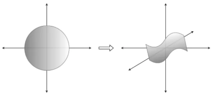
Figure 1. We effect random sampling in our model by passing a vector of
noise (random numbers) z to our model (equation 1). This transformation from a noise variable to a valid image of a tectonic plate arrangement can be thought of as a mapping from some full hypersphere (with
dimensionality equivalent to that of z) to a manifold space of lower dimension, which represents the space of valid output images.
the consistency of plate boundary reconstructions can be evaluated and gaps in observations can be filled. Thus, the problem can be addressed in a data-driven fashion; instead of attempting to fill-in regions where no seafloor data exist, for instance, by directly simulating underlying pro-cesses, we suppose that there is a distribution pdataof valid plate boundary images, that is, a manifold in the hyperspace of all possible plate bound-ary layout images from which we can sample and which can be learned from the geodynamic model. In other terms, the data distribution pdata is provided through a set Y = {yi}, i = 1 … N of images produced by a geodynamic modelP, the mantle convection model. This model will be described in more detail in section 3.
2.1. Generative Neural Models
We attempt to achieve inpainting by learning a statistical model of the self-organization of plate boundaries in the form of a continuous, differ-entiable, and parameterized function, called the generator model (this is not the mantle convection code), from which we can sample arbitrary images (divergence maps) by passing a noise vector z, that is,
̂𝑦 = (z, 𝜃G), (1)
where ̂𝑦 is a member of the modeled distribution pmodeland𝜃Gis the set over which is parameterized (classically called model parameters in machine learning). The training process aims to modify𝜃Gsuch that pmodelresembles pdata, and by extension, generated sampleŝ𝑦 resemble real data y as closely as possible. This relation can also be understood as mapping a hypersphere of dimension dim(z) of arbitrary noise vectors to a lower-dimensional manifold of possible tectonic plate arrangements, as in Figure 1.
The mapping and thus the model parameters 𝜃Gare learned from the data Y = {yi}. It is therefore impor-tant to point out, once more, that there are two models in our method: (i) a numerical and physical modelP capable of simulating instances of plate boundaries satisfying the desired properties of self-organization giv-ing horizontal divergence images yiand (ii) a statistical model trained on the data produced by P. As far as the convection model is concerned, a variety of numerical solutions with diverse combinations of mate-rial properties can be considered. In this work, we use only one single combination due to computational limitations.
In contrast toP, should be capable of producing predictions on missing data given provided sparse data. For this reason, we wish that the output of be conditioned on the surrounding input information. We there-fore modify so that it takes some conditioning data; in our application this is the discrete plate boundary image, denoted as x, which contains a missing region whose content we would like to estimate to produce the predicted complete image ̂𝑦:
̂𝑦 = (z, x, 𝜃G). (2)
In our application, a generator with tuned parameters 𝜃Gtransforms any input incomplete map of plate boundaries (x) into a complete one (̂𝑦), which respects the statistics of plate boundary distribution in a data set produced by geodynamic modeling. The inclusion of the noise vector z is a reflection of the fact that there may be many valid completions of the input image, and therefore, we wish to perform some sampling from this distribution of valid completions conditioned on the input image. In practice, we do not directly inject noise via the input; rather, we employ dropout to introduce stochasticity as in Isola et al. (2017). Dropout refers to the process of randomly disabling parameters in the network at training time and has been shown to help models generalize (Srivastava et al., 2014). Dropout is usually disabled outside of training time, but in this case its inclusion provides a source of random noise. Although the noise element is not strictly a vector input to the generator function, we retain z as an input in our notation to make explicit the presence of a noise component in the model.
Learning the parameters𝜃Gof such a generator model from data is a problem, which is addressed with a variety of techniques in machine learning. We adopted Generative Adversarial Networks (GANs; Goodfellow et al., 2014), in particular, the conditional variant CGAN (Mirza & Osindero, 2014). These methods realize the generator function as a deep neural network, a trainable nonlinear function decomposed into linear parts and element-wise nonlinearities. Classical supervised training (i.e., where the generator learns to produce
a single output designated as the ground truth) is not desirable, since for a single incomplete input plate configuration x, multiple complete output configurations ̂𝑦 might be possible. Instead of providing unique “correct” answers during training, we instead provide a binary validation of the “correctness” of the solution. In particular, the generator function is trained together with a second neural network called a Discriminator, which takes as input either the output of the generator or an image from the training data set Y and produces a binary prediction:
̂b = (𝑦, 𝜃D). (3)
The training procedure alternates between these two networks. The role of the discriminator is to estimate whether the input is from the data set (=real) or generated (=fake). The training algorithm solves a joint optimization procedure, which trains the discriminator to detect fake data and the generator to fool the dis-criminator. When trained to convergence, the generator outputs images, which the discriminator cannot distinguish from training data, which brings the distribution pmodelof the generator output close to the data distribution pdata. When training models in machine learning, we must define a function that expresses the “loss,” or difference between the intended and actual output. The aim of training is to adjust the parame-ters (in our case𝜃G,𝜃D) to minimize the loss. The term “loss” in machine learning stands for misfit. The optimized loss function for the generator-discriminator pair is given as
adv=E𝑦[log(𝑦, 𝜃D)] +E(x,z)[log(1 −((z, x, 𝜃G), 𝜃D))], (4) which needs to be minimized with respect to the generator parameters and maximized with respect to the discriminator parameters, giving
min 𝜃G
max 𝜃D
E𝑦[log(𝑦, 𝜃D)] +E(x,z)[log(1 −((z, x, 𝜃G), 𝜃D))], (5) which is a two-player min-max game. The minimization and maximization over the networks and are carried out over their respective parameters𝜃Gand𝜃D. TheE operator is the expectation, which in the loss function can be understood as an average across the elements denoted by the subindex of the operator. For example, in the right-hand terms of equations (4) and (5), the expectation amounts to the average of the term inside the square brackets across all input incomplete images x and all possible values of the noise variable z. The loss function shown in equation (4) is commonly referred to as the adversarial loss, as the term captures the behavior of two separate models acting in opposition, or adversarially to one another. These generative models have been widely used in computer vision and computer graphics to produce nat-ural images of animals and clothing items (Isola et al., 2017) but also to sample output of physical processes like terrain (Guerin et al., 2017).
2.2. Learning Self-Organization
We are interested in predicting discrete data, in particular positions of ridges, subduction zones, and plate interiors, from discrete input of the same type, where parts of the data are missing. Performing these pre-dictions on previously unseen plate configurations is a hard problem, which requires the model to pick up underlying regularities, that is, the self-organization of plate boundaries. The goal is to capture the regu-larities described by the equations of the mantle convection modelP. The success of this strategy depends on various parameters: the capacity of the statistical model (in terms of mathematical expressivity), the amount of available training data, and the performance of the training algorithm.
In this work we propose to benefit from the rich output of the mantle convection codeP, which is capable of not only producing the desired discrete quantities (positions of ridges, subduction zones, and plate) but also intermediate numerical observations, such as local horizontal divergence. We argue that these intermediate variables contain more information than the discrete output and that they are thus better suited for learning the regularities of the underlying physical process. However, the downside to this potential strategy is that these quantities are only available for simulated data and in the final application the input will be a discrete plate boundary map provided by a domain expert. A model trained on this intermediate, continuous input data will be unable to perform predictions directly on discrete input data, as the input image modality during training time and in the final application must be identical.
As a consequence, the input to our generator during training is required to be a discrete image, thus allowing predictions from discrete input in the end application. However, we here benefit from a simple mathematical relationship between the continuous divergence field and the discrete feature positions: Low
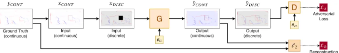
Figure 2. The generative model, which combines the rich entropy (in the sense of information theory) in divergence
fields as targeted output during training with the possibility of using discrete input and output (positions of ridges, subduction zones, and plates) during testing.
absolute values of divergence (close to zero) correspond to plates, high values of divergence to ridges, and low values to subduction zones. Discrete images can therefore be produced from continuous divergence fields by simple thresholding techniques. This suggests the following strategy: The generator takes discrete images as input and produces continuous divergence fields as output. This output is then thresholded to produce the desired discrete predictions. Similarly, the discrete input to is based on thresholded continuous input. This strategy combines two advantages:
• The learned model is capable of producing discrete output from discrete input with missing data, as desired.
• Requiring the model to predict divergence fields instead of the discrete output directly favors learning of the properties of the underlying physical process instead of simple geometric regularities, like connecting lines and extending curves.
This leads to the following categories of data: continuous ground truth yCONTand continuous predictions ̂𝑦CONT, continuous input xCONTproduced by masking out a region of yCONT, discrete input xDISCproduced by thresholding xCONT, and discrete output ̂𝑦DISC produced by thresholding ̂𝑦CONT. This can be pictured schematically as in Figure 2.
As is classically done when training GANs, we complement the adversarial loss given in equation (4) with a supervised loss, which directly minimizes the per-pixel𝓁2reconstruction error of the continuous output:
R=|| ̂𝑦 − 𝑦||2, (6)
where ̂𝑦 is the predicted continuous output and y is the continuous ground truth image from the training set. Both are complete data images, without any missing region. This loss is combined with the adversarial loss (equation (4)) giving rise to the full loss function:
= adv+R. (7)
The roles of these two losses are different. The adversarial loss is responsible for learning the manifold of physically plausible images. In theory, it should be sufficient and optimal. In practice, manifold learning from limited amounts of training data is difficult, as the binary loss signal is too weak to learn. This makes it necessary to water down the training objective by providing a loss directly related to the reconstruction of missing data, as is now generally done in the GAN literature. This supervised loss has the drawback of assuming a single solution for the prediction of the missing data, whereas manifold learning considers a set of possible solutions. On the other hand, it provides a richer training signal and stabilizes training.
2.3. Experimental Protocol
The training data set is composed of divergence images computed by the convection modelP. From a single divergence field, we produce input/output pairs (xDISC, yCONT)by first randomly masking a region to simulate the absence of observations and then thresholding and skeletonizing (an image analysis technique that reduces shapes into line segments) the continuous image to extract discrete ridges and trenches. The masked image defines the input xDISC, whereas the original continuous image also serves the target output yCONT. This allows the model to be trained with full supervision (i.e., the desired output is fully known). Figure 3 shows an example plate boundary image generated from a divergence image.
As is common practice in machine learning, the data set of available images is divided such that one subset is used for training, that is, minimizing equation (7); one subset is used for validation, that is, choosing
Figure 3. An example divergence image, the value of the divergence being normalized by the maximum value (left), and the resulting plate boundary image
(right) once thresholding and skeletonisation have been applied. Red pixels in the later image represent ridges, blue pixels indicate subduction zones, and light-gray pixels are plate class.
hyperparameters of the model such as architecture or learning rate; the final subset is used for evaluation. We use 1,000 training images, 300 validation images, and 300 test images.
We implement the statistical neural model as a deep neural network. We incorporate design elements such that
1. incomplete input images are condensed into vector representations, which encode the overall regularities of the layout, from which the complete output image is decoded;
2. the neural model considers regions of interest across the whole image, instead of just a small local area, a mechanism called “self-attention”; and
3. a trivial solution of inpainting only plate class pixels will be penalized through balancing and weighting. The details of these elements are given in the appendix.
3. The Physical Model
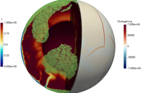
We build a database of images of the horizontal divergence field at the surface of a convection modelP dis-playing plate-like behavior. Unfortunately, this model is a convection model with intrinsic numerical and physical simplifications, and hence, we face strong limitations to use it for real cases with geological data. Therefore, we choose a model with which we have the capacity to generate a large number of images that are not too correlated. The case we define as a target experiment corresponds to the model presented in Mallard et al. (2016) with intermediate yield stress, adding up stiff continental rafts (see Figure 4). The vigor of convection is about 10 times smaller than that of the Earth (the surface velocity is close to 1 cm/year). A total
Figure 4. Three-dimensional snapshot of the nondimensional temperature field inside the shell, nondimensional
of 95% of the heat budget comes from volumetric heating rate, the remaining 5% coming from the base. For simplicity, we neglected chemical heterogeneity in the deep mantle. These models rarely display pure trans-form shear zones (i.e., where the horizontal divergence is zero), contrarily to more sophisticated models (Coltice et al., 2017). Therefore, the divergence field gives hereafter a comprehensive view of the location of plate boundaries. To simplify the problem even more, we fix the positions of continents over the run, corre-sponding to the present-day configuration, such that a test against the plate layout of the Earth today can be performed, in order to evaluate how far we are from applying our technique to observations. The fixity of con-tinents is clearly not realistic, but the goal here is to realize an anticipation exercise that remains tractable. We hence avoid modeling continent motion by advocating tracers, which is computationally expensive. We solve the equations of conservation of mass, momentum, and energy considering incompressible mantle under the Boussinesq approximation using the StagYY code (Tackley, 2008). Nondimensional viscosity𝜂 follows the modified Arrhenius law and is strongly temperature and pressure dependent:
𝜂(z, T) = 𝜂0(z)exp ( E a T +1− Ea 2 ) , (8)
where Eais the nondimensional activation energy equal to 30, leading to maximum viscosity contrasts of 6 order of magnitude over the model, and T the nondimensional temperature. We add a viscosity jump by a factor of 30 at 660 km depth, the limit between the upper and lower mantle, as suggested by postglacial rebound (Mitrovica & Forte, 1997) and geoid studies (Hager, 1984; Ricard et al., 1993). The viscosity of 290 km thick continental rafts is 100 times higher than the mantle.
To localize deformation in narrow regions (which are typically ∼300 km broad in this model), we use a pseudoplastic rheology (Moresi & Solomatov, 1998; Tackley, 2000). When reaching a yield stress𝜎Y, mantle
material undergoes instantaneous pseudo-plastic weakening, which is simulated by a drop of the viscosity as a function of the strain rate:
𝜂Y=
𝜎Y
2𝜖.II , (9)
where𝜖.IIis the second invariant of the strain rate tensor. The nondimensional value of the yield stress is
here 1.5104, and continents cannot yield. We refer to Mallard et al. (2016) and Rolf and Tackley (2011) for
more detailed information on the modeling.
We perform a calculation at statistically steady state corresponding to about 480 transit times (one transit time being the time a slab would reach the base of the mantle if sinking at the rms surface velocity) that would scale to approximately 36 Gy for the Earth, to generate 1,800 different snapshots of the horizontal divergence field at the surface (one every 20 million years), that highlights the location of convergent sub-duction zones at divergent ridges. Among all the simplifications, we make to put all our efforts into the machine learning scheme; the images we make are flat and do not take sphericity into account.
There is some degree of correlation between subsequent images, as a visual inspection shows some evidence of structural similarity between consecutive examples. When splitting the images into training, validation, and test subsets, we therefore place gaps of 100 unused images between these subsets. Ideally, we would pick one snapshot every 300 My (Bocher et al., 2016) and produce 10 times more images. Unfortunately, computing such a data set already takes 45 days on a supercomputer.
4. Experimental Results
The neural model was implemented in the Python language and using the PyTorch framework (Paszke et al., 2017), with initial code structure based on the pix2pix/CycleGAN code (Isola et al., 2017). The parameters were trained on the training set (see section 2.3) with the Adam optimizer (Kingma & Ba, 2014), and the two-time scale update rule (Heusel et al., 2017) with a learning rate of 0.0001 for the generator and 0.0004 for the discriminator. The neural architecture (numbers of layers, filters, etc.) was optimized on the validation set. We in particular refer to the appendix for detailed description of
• the function forms of the neural networks (their architectures), • the way we control attention to parts of the input (“self-attention”), and • the way we control sparsity through weighting.
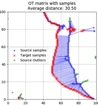
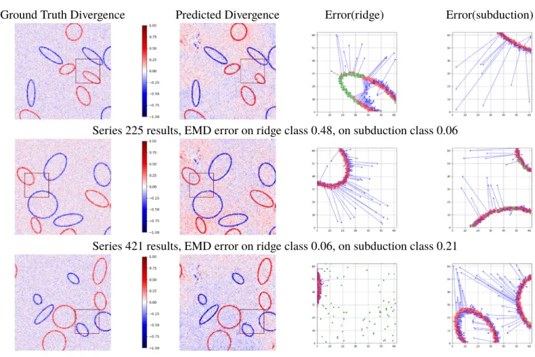
Figure 5. An illustrative example of the optimal pairing of ground truth
pixels and predicted structures, as well as the mean distance between them.
We provide performance numbers on the test set, which was not used for any training or hyper-parameter optimization.
4.1. Evaluation Metrics for Sparse Images
Evaluating generative models is difficult by nature, as objective metrics are difficult to find. Measuring reconstruction loss is suboptimal, since the stochastic nature of the problem allows for multiple possible predic-tions for a given input—let us recall that our goal is to learn the manifold of all possible solutions.
The literature on generative neural models (GANs, Goodfellow et al., 2014; Variational Auto Encoders, Kingma & Welling, 2014; and Autore-gressive Generative Models, van den Oord et al., 2016) was based for a long time on qualitative evaluation, which is possible when the image domain is natural images like faces, animals, or landscapes. The need for quantitative evaluation was soon evident, and evaluation metrics were proposed. The most widely used ones are Inception Score and Fréchet Inception Distance, based upon the idea that a classification network trained on the standard ImageNet data set can stand in for a human observer to assess generated image quality (Heusel et al., 2017; Salimans et al., 2016). This idea is far from perfect, as a discriminative score (clas-sification score) is used to assess image quality. More importantly, these two metrics cannot be applied to our work, since our images are not natu-ral ones. A modification of the score to our setting is not straightforward, as no direct taxonomy of the plate images (required for classification) is possible.
For this reason, we propose to fall back to evaluating the model by measuring reconstruction loss on the image simulated by the physical modelP, taken from the test set. Using any pixel-wise loss, as for instance 𝓁1or𝓁2normed difference, would be nonsuitable, as the content of our images is highly structured and the
support of ridges and subduction zones is very small. Structures that have been correctly predicted but at a location shifted from the ground truth location would result in zero overlap and therefore maximum error, which is not desired.
We therefore instead use Wasserstein or Earth mover's distance (EMD; Villani, 2008) as a metric: W (Pa, Pb) =𝛾∈Π(infP
a,Pb)
E(t,u)∼𝛾[||t − u|| ] , (10) where𝛾 is a transport plan, that is, what proportion of mass to move from point t in the distribution Pato point u in the distributionPb.E is the again the expectation, which can be understood as a weighted average over all distances||t − u|| and thus gives a sense of the overall “work” required to transform one distribution to another under a transport plan𝛾. This metric can be intuitively understood as the expected work (in terms of horizontal Euclidean distance) to optimally transport a pile of Earth from one location to another, hence the name “Earth mover's distance.” In practice our units are indivisible discrete pixels, and we can treat this as an optimal matching problem. We can thus determine the optimal transport solution between predicted and ground truth images using, for example, the Hungarian method (Kuhn, 1955). The final EMD metric is taken as the mean Euclidean distance between paired predicted and ground truth pixels, with a penalty distance applied to any unmatched point.
Figure 5 shows an example output of pixels paired with the Hungarian method. The ground truth pixels are marked in red, and the predicted pixels in blue, and optimally paired points joined by a blue line. Outliers (false positives or negatives) are indicated in green, and each is assigned the diagonal size in pixels of the inspected region as a penalty distance.
As the neural model outputs a continuous image, we must first convert to a discrete, three-channel image (one for ridges, one for trenches, and one for plates' interiors). This requires a choice of threshold level, and we have envisaged that the end-user would manually select this threshold themselves to produce the best result. In the absence of a user to choose the threshold during evaluation, we instead perform an automated search for the threshold, which will maximize the EMD evaluation metric. This perhaps qualifies as
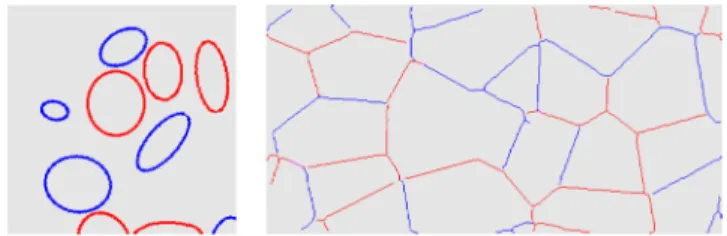
Figure 6. Example of a synthetic image created with simpler and geometric
only self-organization: circles (left) and Voronoi regions calculated from random point clouds (right).
optimizing over the metric, which was noted by Barratt and Sharma (2018) to possibly produce adversarial examples; however, we did not find this to be an issue in our experiments.
4.2. Validation on Simple Shapes
In contrast to the evaluation of natural images like faces and people, qual-itatively evaluating the produced output of geodynamical data is difficult, even for a human expert. We therefore evaluate the model first on data with simple geometrical regularities, which requires simpler reasoning like connecting lines and extending arcs. In this data we do not find any properties specific to mantle convection, but we use similar structures to the geodynamic model, with curved linear shapes.
We propose two different data sets of simple geometrical shapes:
Circles and Ellipses —we created a set of constant plate images on which we superposed a number of
random circles and ellipses of random classes ridge and subduction.
The continuous “divergence” image in this case was created by assigning a scalar value from a Gaus-sian distribution for each pixel, which was parameterized based on the class membership of the pixel in question, that is,
𝑦DIV(i) = (𝜇k, 𝜎k), (11)
where, as in (A1), k ∈ [0, 1, 2] is the class of the pixel at location i in the image yDISC, represent-ing ridge, plate, or subduction zone. The discrete input image is then created by thresholdrepresent-ing and masked to remove a region as with the geodynamic data. Note that while the problem is similar in that we try to have a neural model learn a mapping from a discrete value to a range of possible continuous value, this is not true physical divergence at all. We use the term “divergence” in this manuscript only for the purpose of analogy.
Voronoi plates —we created synthetic plate boundary images by first taking a sample of random points
upon the image, calculating the Voronoi diagram of this point cloud, then defining the resulting Voronoi regions as plates. Random velocity directions are then assigned to each plate, from which a divergence field can be calculated.
An example of each class of image is shown in Figure 6. The EMD metric results for the circles, ellipses, and Voronoi data are shown in Table 1. Note that the EMD is normalized by the diagonal mask size.
Some example result images for the ellipses- and Voronoi-based data sets are shown in Figures 7 and 8, respectively. The reconstruction loss is confined to the local region within the mask, while the adversarial loss was applied to the entire image. Therefore, we are not concerned with any errors or artifacts outside of the mask region, as we can always cut and paste the inpainted region into the original input image. Outliers (shown in green) show points that the model has failed to inpaint, or where it has erroneously painted pixels.
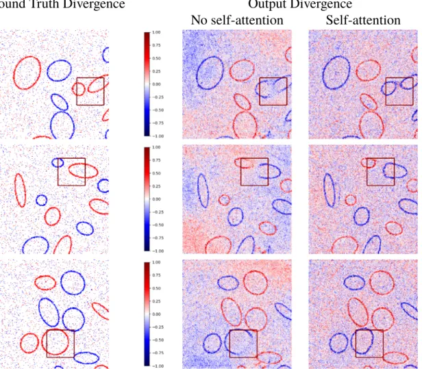
Of particular interest in these results is the effect that the self-attention has on the completions of the ellipses, a procedure that we detail fully in the appendix. In essence, self-attention allows the neural network to link the output (prediction) of a value of a certain location to any possible input position, even far away without the need of a full traversal of the network—mathematical details are given in the appendix. Some examples
Table 1
Prediction Results on Simple Geometrical Data (Circles, Ellipses, and Voronoi plates) Measured With Normalized Earth Mover's Distance
Data set Norm. EMD
Nonfilled circles 0.31
Ellipses 0.23
Voronoi 0.24
of the effect are shown in Figure 9. Without self-attention layers the ellipse outlines are left incomplete with ragged ends. If self-attention is included, the ellipses (while occasionally slightly misshapen) are given fully closed outlines.
4.3. Geodynamic Tests
Using the synthetic geodynamic data produced by the physical modelP described in section 3, we tested the model's ability to inpaint a missing region, that is, to place missing plate boundaries of the right type at the right location. We also tested the discriminator's ability to distinguish real and fake plate layout images after training and the effect of changing mask size on the inpainting error.
Figure 7. Results from the ellipse data set with both𝓁2and adversarial loss applied to output divergence image. The input is the ground truth, with the area
inside the marked square removed.
4.3.1. Completion
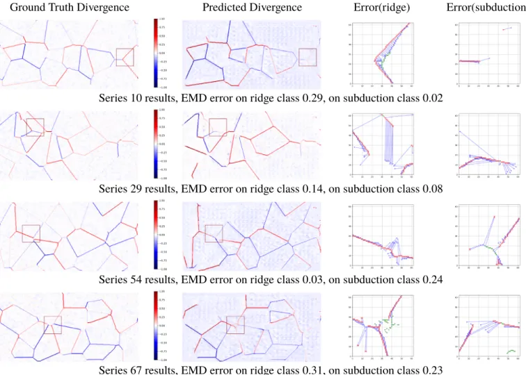
As shown in Figure 10, the quality of predictions is diverse. The prediction for Example 1 is nearly perfect, prolongating the trench and back-arc ridge. Example 2 predictions are correct for the trench along the con-tinent, the trench on the north side, and proposes the existence of a divergent region. But in some cases the trench is not well predicted, and some convergent regions are in the ocean where they should not appear. Example 3 shows a correct prolongation of a ridge system, while Example 4 is a case where prediction is wrong. Overall the model correctly sets ridges and subduction boundaries with cases where a stroke passes completely through the masked region (Example 1) and does reasonably well in cases where a line begins outside the mask and terminates within the masked region (Example 3). Where the model fails are the instances where there is some structure completely contained within the mask region as in Example 2—the ridge strokes have been completely removed in the input to the model, and they are not replaced. Example 4 is similar.
Figure 11 shows an example of the variation seen in the output when the model is repeatedly run, with the random seed for the dropout process changing each time. There is noticeable variation in the outputs, but it is not extreme; the completions adhere to the same overall structure.
4.3.2. Effect of Mask Area
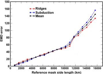
We test the effect of mask size on the accuracy of inpainting. We expect that as the mask area increases, so will the error. As explained above, our maps are considered as rectangles, not unfolded spheres. Therefore, mask size corresponds here to a case where all latitude circles have the same length as longitude great circles. Figure 12 shows the effect of changing mask size on the EMD error. This plot shows the results obtained by testing different mask sizes on a model trained with a reference mask side length of 6,000 km. It is hardly surprising that the error increases with mask size. The slope of the graph is steady until approximately
Figure 8. Results from the “Voronoi plate” data set with both𝓁2and adversarial loss applied to output divergence image. The input to the model is created by
masking a region out of the ground truth, as in Figure 7.
11,000 km side length, which in terms of the image would obscure approximately half the image. The slope then increases at a greater rate. As mentioned, this is tested on a model trained with only one mask size. Without further experiments we cannot firmly deduce whether this error increase is due to the model being untrained to deal with large mask sizes, whether there is insufficient structure to infer the masked region contents or both.
4.3.3. Discriminator Detecting Real/Fake Images
We test the ability of the discriminator network to recognize valid versus invalid plate layout images. The motivation is that even if a completed image is created by some means other than the generator, it could potentially be given to a pretrained discriminator to verify whether the suggested image completion is valid. To perform this test, we input ellipse, circle, and Voronoi data to a discriminator trained on synthetic geody-namic data. We also pass a new set of synthetic geodygeody-namic data, which was built from former 3-D spherical calculation of convection, with different parameters: We used the model of Mallard et al. (2016) without continents, and the models used in Sim et al. (2016) with different continent sizes, and the model presented in Coltice et al. (2017) with a more realistic rheology.
As the discriminator outputs a scalar value that scores the “realness” of the input (higher means more likely to be real and lower means less likely), we expect the output to be highest for the synthetic geodynamic data input, then progressively lower for the Voronoi, ellipse, and circle data in that order as they become obviously more likely to be invalid.
Figure 13 shows the results of this test. After 1,000 iterations through the full data set (an intermediate stage of training) we see a clear division of the discriminator output between training data sets, decreasing in the
Figure 9. Results from ellipse data set, with and without self-attention, a mechanism short-cutting spatial long-run dependencies between input and output
locations (see Appendix A1). Without self-attention, the model can fail to draw complete ellipses, while with self-attention the ellipses are closed shapes, even if they are somewhat misshapen.
expected order. However, at the end of training, the discriminator has begun to confuse Voronoi and geo-dynamic data and is less confident in telling real and fake data apart. This is perhaps unsurprising, as by the end of training, the discriminator is being passed real and fake images, which look very similar (i.e., at this point the generator is capable of producing very convincing images) and being told that they are somehow different, and it is somewhat unclear upon exactly what criteria it is learning to accept and reject samples. We had assumed that over the course of training, the discriminator would simply fine-tune its abil-ity to identify fake samples based on increasingly subtle detail. Some GAN implementations, for example, that of pix2pix (Isola et al., 2017) include the option of passing the discriminator an image pool of cached images, which have been randomly sampled across training. This is a means of forcing the discriminator to “remember” what it previously considered fake. Such an approach may be necessary here to produce a use-ful discriminator by the end of training. By “useuse-ful” we here mean useuse-ful for distinguishing different data sets. Fine-tuning does not prevent the discriminator from providing useful information to the generator for learning the manifold of valid images.
Another possibility is to force the model to fine-tune by reducing the learning rate. This will prevent the learning scheme from making any sudden changes, which we observe in Figure 13 around epoch 1,000. Running this discriminator test during the course of training will give an indication of when it is appropriate to restart training with a reduced learning rate.
Figure 10. Results from synthetic geological data set with both𝓁2and adversarial loss applied to output divergence image. Values are normalized, and
continent locations are shown in green. Note that although there are some differences outside the missing region, we do not overly concern ourselves with these, as the nonmissing regions can simply be copy-pasted into the final output image if necessary. As yet we have no explanation as to why we sometimes observe differences in the nonmissing regions.
4.4. Earth
Figure 14 shows some example results for a synthetic data-trained scheme tested with the present-day plate boundary network on Earth as input data. It is immediately obvious from visual inspection that the results are not as good as those obtained on a synthetic-trained and synthetic-tested model. Even in cases where the EMD error obtained is comparable, that is, for the subduction class in the first example and the ridge class in the second, the inpainting is poor and in fact fails where we typically see the model succeed—a smooth continuation of a stroke traversing the mask. It is easier to observe in the discrete images from the real Earth data set, but these inputs are somewhat busier than the inputs the model was trained on. The physical parameters used to produce the training data are not identical to Earth's, and this clearly has an
Figure 11. Examples of how the output varies with changes in the noise
component z. The full ground truth image is shown on the left. The image on the right shows nine different suggested completions in each of the outer cells, the center being a copy of the ground truth mask region. Note that because we use dropout to introduce stochasticity, we cannot directly measure to what extent the output varies with changes in the noise component. Qualitatively, the differences are noticeable, but not extreme, with the completions occupying the same approximate position across each of the examples.
impact on the model's ability to successfully inpaint. It may thus be nec-essary to train the model on a suite of data seeded from varying physical parameters and impose some degree of supervision, aiding the model to distinguish and perhaps adapt to variations in physical parameters. It is also interesting to note the roughly Australia-shaped completion in the second example, where it is not present in the ground truth. This may indicate some overfitting, which will not be picked up when testing the synthetically trained model, as the Australia boundary is a common feature in many examples in the training and test data sets. This then suggests that there is not sufficient independence between the test and training data sets to appropriately test the model's ability to generalize.
4.5. Ablation Study
We undertake a sensitivity study, called ablation study in machine learn-ing, removing selected components from our model, to investigate the impact each piece of the architecture has on the performance of the machine learning model. The results of the ablation study are shown in Table 2, where each column indicates an element's inclusion. A model without intermediate variable out-put produces a discrete image directly, rather than producing a divergence image. The weighting column refers to a per-pixel weighting applied to the reconstruction loss term, which better copes with imbalanced data—see Appendix A2 for details. The base model is shown on the bottom row and has all modifications included. Note that an EMD metric of 1.0 indicates that the overall the output is completely dominated by false positives or false negatives (more often it is the latter).
Removing the intermediate variables has a large effect on the EMD, often resulting in the model failing to inpaint anything at all. Removing the reconstruction loss weighting (see Appendix A2) causes a slight improvement in the EMD, while removing the self-attention layers (see Appendix A1) from the discrimina-tor cause it to deteriorate. Removing both features results in a slightly better EMD than the baseline (similar to no weighting) but achieves this result after another 1,000 epochs of training time (approximately 1 day in wall-clock time on our computation cluster), and a worse local𝓁2loss. We note also that the exclusion of
either or both the self-attention layers and reconstruction loss results in artifacts in the output divergence image, and this is reflected in the local𝓁2loss in Table 2, which (while not a perfect metric) shows a
cor-responding increase in error when self-attention is removed. This is not a large concern, however, as these artifacts tend to be removed by the thresholding and skeletonization operators. However, while the end
Figure 12. Effect of changing mask area on error, normalized by mask size.
The reference mask side length refers to the size of the masked area at the equator. The mask size is kept consistent as it is moved across the projected image, thus its effective size changes depending on location.
product is unaffected, this perhaps reflects a deficiency in the extent to which the model has learned the intermediate representation.
5. Discussion
We proposed an anticipation experiment for plate tectonics in the digital age: Geodynamic models will be able to capture the essential self-organization of plate boundary geometry, and artificial intelligence frameworks can learn from them to help scientists to position plate boundaries in areas where observations are lacking. But this is futuristic, and the present experiment shows where we stand. The current state of the art in machine learning requires a large amount of data in order to learn complex regularities, in our case the self-organization of plates; we think that a larger amount of data (an order of magnitude more at least) is necessary to answer this question.
One of the key design features of our proposed method was to cast the problem as the prediction of continuous intermediate variables (the diver-gence field) from discrete input. Results have confirmed the intuition that these variables are more closely related to the regularities we aim to capture.
Figure 13. Discriminator output for different data sets across all epochs,
where a single epoch is one pass over the full training data set.
In the framework we have designed, attention schemes are an impor-tant inclusion, given the sparsity of the image data. Emphasizing the plate boundaries on the basis of their pixel area is an obvious first step, but it is possible that there are regularities in the surrounding plate area and shape that we are effectively telling the model to ignore with this scheme. The learnable self-attention scheme (see Appendix A1) presents an opportunity to overcome this limitation and learn the most effective weighting scheme. The effect on EMD is noticeable, but self-attention also reflects the notion of interdependency between every location in the self-organization of the tectonic plates.
Evaluation is an ill-posed problem in this application, as it is many to one. That is, for a given input, there are many possible completions, whereas we only have a single paired ground truth image, which presents just one possible solution. We would like to propose a manifold of solutions, from which the scientist would choose in the end, not the machine. The EMD metric does a good job of expressing the structural difference between the predicted and ground truth images but cannot compare against a ground truth it does not have; therefore, it cannot give us an indication of the overall feasibility of an image, irre-spective of whether or not it matches the ground truth. For this reason, it is necessary to have a metric that analyzes the underlying features or structure of an output in order to evaluate it, which is essentially what common metrics in GAN literature do. However, these are trained on data sets containing millions of images, which our specialized data set cannot compete with. Another way to evaluate the proposed solution is to perform the kinematic reconstruction and confront it to independent observations.
The broader question is how well the model generalizes. Inpainting results are satisfactory, yet we note that visually, there is some similarity between samples. We wish the model to learn the rules that govern a plate layout, as opposed to memorizing a suite of images and inserting the necessary patch. The best method we have to test this is with a hold-out set of unseen test data, but if the similarities between the training
Figure 14. Results from testing with real Earth geological data on a model trained on synthetic data. Values are normalized, and continent locations are shown
in green. The completions are not satisfactory, even if the reported EMD error is low, the strokes are broken rather than smooth. Note also that the predicted divergence has some biasing, in that the plate region is colored slightly red or blue. In practice, this bias is eliminated when creating the output discrete image.
Table 2
Ablation Study Results
Self attention Weighting
Intermediate variables (Appendix A1) (Appendix A2) Local𝓁2(×10−3) EMD
− − − N/A 1.0 × × − 5.18 0.22 × − × 5.51 0.25 × − − 8.16 0.22 − × × N/A 1.0 × × × 4.89 0.23
Note.“×” indicates the presence of a feature; “−” indicates its absence.
and test data are too great, this method begins to break down. With a sufficiently large and diverse data set, this is less of a concern. Improving the data set requires that more appropriate models with moving continents, higher convective vigor, free surface, chemical heterogeneity, damage, and healing should be run and stored. Unfortunately, this must be relegated to the future because some of these issues are not fully understood yet in terms of physics; they are not implemented in 3-D spherical convection models, or they are too computationally expensive. Will we be able to build such data set within the next decade?
In the absence of a larger geodynamic data set, we can design and test models on synthetic data sets, which encapsulate simplified aspects of the problem we wish to solve. Simplifying the problem this way and cre-ating large quantities of synthetic data allows us to test what is a model limitation and what is a data limitation. In the example of the ellipse and Voronoi data above, we have simplified the nature of the com-pletions, which makes visual verification trivial but also confirms that the proposed model can recognize and complete at least very simple structures. Conceptually, there is still some distance between these syn-thetic data sets and the geodynamic data. For example, the Voronoi-based data are more connected and feature many cases of strokes passing straight through the mask region, which the model tends to have no difficulty inpainting. Further, the fake plate distribution in these images is created by randomly placing points, then randomly assigning velocities to the resultant Voronoi regions. There is no underlying regu-larity for the model to learn, only randomness. The size distribution of the Voronoi regions also does not match that of the Earth. This could be rectified at the time of data set generation, by creating the plates with a split-and-merge approach until the desired distribution shape is reached. However, the plate area distribution may have evolved on our planet (Morra et al., 2013), which makes the task more complicated. To finish with the limitations of the framework, we acknowledge that the Earth is not flat and that the images have to be treated on a sphere. This is not a trivial task for the machine learning scheme, but some methods of applying common deep learning techniques to spherical surfaces are under development (Cohen et al., 2018).
Future work will address the possibility of model-based Deep Learning, that is, the creation of neural models with specific inductive biases, which model prior knowledge on the physical processes at hand. Similar approaches have been recently studied in physics (de Bézenac et al., 2017).
6. Conclusions
In this manuscript, we have designed and tested a framework to expand plate tectonics in a futuristic way, exploring how the digital age could provide new means for geoscientists to reconstruct the tectonic evo-lution of our planet. We have considered that 3-D spherical convection models producing self-consistently plate-like behavior is the first pillar: They can overcome some limitations of plate tectonics and use the physics as an additional source of information on the self-organization of plate boundaries. Although sig-nificant limitations of these models are acknowledged, their development is promising. The second pillar is the growth of artificial intelligence, which is an ideal tool to learn self-organization from these models. Geo-scientists can then use this knowledge to fill observational gaps and build physically sound plate layouts. The goal here is to give new tools for human decision, not to have the machine provide a unique solution. Inverse methods could work out such problem, but each new inpainting would be required to solve the
costly inverse problem, whereas using a trained neural network is almost instantaneous. The computational effort is expended only once, for training and testing.
Our GAN framework with self-attention takes as input the location of ridges and trenches and the posi-tion of the unknown region. The output is a divergence map from which ridge and trench geometries are extracted. We benchmark the procedure against simple data sets (circles, ellipses, and Voronoi plates) for which we have a large amount of images (>10,000). Our model produces satisfactory results on data gener-ated by geodynamic calculations, for interpolating or terminating a plate boundary. However, structures that are completely contained in the inpainting regions are not robustly reconstructed yet. The EMD works well as an evaluation metric when the ground truth is known, but independent geological data would have to be used when evaluating solutions proposed for the Earth. At least, benchmarking for completing plate boundaries in a region of the Earth today is necessary. In our case, the geodynamic model is too simple, and the amount of images in the data set too low to give appropriate solutions. Before geodynamic models and machine learning schemes are at the level to make this futuristic framework sensible, the only solu-tions to fill observational gaps with plate tectonics theory are to look for new data coming from rocks or indirectly with geophysics. But as our study shows, new solutions for problems where no observations exist are emerging.
Appendix A: Neural Architectures
The statistical neural model described in section 2 and composed of a generator and a discriminator has been implemented as a deep neural network with architectures specifically designed for this problem and optimized on the validation data set. Deep neural networks are in essence highly nonlinear functions, which are parameterized by a set of weights learned from data. The functional form of these networks is deter-mined by their architecture, that is, the way a large function decomposes into a set of smaller mathematical building blocks (functionals), which are combined through function composition, that is, f(x) = g(h(x)). This appendix details the architectures we chose for the specific problem of tectonic plate prediction. They are variants of architectures widely used in computer vision.
The generator function is implemented as a U-Net (Ronneberger et al., 2015), which features an encod-ing + downsamplencod-ing stage and a decodencod-ing + upsamplencod-ing stage, with additional skip connections between corresponding resolutions in the separate downsampling/upsampling stages. In simplified terms, U-Net starts by condensing (encoding + downsampling) the full information of the image into a minimal amount of relevant information (here we look for the simplest description of the distribution of ridges, trenches, and plate interiors). Then, the U-Net uses this reduced information to progressively generate (decod-ing + upsampl(decod-ing) a new image respect(decod-ing the organization extracted in the first stage. In terms of computational steps, the output of layer n is concatenated with the output of layer N − n − 1 and given as input to layer N − n, where N is the total number of layers in the network. These connections allow us to more directly incorporate details from the different resolutions of the input images into the same resolution output images. The generator neural model architecture, including these skip layers, is shown schematically in Figure A1.
To encode the input for the generator, we created a binary mask representation , which is 1 in the missing image region and 0 elsewhere. We define the input discrete image x (we temporarily drop theDISC subscript for cleaner notation) at pixel index i and channel j as
xi𝑗= {
𝛿𝑗k if i=0
0 if i=1 , (A1)
where𝛿 is the Kronecker delta
𝛿𝑗k= {
1 if i =𝑗
0 if i≠ 𝑗 (A2)
and k ∈ [0, 1, 2] is the class of the pixel at index i, either ridge, plate, or subduction, respectively. The input image xDISCis then a one-hot representation of the pixel classes, everywhere except for the missing region, which is set to zero.
The discriminator is implemented as a convolutional neural network. Convolutional neural networks analyze subportions of images and assemble the result of the analyzed portions into a reduced representa-tion, being a vector, or a code. From this representation of the original image, the discriminator determines
Figure A1. Diagram of the generator architecture, with downsampling and upsampling stages connected by skip layers as in U-Net architecture (Ronneberger
et al., 2015). Each box indicates a filtering operation, with the filter input-output dimensions given on the right. A black arrow shows where an image output by a filtering operation is passed as input to another filtering stage without scaling the image size up or down, while blue and red arrows indicate that the image is passed to a subsequent stage with downscaling or upscaling applied, respectively.
and returns a “real” or “fake” label. Through training, the parameters of each neuron, called weights, are optimized to obtain the best fit (minimum loss) to the answer. We use spectral normalization in the convolutional neural network architecture (Miyato et al., 2018) as an additional step during training where the singular values of each network layer's weight matrix are normalized such that the largest singular value is one. This places a constraint on the norm of the discriminator gradient pointing toward minimum loss, a condition that has been found to result in greater stability during GAN training (Gulrajani et al., 2017; Miyato et al., 2018; Odena et al., 2018, 2017). The input to is the output of concatenated channel-wise with .
A1. Self Attention in Neural Models
As mentioned, the neural model needs to capture the plate self-organization at several spatial scales, going from simple geometrical regularities to complex regularities arising from the mantle convection. It is the role of the discriminator to judge the validity of the generator's reasoning and to avoid validating inpainting of simple generated images. If, for instance, a masked region is inpainted with only plate pixels (and being mostly right, in terms of sheer pixel quantity), the resulting output would still have the overall “look” of a ground truth image.
In classical convolutional neural networks, regularities on a larger scale are handled through the deeper layers of the neural network, as a given convolutional layer takes into account only a local neighborhood (the neuron analyzes a region around a position). In particular, an output value q[i,𝑗l]at position (i, j) in a classical feature map q of layer l, that is, the output of a single layer is calculated as
q[i,𝑗l]= m−∑1
a=0
m−∑1
b=0