HAL Id: hal-01909701
https://hal.archives-ouvertes.fr/hal-01909701
Submitted on 31 Oct 2018HAL is a multi-disciplinary open access
archive for the deposit and dissemination of sci-entific research documents, whether they are pub-lished or not. The documents may come from
L’archive ouverte pluridisciplinaire HAL, est destinée au dépôt et à la diffusion de documents scientifiques de niveau recherche, publiés ou non, émanant des établissements d’enseignement et de
Fracture morphology and viscous transport
J. Schmittbuhl, A. Steyer, L. Jouniaux, Renaud Toussaint
To cite this version:
J. Schmittbuhl, A. Steyer, L. Jouniaux, Renaud Toussaint. Fracture morphology and viscous trans-port. International Journal of Rock Mechanics and Mining Sciences, Pergamon and Elsevier, 2008, 45 (3), pp.422 - 430. �10.1016/j.ijrmms.2007.07.007�. �hal-01909701�
Fracture morphology and viscous transport
J. Schmittbuhl, A. Steyer, L. Jouniaux and R. Toussaint
Institut de Physique du Globe de Strasbourg, UMR 7516, 5 rue Ren´e Descartes, 67084 Strasbourg Cedex, France
Abstract
The morphology of a fracture in a granite block is sampled using a high resolution profiler providing a 3999×4000 pixel image of the roughness. We checked that a self-affine model is an accurate geometrical model of the fracture morphology on the basis of a spectral analysis. We also estimated the topothesy of the experimental surface to be lr ≈ 2 10−7mm and the roughness exponent to be ζ ≈ 0.78. A finite
difference scheme of the Stokes equation was used to model the viscous flow through a fracture aperture that included the experimental fracture surface. It consists of a semi-fracture between a flat Plexiglas plate and the rough fracture surface. We finally compare our numerical results to experimental measurements of the fluid flux through the fracture using a glycerol/water mixture (to be at sufficiently low Reynolds number where Stokes equations holds). The comparison is successful de-spite a limited resolution of the experimental measurements. We finally show that only long wavelengths of the fracture control its hydraulic conductivity.
Key words: Fracture roughness, fluid flow, hydraulic conductivity
1 Introduction
The modelling of the fluid transport in low permeable crustal rocks is of cen-tral importance for many applications (Neuman, 2005). Among them is the monitoring of the geothermal circulations in the project of Soultz-sous-Forˆet, France (Bachler et al., 2003). The transit time of the brines into the natural and induced fractures between injection and production wells has to be care-fully estimated in order to provide precise estimates of the production running time. Water flux controls both the heat transfer to the fluid and the cooling of the massif (Murphy, 1979; Glover et al., 1998; Tournier et al., 2000).
As shown from previous studies (Benderitter and Elsass, 1995; Tournier et al., 2000; Evans et al., 2005) only a few important fractures, closely associated in clusters (Genter et al., 2000) are controlling the fluid exchange between
wells. Accordingly the study of the flow within a single fracture appears of central interest. It is also important for large scale numerical simulations of the convective circulation in the massif (Fontaine et al., 2001; Zhao et al., 2003). Up to now, only very simple models for fractures, i.e. parallel plates models, have been considered, ignoring the impact of the fracture morphology on the fracture transmissivity (Tournier et al., 2000).
For a parallel plate model, the steady state solution of the Navier-Stokes equa-tions for incompressible laminar flow yields the cubic law, where the volumetric flow rate Q depends linearly on the macroscopic pressure gradient in the flow direction, and is proportional to the cube of the plate separation a:
Q = −Ly
a3
12η∇P (1)
where Ly is the width of the fracture perpendicular to flow and η is the fluid
viscosity (Bodin et al., 2003; Brush and Thomson, 2003).
In this study, we are interested in the influence of a realistic geometry of the fracture on its hydraulic permeability (Brown, 1987; Plourabou et al., 1995; Hakami and Larsson, 1996; Adler and Thovert, 1999; M´eheust and Schmit-tbuhl, 2000, 2001, 2003). The morphology of fresh fractures is sampled and compared to a geometrical model that can be used in numerical codes for the fluid flow. We will also use the measured aperture profile as boundary condi-tions to simulacondi-tions. A contrario, the existence of a simple geometrical model of fracture morphology will allow to generate many realizations of synthetic fracture aperture, and thus study systematic effects when good statistics are needed. Our goal is to show that realistic fracture morphology can be intro-duced as a perturbation of the parallel plate model. However we show that strong influences on the transport properties might emerge owing to the long spatial correlations of the asperities morphology even in the limit of laminar flows. We have to mention that we assume that altered fractures partly coated with secondary minerals are still correctly described by a similar geometrical model (Schmittbuhl et al., 1993; M´eheust, 2002; Schmittbuhl et al., 2006). In any case, as long as the coating process redistribute masses within a finite range, the geometrical model considered will properly describe the large scale morphology of the fracture aperture – i.e., at first, only small scale modifica-tions of the aperture profile will happen. This large scale morphology will be shown to strongly control the fracture transmissivity, and the morphological model for fresh fracture is thus hopefully also relevant for the transmissivity of altered fractures.
We limit ourself to viscous flow characterized by low Reynolds number (Re 1) although turbulence might develop at high flow rate (Gutfraind and Hansen, 1995; Qian et al., 2005). The Reynolds number Re that can be defined from the
Navier-Stokes equation is the ratio of the inertial terms to the terms describing the viscous forces. Estimates of the velocity along the flow and estimates of velocity perpendicular to the main flow are respectively labelled uz and uh,
while lz and lh denote estimates of the respective scales of variation of the
velocities, and <a> the arithmetic mean aperture of the fracture. For viscous flow, uh is much smaller than uz, and lz much smaller than the mean aperture
<a>. Because of incompressibility, lz/lh ∼ uh/uz, which is vanishingly small,
and the Reynolds number can be evaluated as Re ≈ uzl2z/νlh, where ν = η/ρ
is the kinematic viscosity of the fluid (M´eheust, 2002).
We also assume that the lubrication approximation holds. Accordingly flow properties are only a function of the local apertures and not of the aperture gradients. This property implies that open fractures with different pairs of surface fractures, one on the top z+(x, y) and one on the bottom z−(x, y), but
with the same aperture field a(x, y) = z+(x, y) − z−(x, y), will have the same
hydraulic behavior. Among this set of equivalent fractures, a semi-fracture, made of a rough surface facing a flat plate can be defined as z+(x, y) = a(x, y)
and z−(x, y) = 0. This equivalent semi-fracture will show the same aperture
field. We will base our experimental approach on this property and reduce our problem to such a semi- rough fracture. The flat plate is chosen to be transparent (PMMA) which allow to follow optically tracers if necessary (e.g. in ongoing experiments on reactive fluids).
2 Fracture morphology
2.1 Roughness measurement
We studied the viscous flow imposed inside a fresh fracture that extends over an area of 10cm×10cm. Grains are typically millimetric (0.5mm). The frac-ture was obtained from a mode I failure under a three point bending load of a 10cm×10cm×20cm granite block from Lanh´elin, France. The fracture was initiated from a linear initial notch that was machined in the middle of the block before triggering the breaking procedure, and crossed the sample dy-namically. The granite is a two-mica granite containing both muscovite and biotite, and K-felspars (M´eheust, 2002).
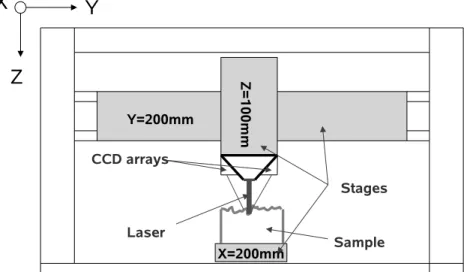
To get a fast and precise topography measurement of the fracture surfaces, we used an optical profiler (see Fig. 1) (M´eheust, 2002; Renard et al., 2004). The instrument provides a height measurement without any contact of the surface which allows a fast on-flight acquisition of the topography (up to 70 points per second). However this technique requires not to measure the original fracture butt a cast of the fracture made of an optically homogeneous material. To do
Fig. 1. Sketch of the optical profiler. The laser sensor sends a laser beam of 30 µm in diameter normally to the surface and records diffuse reflection from two ccd arrays. Height is deduced from a triangulation estimate. The sensor is attached to the Z-axis which is vertical and moved horizontally by the Y-axis, over the sample. The X-axis is the second horizontal translation stage that moves the sample. Maximum range of each translation stage is explicited. Their mechanical resolution is 1µm.
this, we apply a blue silicon resin (RTV 1570) on the granite surface and turn it out after drying to get a perfect counter molding of the granite surface. The use of a silicon cast aims at suppressing optical artifacts that might come from significant variations of the reflectivity when passing different minerals along the granite surface. Indeed, the silicon is uniformly blue and rather equally diffusive providing a high quality measurement of the fracture morphology. Therefore very high resolution map of the fracture can be obtained.
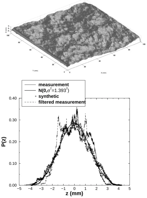
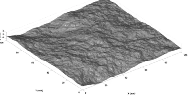
In the present study, a 3999×4000 image of the complete fracture surface is obtained with a vertical resolution of 2µm (see Fig. 2). The map consists of almost 16 millions pixels providing one of the highest image resolution ever obtained for a fracture surface. The mesh of the horizontal grid (i.e. along the (X,Y) plane) is 24µm×24µm and the total area is 95.952×95.976 mm2. A
mean plane estimated from a least square fit has been removed. The fracture surface shows a very rich distribution of asperities of any size (see the fractal dimension measured in Bouchaud et al. (1990) and the return probability measured in Schmittbuhl et al. (1995)), the aspect ratio of the asperities (i.e. height over lateral extension) being very small. To be more precise, an asperity can be defined as a connected surface entirely above the mean plane, the height of the asperity is the maximum z− coordinate of this surface, and its lateral extension refers to the x− or y− extent of the orthogonal projection of this surface on the mean plane.
−5 −4 −3 −2 −1 0 1 2 3 4 5 z (mm) 0.00 0.10 0.20 0.30 0.40 P(z) measurement N(0,σ2=1.3932) synthetic filtered measurement
Fig. 2. Top: 3D map of the silicon cast of a fresh granite fracture sampled with the optical profiler. The resolution of the map is 3999×4000 with a mesh of 24µm×24µm. On the left side of the image (low X), the initial machined notch is visible. Bottom: height distribution of the fracture topography. The best Gaus-sian fit for the whole distribution is plotted as: N (0, σ2) = (1/σ√2π) exp (−z2/2σ2) with σ = 1.393mm. Height distribution of the synthetic fracture topography pre-sented in Fig. 5 is added for comparison as the height distribution of the filtered measured surface shown in Fig. 8
2.2 Height statistics
The height distribution is computed and shown in Fig. 2. Even with a very large amount of data (i.e. 15996000 data points), the Gaussian fit obtained
from a least square fit, is a raw approximation. The rms of the Gaussian model provides an estimate of the height fluctuations: σ = 1.393 mm (see Fig. 2). An extended description of the height statistics, in particular the departure from a Gaussian statistics, is proposed in Santucci et al. (2006).
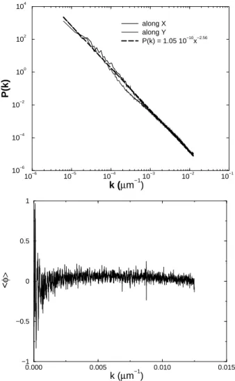
To characterize the possible spatial correlations of the height fluctuations, we computed the Fourier power spectrum of the topography P (k) = |˜z(k)|2 where
k is the wave number. This is also the Fourier transform of the height-height correlation: P (k) = ˜C(k) where C(δ) =< h(x)h(x + δ) >x − < h2 >x (see
Figure 3). A power law behavior is a good fit over more than 3 decades. The average phase spectrum < φ(k) > is also plotted in Figure 3. It shows the average over the y-axis of phase spectrum φ(kx) of profiles extracted along
x-axis. Phases almost average to zero for most wave numbers k showing their randomness. At low wave-numbers (i.e. low k), phases still show large fluc-tuations indicating that phases might be spatially correlated and not fully random.
2.3 Geometrical model
A self-affine surface is a possible geometrical model for roughness topogra-phies of fractures as shown in several previous studies (Brown and Scholz, 1985; Schmittbuhl et al., 1993, 1995; Bouchaud, 1997). Self-affinity is a scal-ing invariance property that reads as:
x → λx y → λy z → λζz (2)
where λ is a scaling factor and ζ is the roughness exponent. As can be seen from Eq (2), the scaling transformation is supposed to be isotropic within the mean plane (x, y) since the scaling factors are the same along x and y axes. Accordingly the fracture propagation direction is assumed not to influence the fracture roughness (M´eheust and Schmittbuhl, 2001; M´eheust, 2002). On the contrary, the scaling is anisotropic along the out of plane direction z. Indeed, the scaling factor is not the same along the mean plane (x, y) compared to the out of plane direction z. For the latter direction, the roughness exponent ζ describes how anisotropic is the property. When being equal to one, the prop-erty is isotropic and corresponds to a fractal. When the roughness exponent is different from one (i.e. classically between 0 and one, the scaling is anisotropic and the surface is self-affine.
10−6 10−5 10−4 10−3 10−2 10−1 k (µm−1) 10−6 10−4 10−2 100 102 104 P(k) along X along Y P(k) = 1.05 10−10x−2.56 0.000 0.005 0.010 0.015 k (µm−1) −1 −0.5 0 0.5 1 < φ>
Fig. 3. Top: Fourier spectra of the fracture morphology. Spectra are computed from 2D profiles extracted along either x or y direction (respectively parallel or perpen-dicular to the crack propagation) and then averaged over all the extracted profiles along the same direction (Schmittbuhl et al., 1995). The best power law fit is given: P (k) = 1.05 ·10−10x−2.56 with P (k) in µm3 (error bars are 5 ·10−11 for the prefactor
and 0.05 for the exponent). Bottom: Phase spectra have been computed along the X-direction and averaged over the Y-direction. Phases are qualitatively distributed randomly.
If a surface z(x, y) shows such a self-affine behavior, it can be shown that its 1D Fourier power spectrum fulfils the relation (Schmittbuhl et al., 1995): P (k) ∝ k−1−2ζ and the phase spectrum is supposed to be flat and
uncorre-lated. Figure 3 shows how good is the self-affine model for a high resolution measurement of a fracture surface. The estimate of the roughness exponent from a Fourier method, is ζ ≈ 0.78.
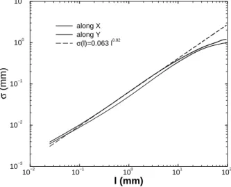
The self-affine property is also visible in the real space when computing the rms of the height fluctuations over a variable length scale l:
10−2 10−1 100 101 102 l (mm) 10−3 10−2 10−1 100 101 σ (mm) along X along Y σ(l)=0.063 l0.82
Fig. 4. Scaling of the rms σ(l) of the fracture topography along x- and y-axis. The best fit of the form σ(l) = l1−ζr lζ defines the roughness exponent ζ ≈ 0.82 and the
topothesy lr ≈ 2 · 10−7mm.
Figure 4 shows the scaling of the rms of the experimental surface. A self-affine surface shows a scaling of the second moment as: σ(l) = l1−ζ
r lζ where the
prefactor lrdefines the topothesy of the surface. We estimated lr ≈ 2·10−7mm
which is very small. The topothesy corresponds physically to the length scale for which the slope of the surface is one: σ(lr) = lr (Simonsen et al., 2000).
Accordingly the local slope of the surface is always significantly smaller than one for the range of scales that we explored, i.e. from 0.03 to 100 mm, as shown on Fig. 4.
2.4 Synthetic fracture surfaces
The knowledge of the roughness exponent and the topothesy allows the nu-merical construction of synthetic surfaces (Adler and Thovert, 1999; M´eheust and Schmittbuhl, 2001). Indeed, from the Fourier transform ˜R(k) of a ran-dom field or white noise of magnitude l1−ζ
r , it is possible to apply a fractional
integration in the Fourier domain by multiplying the Fourier transform by the wavenumber to the power −1 − ζ: ˜h(k) = k−1−ζR(k) and get a synthetic˜
fracture surface after applying an inverse Fourier transform.
Figure 5 shows an example of a synthetic surface of size 512×512 with compa-rable statistical parameters to the measured surface. The height distribution of it is shown in Fig. 2. Mean and root mean square are equal to those of the measured surface.
Fig. 5. Synthetic fracture surface (512 × 512) with a roughness exponent ζ = 0.82 and a topothesy lr= 2 · 10−7mm.
3 Numerical modeling of a viscous flow
3.1 Stokes flow
As mentioned in the introduction, we limit our study to viscous flow. Extension of the present work to higher Reynolds number will be addressed by a future work.
To study the viscous flow in a rough fracture, we developed a numerical simu-lation based on the Stokes equation (M´eheust and Schmittbuhl, 2001, 2003). As mentioned earlier, the rough aperture is considered as the void between a rough fracture surface a facing flat plane. In such a case, the height fluctuations of the fracture surface are identical to that of the aperture:
a(x, y) = Z(x, y) = z(x, y) + am (4)
where Z(x, y) is the height measurement of the topography in the reference frame of the upper flat plane and z(x, y) is the height fluctuations of zero mean (< z(x, y) >f racture= 0) and am is the so-called mechanical aperture which
corresponds to the average aperture of the fracture: < a(x, y) >f racture= am.
As shown in several studies (Adler and Thovert, 1999; M´eheust and Schmit-tbuhl, 2001), if the local aperture a(x, y) is slowly varying (i.e. ∂xa 1), the
lubrication approximation is valid. As a consequence, a local cubic law holds for the local flow rate:
q(x, y) = −a(x, y)
3
where q(x, y) = R
a(x,y)v(x, y, z)dz and v(x, y, z) is the local fluid velocity. In
doing so, the problem becomes two dimensional. It can be shown that the local flow rate is conservative: ∇ · q = 0 which leads to the Reynolds equation that is numerically solved:
∇ · a(x, y)
3
12η ∇P
!
= 0 (6)
The pressure field is solved using a finite difference scheme (M´eheust and Schmittbuhl, 2001) and a bi-conjugated gradient method for the matrix inver-sion (Press et al., 1992). The pressure field P (x, y) is described on grid twice coarser than the aperture field a(x, y). We reduce the resolution of the mea-sured aperture field to a 1000x1000 resolution by under-sampling because of numerical limitations which slightly reduces the scaling range of the aperture but has no influence on the self-affine property of it. Boundary conditions are defined as follow: a pressure drop ∆P is imposed along the x-axis between the inlet and outlet while no flux exists through the lateral boundaries.
The result of the simulation in terms of modulus of the local flux |q(x, y)| for am = acm is shown in Figure 6. The critical mechanical aperture acm is defined
as the smallest mechanical aperture to get only the highest asperity of the rough fracture surface in rigid contact to the facing plane. For the measured rough fracture, ac
m = 3.37 mm. This value could be high in comparison to the
in situ conditions of the Soultz-sous-Forˆets deep fractures.
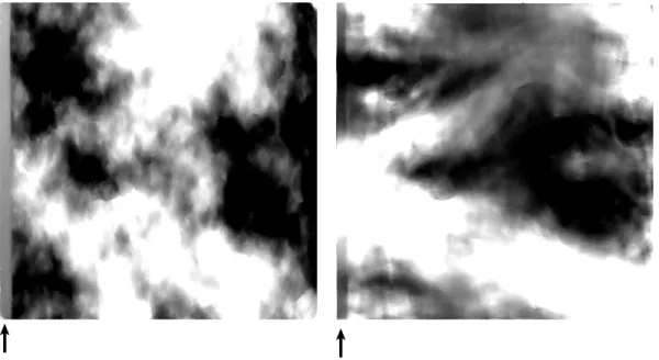
Figure 6 compares the aperture fluctuations to the local flux fluctuations. Both sub-images differ in their general aspect: aperture fluctuations show a rich, long range correlated, but isotropic pattern (M´eheust and Schmittbuhl, 2001). On the contrary, flux patches are anisotropic and a channeling effect is clearly visible. It is of interest to note that the region of maximum aperture on the upper side of the picture does not correspond to a maximum of the local flux. This shows the importance of large scale properties of the aperture to get extended channel where most of the flux takes place.
We also computed the hydraulic conductivity of the fracture as: K = ηQ/∆P since the system is square (Lx = Ly). If a cubic law were holding at large scale
for any aperture of the fracture, we would expect the hydraulic conductivity to behave as: K = a3
m/12 where am is the mechanical aperture. To check the
validity of such a large scale cubic law, we plotted in Figure 7 the ratio 12K/a3 m
which should be equal to one for a perfect cubic law. A significant departure from the cubic law is observed at small closure of the fracture (am ≈ acm).
Influence of the pressure drop orientation has been explored in M´eheust and Schmittbuhl (2001, 2003).
Fig. 6. Left: Gray level image of the fracture aperture (white corresponds to large aperture). Right: gray level map of the modulus of the local flux |q(x, y)| (white is for large flux). The global imposed flux is from left to right. The notch is visible on the left side of the images and marked by an arrow.
0 0.01 0.02 0.03 am (m) 0.7 0.8 0.9 1 K/(a m 3 /12)
Fig. 7. Ratio of the hydraulic conductivity K and expected hydraulic conductivity from a cubic law a3m/12 as a function of the mechanical aperture am. The vertical
dashed line indicates the aperture at rigid contact ac m.
3.2 Dominant role of large scale asperities
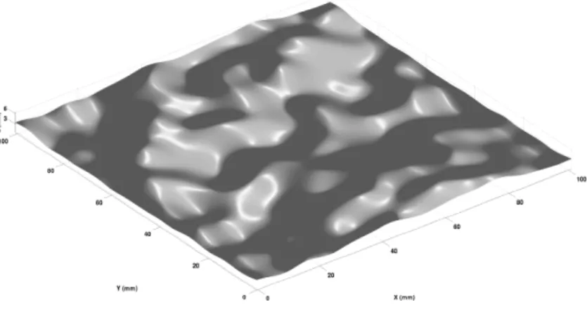
In comparison to an experimental approach, the numerical modelling allows to study explore with a new path, the role of the fracture roughness on the fluid flow. Indeed, it is possible to show that long wavelength modes of the aperture fluctuations are controlling the fluid flux. For this purpose we artificially
fil-Fig. 8. Example of a low-pass filter applied to the experimental surface. The cut-off frequency is kc/kmin = 8 which corresponds to 8 Fourier modes. The height
distribution of the surface is shown in Fig. 2.
tered the aperture field and studied the impact of the filtering on the hydraulic conductivity of the fracture. The filter is applied in the Fourier domain as a low-pass filter. Each modulus of the Fourier transform of the experimental aperture field that has a wavenumber k smaller than a cut-off wavenumber kc is set to zero. An inverse Fourier transform provides a smoothened
aper-ture field as illustrated in Fig 8 for kc = 8kmin where kmin is the smallest
wavenumber of the surface. Therefore only 8 Fourier modes in both directions kx and ky (i.e. 64 modes in total) are not equal to zero. Note that a direct
measurement with a poor spatial resolution could provide similar results but if it were done on a much larger sample to get a large statistics of the large wavenumber topography fluctuations.
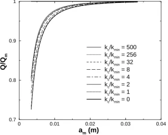
We then solve the Stokes equation and search for the evolution of the di-mensionless flux Q/Qm where Qm is the expected flux from the cubic law.
Figure 9 shows the effect of the filtering on the flux. It is of interest to see that already for kc = 2kmin (i.e. 2 Fourier modes in each direction) which is
a very smoothened version of the aperture field, most of the difference with the cubic law is obtained. Then increasing kc provides more and more details
of the full response kc= 500kmin. Accordingly, the knowledge of the aperture
does not need to be described with a high resolution but it has to be mea-sured on large wavelength. However, the exact value of the contact condition am = acm requires a very precise description of the highest asperity.
0 0.01 0.02 0.03 0.04 am (m) 0.7 0.8 0.9 1 Q/Q m kc/kmin = 500 kc/kmin = 256 kc/kmin = 32 kc/kmin = 8 kc/kmin = 4 kc/kmin = 2 kc/kmin = 1 kc/kmin = 0
Fig. 9. Evolution of the aperture filtering on the departure to the cubic law. The ratio of the flow rate and the flow rate deduced from the cubic law (Qm = a3m/12η ∆P )
as a function of the mechanical aperture. The aperture is filtered from a low-pass filter in the Fourier domain at k = kc. Only the two first Fourier modes of the
aperture field are responsible for most of the departure from the cubic law.
4 Experimental modelling
To check the validity of the Stokes equation to describe the flow in a rough fracture we conducted laboratory experiments that enable a direct check of the numerical results.
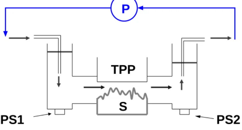
The experimental setup is described in Figure 10. It consists of a fracture permeameter where the fluid flux is imposed using a peristaltic pump in the range: 0-3 l/min (similar to the numerical simulations). Pressure difference between the inlet and outlet of the fracture is measured using two piezo-electric Honeywell 24PC sensors at the bottom of the input and output containers. The accuracy of the pressure measurement is 0.2 Pa (i.e. 0.02 mm of water). To get a stabilized measurement (no influence of the pump vibration), the pressure difference is sampled at a 1Hz frequency during 6 minutes. The pump is also run 15 minutes before any measurements to get a thermal equilibrium of the fluid.
In our setup, the mechanical aperture am is an adjustable parameter. It is
set with a precision of 0.25 mm. Indeed, a waterproof connection between the upper Plexiglas plate facing the rough fracture surface and the rest of the setup allows a vertical motion of the plate. Two bubble levels ensure parallel positions of the upper plate and the mean fracture plane. Indeed the mean fracture plane has been extracted from the roughness measurement and its crosses with the granite block boundaries, drawn on the block (with an angular resolution of 0.3 degree). A first bubble level is then attached to this
P
S
PS1
TPP
PS2
Fig. 10. Sketch of the experimental setup: fracture sample (S), transparent Plexiglas plate (TPP), peristaltic pump (P), pressure sensors (PS1, PS2).
mean fracture plane. A second bubble level is set on the upper Plexiglas plate. The comparison of the two bubble levels ensures the parallel position of the facing interfaces.
We chose a viscous fluid to be at low Reynolds number (i.e. laminar Stokes flow). Accordingly we used a glycerol/water mixture (90%/10%). Its density has been measured: ρ = 1200 kg/m3. The kinematic viscosity has also been
measured and its sensitivity to temperature: η(T ) ≈ 0.22 − 5.5 · 10−3T in
kg.m−1.s−1 with T in Celsius degree. These parameters are similar to those
used in the simulation.
As a first check of the Stokes flow, we checked the reversibility of the flow changing the flux direction for a given mechanical aperture am (see Figure 11
that shows the flux Q as a function of the pressure drop ∆P ). Twenty different values of the imposed flux are performed providing an accurate estimate of the relationship between flux and pressure drop. The reversibility is very good. It comes to excellent if the influence of the temperature on the viscosity is considered.
As a second check, we plotted similar quantities, Q versus ∆P , but for 10 different experiments for 5 apertures (2 experiments per aperture but changing the flow direction). We see that the linearity between the flux Q and the pressure drop ∆P is fulfilled over the range of explored fluxes. We also confirm the reversibility of the flow from the symmetry of the figures when changing the flow direction.
Finally we report the obtained ratio of the flux Q and the pressure drop ∆P as a function of the mechanical aperture (see Figure 13). Twenty four
exper-0 200 400 600 ∆P (Pa) 0 1e−05 2e−05 3e−05 Q (m 3 /s) + −
Fig. 11. Reversibility test: The flux Q is plotted versus the pressure drop ∆P be-tween the inlet and the outlet for the minimum possible aperture. Two set of ex-periments are reported: one for a direction of the flux labelled + and one for the opposite direction of the flux labelled −. No correction for the temperature varia-tion has been introduced though experiments were done with a 0.5◦C temperature
difference which correspond to a 3% difference in viscosity. Only the sign of the pressure drop has been changed for experiments in direction −.
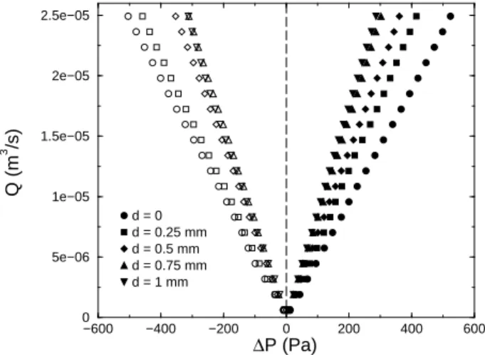
−600 −400 −200 0 200 400 600 ∆P (Pa) 0 5e−06 1e−05 1.5e−05 2e−05 2.5e−05 Q (m 3 /s) d = 0 d = 0.25 mm d = 0.5 mm d = 0.75 mm d = 1 mm
Fig. 12. Influence of the imposed shift d on the flow rate Q versus pressure drop ∆P behavior . For each mechanical aperture am = acm+ d, 20 steps of the imposed flux
have been performed (from 6.27 · 10−7 m3/s to 2.49 · 10−5 m3/s) in each direction
+ and −. Only experiments for d between 0 and 1 mm are reported here.
iments are reported. They were done with a relative error of the translation measurement of 0.25 mm. Since they are performed at slightly different tem-peratures, a temperature correction has been introduced using the measured temperature sensitivity of the viscosity to estimate the flux at the average temperature of 23.1◦C.
Experimental results show an increase of the ratio hydraulic conductivity Q/∆P (which is proportional to the hydraulic conductivity) for an increase of
0.002 0.004 0.006 0.008 0.010 am (m) 0 2e−07 4e−07 6e−07 8e−07 Q/ ∆ P Experiments Simulations
Fig. 13. Comparison between experiments and simulations: Evolution of the ratio of the flux |Q| and the pressure difference ∆P for 24 experiments. Experiments have a relative error for ac
m of 0.25 mm. The critical mechanical aperture obtained
from a contact test, has been found to be ac
m = 3.8 mm which is slightly higher
than the value obtained from the topography measurement ac
m = 3.37 (i.e. from the
measurement of the highest asperity). Simulations were performed for a viscosity η = 0.112 kg.m−1.s−1 to get a satisfactory match with absolute experimental data
(i.e. slightly higher than the experimentally measured values).
the mechanical aperture. At low mechanical aperture, experimental data (i.e. black circles in Figure 13) exhibit a clear trend and experiments at the same aperture but in opposite flow directions, show very consistent results. For com-parison, the results from numerical simulations are added in Figure 13. They are in good agreement with the experimental results despite the scattering of the experimental data. However the departure from the cubic law being of a small effect with the experimentally explored parameters and owing to the limited quality of the experimental data (i.e. too large error bar on the contact condition, ac
m), we could not observe clearly the departure as described in the
previous numerical section.
5 Conclusions
We measured the topography of a fresh fracture surface at very high resolution (almost 16 millions pixels). We confirmed that a self-affine model provides a nice description of the fracture geometry that can be used for many modellings where the fracture geometry might play a significant role: fluid flow, thermal advection and diffusion, chemical interaction like erosion or precipitation, ex-change surface measurement, etc.
Fracture roughness is shown to have a significant influence on the flow through its aperture. More precisely we show that only very large wavelengths of the
aperture fluctuations control most of the hydraulic conductivity in the limit of a viscous flow and a sufficiently open fracture. This observation suggests that only very coarse-grain measurement of the fracture aperture is required to describe the hydraulic fracture aperture. Indeed we show that only 4 modes of the Fourier transform of the aperture fluctuations account for most of the departure to the cubic law at small aperture. On the contrary, the knowledge of the mechanical aperture is very much controlled by the measurement of the largest asperities of the fracture topography. Unfortunately the later will be described by the tail of the topography distribution which requires a precise and intense geometrical characterization.
We thank Yves M´eheust, Gr´egor Duval, Am´elie Neuville and Samuel Mau-courant for fruitful discussions. The project has been supported by the Euro-pean EHDRA program and the french ECCO-PNRH program.
References
Adler, P., Thovert, J., 1999. Fractures and Fracture Networks. Kluwer aca-demic publishers, The Netherlands.
Bachler, D., Kohl, T., Rybach, L., 2003. Impact of graben-parallel faults on hydrothermal convection - rhine graben case study. Phys. Chem. Earth 28, 431–441.
Benderitter, Y., Elsass, P., 1995. Structural control of deep fluid circulation at the soultz hdr site, france: a review. Geotherm. Sci. Technol. 4 (4), 227–237. Bodin, J., Delay, F., de Marsily, G., 2003. Solute transport in a single fracture with negligible matrix permeability: 2. mathematical formalism. Hydrogeol. J. 11, 434–454.
Bouchaud, E., 1997. Scaling properties of cracks. J. Phys.: Cond. Matter 9, 4319–4344.
Bouchaud, E., Lapasset, G., Plan`es, J., 1990. Fractal dimension of fractured surfaces: a universal value ? Europhys. Lett. 13, 73–79.
Brown, S. R., 1987. Fluid flow through rock joints: the effect of surface rough-ness. J. Geophys. Res. 92, 1337–1347.
Brown, S. R., Scholz, C. H., 1985. Broad bandwidth study of the topography of natural rock surfaces. J. Geophys. Res. 90, 12575–12582.
Brush, D., Thomson, N., 2003. Fluid flow in synthetic rough-walled fractures: Navier-stokes, stokes, and local cubic law simulations. Water Resour. Res. 39 (4), 1085.
Evans, K., Genter, A., Sausse, J., 2005. Permeability creation and damage due to massive fluid injection into granite at 3.5 km at soultz: I. borehole observations. J. Geophys. Res. 110 (B04203), 0–19.
to mineral diagenesis in fractured crust: implications for hydrothermal cir-culation at mid-ocean ridges. Earth Planet. Sci. Lett. 184, 407–425.
Genter, A., Traineau, H., Led´esert, B., Bourgine, B., Gentier, S., June 10, 2000. Over 10 years of geological investigations within the hdr soultz project, france. In: Proceedings of the World Geothermal Congress 2000. Kyushu-Tohoku, pp. 3707–3712.
Glover, P. W. J., Matsuki, K., Hikima, R., Hayashi, K., 1998. Fluid flow in synthetic rough fractures and application to the hachimantai geomthermal hot rock test site. J. Geophys. Res. 103 (B5), 9621–9635.
Gutfraind, R., Hansen, A., 1995. Study of fracture permeability using lattice gas automata. Transp. Porous Media 18, 131–149.
Hakami, E., Larsson, E., 1996. Aperture mearurements and flow experiemnts on a single fracture. Int. J. Rock Mech. Min. Sci. & Geomech. Abstr. 33 (4), 395–404.
M´eheust, Y., 2002. ´Ecoulements dans les fractures ouvertes. Ph.D. thesis, Uni-versit´e Paris Sud.
M´eheust, Y., Schmittbuhl, J., 2000. Flow enhancement of a rough fracture. Geophys. Res. Lett. 27, 2989–2992.
M´eheust, Y., Schmittbuhl, J., 2001. Geometrical heterogeneities and perme-ability anisotropy of rough fractures. J. Geophys. Res. 106 (B2), 2089–2102. M´eheust, Y., Schmittbuhl, J., 2003. Scale effects related to flow in rough
frac-tures. PAGEOPH 160 (5-6), 1023–1050.
Murphy, H., 1979. Convective instabilites in vertical fractures and faults. J. Geophys. Res. 84 (B11), 6121–6130.
Neuman, S., 2005. Trends, prospects and challenges in quantifying flow and transport through fractured rocks. Hydrogeol. J. 13, 124–147.
Plourabou, F., Kurowski, P., Hulin, J., Roux, S., Schmittbuhl, J., 1995. Aper-ture of rough crack. Phys. Rev. E 51, 1675.
Press, W. H., Teukolsky, S. A., Vetterling, W. T., Flannery, B. P., 1992. Nu-merical Recipies. Cambridge University Press, New York.
Qian, J., Zhan, H., Zhao, W., Sun, F., 2005. Experimental study of turbulent unconfined groundwater flow in a single fracture. J. Hydrol. 311, 134–142. Renard, F., Schmittbuhl, J., Gratier, J. P., Meakin, P., Merino, E., 2004. The
three-dimensional roughness of stylolites in limestones. J. Geophys. Res. 109, 10.1029/2003JB002555.
Santucci, S., Mathiesen, J., M˚aløy, K. J., Hansen, A., Schmittbuhl, J., Vanel, L., Delaplace, A., Bakke, J. Ø. H., Ray, P., 2006. Statistics of fracture sur-faces, phys. Rev. E, revised.
Schmittbuhl, J., Chambon, G., Hansen, A., M.Bouchon, 2006. Are stress dis-tributions along faults the signature of asperity squeeze? Geophys. Rev. Lett. 33, L13307.
Schmittbuhl, J., Gentier, S., Roux, S., 1993. Field measurements of the rough-ness of fault surfaces. Geophys. Res. Lett. 20, 639–641.
Schmittbuhl, J., Schmitt, F., Scholz, C., 1995. Scaling invariance of crack surfaces. J. Geophys. Res. 100, 5953–5973.
Simonsen, I., Vandembroucq, D., Roux, S., 2000. Wave scattering from self-affine surfaces. Phys. Rev. E 61, 5914–5917.
Tournier, C., Genthon, P., Rabinowicz, M., 2000. The onset of natural con-vection in vertical fault planes: consequences for the thermal regime in cristalline basements and for heat recovery experiments. Geophys. J. Int. 140, 500–508.
Zhao, C., Hobbs, B., M¨uhlhaus, H., Ord, A., Lin, G., 2003. Convective in-stability of 3-d fluid saturated geological fault zones heated from below. Geophys. J. Int. 155, 213–220.