HAL Id: hal-00302672
https://hal.archives-ouvertes.fr/hal-00302672
Submitted on 9 Nov 2005
HAL is a multi-disciplinary open access
archive for the deposit and dissemination of
sci-entific research documents, whether they are
pub-lished or not. The documents may come from
teaching and research institutions in France or
abroad, or from public or private research centers.
L’archive ouverte pluridisciplinaire HAL, est
destinée au dépôt et à la diffusion de documents
scientifiques de niveau recherche, publiés ou non,
émanant des établissements d’enseignement et de
recherche français ou étrangers, des laboratoires
publics ou privés.
J. R. Holliday, K. Z. Nanjo, K. F. Tiampo, J. B. Rundle, D. L. Turcotte
To cite this version:
J. R. Holliday, K. Z. Nanjo, K. F. Tiampo, J. B. Rundle, D. L. Turcotte. Earthquake forecasting and
its verification. Nonlinear Processes in Geophysics, European Geosciences Union (EGU), 2005, 12 (6),
pp.965-977. �hal-00302672�
SRef-ID: 1607-7946/npg/2005-12-965 European Geosciences Union
© 2005 Author(s). This work is licensed under a Creative Commons License.
Nonlinear Processes
in Geophysics
Earthquake forecasting and its verification
J. R. Holliday1,2, K. Z. Nanjo3,2, K. F. Tiampo4, J. B. Rundle2,1, and D. L. Turcotte5 1Department of Physics, University of California, Davis, USA
2Computational Science and Engineering Center, University of California, Davis, USA 3The Institute of Statistical Mathematics, Tokyo, Japan
4Department of Earth Sciences, University of Western Ontario, Canada 5Geology Department, University of California, Davis, USA
Received: 8 August 2005 – Revised: 12 October 2005 – Accepted: 19 October 2005 – Published: 9 November 2005
Abstract. No proven method is currently available for the
reliable short time prediction of earthquakes (minutes to months). However, it is possible to make probabilistic haz-ard assessments for earthquake risk. In this paper we discuss a new approach to earthquake forecasting based on a pattern informatics (PI) method which quantifies temporal variations in seismicity. The output, which is based on an association of small earthquakes with future large earthquakes, is a map of areas in a seismogenic region (“hotspots”) where earth-quakes are forecast to occur in a future 10-year time span. This approach has been successfully applied to California, to Japan, and on a worldwide basis. Because a sharp decision threshold is used, these forecasts are binary–an earthquake is forecast either to occur or to not occur. The standard ap-proach to the evaluation of a binary forecast is the use of the relative (or receiver) operating characteristic (ROC) diagram, which is a more restrictive test and less subject to bias than maximum likelihood tests. To test our PI method, we made two types of retrospective forecasts for California. The first is the PI method and the second is a relative intensity (RI) forecast based on the hypothesis that future large earthquakes will occur where most smaller earthquakes have occurred in the recent past. While both retrospective forecasts are for the ten year period 1 January 2000 to 31 December 2009, we performed an interim analysis 5 years into the forecast. The PI method out performs the RI method under most circum-stances.
1 Introduction
Earthquakes are the most feared of natural hazards because they occur without warning. Hurricanes can be tracked, floods develop gradually, and volcanic eruptions are pre-ceded by a variety of precursory phenomena. Earthquakes, however, generally occur without any warning. There have Correspondence to: J. R. Holliday
been a wide variety of approaches applied to the forecast-ing of earthquakes (Mogi, 1985; Turcotte, 1991; Lomnitz, 1994; Keilis-Borok, 2002; Scholz, 2002; Kanamori, 2003). These approaches can be divided into two general classes; the first is based on empirical observations of precursory changes. Examples include precursory seismic activity, pre-cursory ground motions, and many others. The second ap-proach is based on statistical patterns of seismicity. Neither approach has been able to provide reliable short-term fore-casts (days to months) on a consistent basis.
Although short-term predictions are not available, long-term seismic-hazard assessments can be made. A large frac-tion of all earthquakes occur in the vicinity of plate bound-aries, although some do occur in plate interiors. It is also possible to assess the long-term probability of having an earthquake of a specified magnitude in a specified region. These assessments are primarily based on the hypothesis that future earthquakes will occur in regions where past earth-quakes have occurred (Frankel, 1995; Kossobokov et al., 2000). Specifically, the rate of occurrence of small earth-quakes in a region can be analyzed to assess the probability of occurrence of much larger earthquakes.
The principal focus of this paper is a new approach to earthquake forecasting (Rundle et al., 2002; Tiampo et al., 2002b,a; Rundle et al., 2003; Appendix C). Our method does not predict the exact times and locations of earthquakes, but it does forecast the regions (hotspots) where earthquakes are most likely to occur in the relatively near future (typ-ically ten years). The objective is to reduce the areas of earthquake risk relative to those given by long-term hazard assessments. Our approach is based on pattern informatics (PI), a technique that quantifies temporal variations in seis-micity patterns. The result is a map of areas in a seismogenic region (hotspots) where earthquakes are likely to occur dur-ing a specified period in the future. A forecast for California was published by our group in 2002 (Rundle et al., 2002). Subsequently, sixteen of the eighteen California earthquakes with magnitudes M≥5 occurred in or immediately adjacent to the resulting hotspots. A forecast for Japan, presented in
Tokyo in early October 2004, successfully forecast the loca-tion of the M=6.8 Niigata earthquake that occurred on 23 October 2004. A global forecast, presented at the early De-cember 2004 meeting of the American Geophysical Union, successfully forecast the locations of the 23 December 2004, M=8.1 Macquarie Island earthquake, and the 26 December 2004 M=9.0 Sumatra earthquake. Before presenting further details of these studies we will give a brief overview of the current state of earthquake prediction and forecasting.
2 Empirical approaches
Empirical approaches to earthquake prediction rely on lo-cal observations of some type of precursory phenomena. In the near vicinity of the earthquake to be predicted, it has been suggested that one or more of the following phenom-ena may indicate a future earthquake (Mogi, 1985; Turcotte, 1991; Lomnitz, 1994; Keilis-Borok, 2002; Scholz, 2002; Kanamori, 2003): 1) precursory increase or decrease in seis-micity in the vicinity of the origin of a future earthquake rupture, 2) precursory fault slip that leads to surface tilt and/or displacements, 3) electromagnetic signals, 4) chem-ical emissions, and 5) changes in animal behavior. Similarly, it has been suggested that precursory increases in seismic activity over large regions may indicate a future earthquake as well (Prozoroff, 1975; Dobrovolsky et al., 1979; Keilis-Borok et al., 1980; Press and Allen, 1995).
Examples of successful near-term predictions of future earthquakes have been rare. A notable exception was the prediction of the M=7.3 Haicheng earthquake in northeast China that occurred on 4 February 1975. This prediction led to the evacuation of the city which undoubtedly saved many lives. The Chinese reported that the successful prediction was based on foreshocks, groundwater anomalies, and an-imal behavior. Unfortunately, a similar prediction was not made prior to the magnitude M=7.8 Tangshan earthquake that occurred on 28 July 1976 (Utsu, 2003). Official reports placed the death toll in this earthquake at 242 000, although unofficial reports placed it as high as 655 000.
In order to thoroughly test for the occurrence of direct pre-cursors the United States Geological Survey (USGS) initi-ated the Parkfield (California) Earthquake Prediction Exper-iment in 1985 (Bakun and Lindh, 1985; Kanamori, 2003). Earthquakes on this section of the San Andreas had occurred in 1857, 1881, 1901, 1922, 1934, and 1966. It was expected that the next earthquake in this sequence would occur by the early 1990’s, and an extensive range of instrumentation was installed. The next earthquake in the sequence finally oc-curred on 28 September 2004. No precursory phenomena were observed that were significantly above the background noise level. Although the use of empirical precursors cannot be ruled out, the future of those approaches does not appear to be promising at this time.
3 Statistical and statistical physics approaches
A variety of studies have utilized variations in seismicity over relatively large distances to forecast future earthquakes. The distances are large relative to the rupture dimension of the subsequent earthquake. These approaches are based on the concept that the earth’s crust is an activated thermodynamic system (Rundle et al., 2003). Among the evidence for this be-havior is the continuous level of background seismicity in all seismographic areas. About a million magnitude two earth-quakes occur each year on our planet. In southern Califor-nia about a thousand magnitude two earthquakes occur each year. Except for the aftershocks of large earthquakes, such as the 1992 M=7.3 Landers earthquake, this seismic activity is essentially constant over time. If the level of background seismicity varied systematically with the occurrence of large earthquakes, earthquake forecasting would be relatively easy. This, however, is not the case.
There is increasing evidence that there are systematic pre-cursory variations in some aspects of regional seismicity. For example, it has been observed that there is a systematic vari-ation in the number of magnitude M=3 and larger earth-quakes prior to at least some magnitude M=5 and larger earthquakes, and a systematic variation in the number of magnitude M=5 and larger earthquakes prior to some mag-nitude M=7 and larger earthquakes. The spatial regions as-sociated with this phenomena tend to be relatively large, sug-gesting that an earthquake may resemble a phase change with an increase in the “correlation length” prior to an earthquake (Bowman et al., 1998; Jaum´e and Sykes, 1999). There have also been reports of anomalous quiescence in the source re-gion prior to a large earthquake, a pattern that is often called a “Mogi Donut” (Mogi, 1985; Kanamori, 2003; Wyss and Habermann, 1988; Wyss, 1997).
Many authors have noted the occurrence of a relatively large number of intermediate-sized earthquakes (foreshocks) prior to a great earthquake. A specific example was the se-quence of earthquakes that preceded the 1906 San Francisco earthquake (Sykes and Jaum´e, 1990). This seismic activa-tion has been quantified as a power law increase in seismicity prior to earthquakes (Bowman et al., 1998; Jaum´e and Sykes, 1999; Bufe and Varnes, 1993; Bufe et al., 1994; Brehm and Braile, 1998, 1999; Main, 1999; Robinson, 2000; Bowman and King, 2001; Yang et al., 2001; King and Bowman, 2003; Bowman and Sammis, 2004; Sammis et al., 2004). Unfortu-nately the success of these studies has depended on knowing the location of the subsequent earthquake.
A series of statistical algorithms to make intermediate term earthquake predictions have been developed by a Russian group under the direction of V. I. Keilis-Borok using pattern recognition techniques (Keilis-Borok, 1990, 1996). Seismic-ity in various circular regions was analyzed. Based primar-ily on seismic activation, earthquake alarms were issued for one or more regions, with the alarms generally lasting for five years. Alarms have been issued regularly since the mid 1980’s and scored two notable successes: the prediction of the 1988 Armenian earthquake and the 1989 Loma Prieta
earthquake. While a reasonably high success rate has been achieved, there have been some notable misses including the recent M=9.0 Sumatra and M=8.1 Macquerie Island earth-quakes.
More recently, this group has used chains of premoni-tory earthquakes as the basis for issuing alarms (Shebalin et al., 2004; Keilis-Borok et al., 2004). This method success-fully predicted the M=6.5, 22 December 2003 San Simeon (California) earthquake and the M=8.1, 25 September 2003 Tokachi-oki, (Japan) earthquake with lead times of six and seven months respectively. However, an alarm issued for southern California, valid during the spring and summer of 2004, was a false alarm.
4 Chaos and forecasting
Earthquakes are caused by displacements on preexisting faults. Most earthquakes occur at or near the boundaries be-tween the near-rigid plates of plate tectonics. Earthquakes in California are associated with the relative motion between the Pacific plate and the North American plate. Much of this motion is taken up by displacements on the San An-dreas fault, but deformation and earthquakes extend from the Rocky Mountains on the east into the Pacific Ocean adjacent to California on the west. Clearly this deformation and the associated earthquakes are extremely complex.
Slider-block models are considered to be simple analogs to seismicity. A pair of interacting slider-blocks have been shown to exhibit classical chaotic behavior (Turcotte, 1997). This low-order behavior is taken to be evidence for the chaotic behavior of seismicity in the same way that the chaotic behavior of the low-order Lorentz equations is taken as evidence for the chaotic behavior of weather and climate. Some authors (Geller et al., 1997; Geller, 1997) have argued that this chaotic behavior precludes the prediction of earth-quakes. However, weather is also chaotic, but forecasts can be made. Weather forecasts are probabilistic in the sense that weather cannot be predicted exactly. One such example is the track of a hurricane. Probabilistic forecasts of hurricane tracks are routinely made; sometimes they are extremely ac-curate while at other times they are not. Another example of weather forecasting is the forecast of El Ni˜no events. Fore-casting techniques based on pattern recognition and principle components of the sea surface temperature fluctuation time series have been developed that are quite successful in fore-casting future El Ni˜nos, but again they are probabilistic in nature (Chen et al., 2004). It has also been argued (Sykes et al., 1999) that chaotic behavior does not preclude the prob-abilistic forecasting of future earthquakes. Over the past five years our group has developed (Rundle et al., 2002; Tiampo et al., 2002b,a; Rundle et al., 2003; Holliday et al., 2005a) a technique for forecasting the locations where earthquakes will occur based on pattern informatics (PI). This type of approach has close links to principle component analysis, which has been successfully used for the forecasting of El Ni˜nos.
5 The PI method
Seismic networks provide the times and locations of earth-quakes over a wide range of scales. One of the most sensitive networks has been deployed over southern California and the resulting catalog is readily available. Our objective has been to analyze the historical seismicity for anomalous behavior that would provide information on the occurrence of future earthquakes. At this point we are not able to forecast the times of future earthquakes with precision. However, our ap-proach does appear to select the regions where earthquakes are most likely to occur during a future time window. At the present time, this time window is typically taken to be ten years, although it appears that it is possible to utilize shorter time windows.
Our approach divides the seismogenic region to be stud-ied into a grid of square boxes whose size is related to the magnitude of the earthquakes to be forecast. The rates of seismicity in each box are studied to quantify anomalous be-havior. The basic idea is that any seismicity precursors rep-resent changes, either a local increase or decrease of seismic activity, so our method identifies the locations in which these changes are most significant during a predefined change in-terval. The subsequent forecast interval is the decadal time window during which the forecast is valid. The box size is se-lected to be consistent with the size of the earthquakes being forecasted (Bowman et al., 1998), and the minimum earth-quake magnitude considered is the lower limit of sensitivity and completeness of the network in the region under consid-eration.
While a detailed explanation of the PI method that we have used for earthquake forecasting is included in Appendix A, a compact utilization is given as follows:
1. The region of interest is divided into NB square boxes
with linear dimension 1x. Boxes are identified by a subscript i and are centered at xi. For each box, there is
a time series Ni(t ), which is the instantaneous number
of earthquakes per unit time at time t larger than the lower cut-off magnitude Mc. The time series in box i is
defined between a base time tband the present time t .
2. All earthquakes in the region of interest with magni-tudes greater than a lower cutoff magnitude Mcare
in-cluded. The lower cutoff magnitude Mc is specified in
order to ensure completeness of the data through time, from an initial time t0to a final time t2.
3. Three time intervals are considered: (a) A reference time interval from tbto t1.
(b) A second time interval from tb to t2, t2>t1. The change interval over which seismic activity changes are determined is then t2−t1. The time tbis chosen
to lie between t0and t1. Typically we take t0=1932, t1=1990, and t2=2000. The objective is to quantify anomalous seismic activity in the change interval t1 to t2relative to the reference interval tbto t1.
(c) The forecast time interval t2 to t3, for which the forecast is valid. We take the change and forecast intervals to have the same length. For the above example, t3=2010.
4. The seismic intensity in box i, Ii(tb, t ), between two
times tb<t, can then be defined as the average number
of earthquakes with magnitudes greater than Mcthat
oc-cur in the box per unit time during the specified time in-terval tbto t . Therefore, using discrete notation, we can
write: Ii(tb, t ) = 1 t − tb t X t0=t b Ni(t0), (1)
where the sum is performed over increments of the time series, say days.
5. In order to compare the intensities from different time intervals, we require that they have the same statistical properties. We therefore normalize the seismic intensi-ties by subtracting the mean seismic activity of all boxes and dividing by the standard deviation of the seismic ac-tivity in all boxes. The statistically normalized seismic intensity of box i during the time interval tbto t is then
defined by ˆ Ii(tb, t ) = Ii(tb, t )− < I (tb, t ) > σ (tb, t ) , (2)
where < I (tb, t )>is the mean intensity averaged over
all the boxes and σ (tb, t )is the standard deviation of
intensity over all the boxes.
6. Our measure of anomalous seismicity in box i is the dif-ference between the two normalized seismic intensities: 1Ii(tb, t1, t2) = ˆIi(tb, t2) − ˆIi(tb, t1). (3) This measure is motivated by the assumption of pure phase dynamics (Rundle et al., 2000a,b) that important changes in seismicity will be given by the change in the anomalous seismicity over time.
7. To reduce the relative importance of random fluctua-tions (noise) in seismic activity, we compute the average change in intensity, 1Ii(t0, t1, t2)over all possible pairs
of normalized intensity maps having the same change interval: 1Ii(t0, t1, t2) = 1 t1−t0 t1 X tb=t0 1Ii(tb, t1, t2), (4)
where the sum is performed over increments of the time series, which here are days.
8. We hypothesize that the probability of a future earth-quake in box i, Pi(t0, t1, t2, ), is proportional to the
square of the average intensity change: Pi(t0, t1, t2, ) ∝ 1Ii(tb, t1, t2)
2
. (5)
The constant of proportionality can be determined by re-quiring unit probability but is not important to the anal-ysis.
9. To identify anomalous regions, we wish to compute the change in the probability Pi(t0, t1, t2, ) relative to the background so that we subtract the mean probability over all boxes. We denote this change in the probability by
1Pi(t0, t1, t2) = Pi(t0, t1, t2)− < Pi(t0, t1, t2) >, (6) where <Pi(t0, t1, t2)>is the background probability for a large earthquake.
Hotspots are defined to be the regions where 1Pi(t0, t1, t2) is positive. In these regions, Pi(t0, t1, t2)is larger than the average value for all boxes (the background level). Note that since the intensities are squared in defining probabilities the hotspots may be due to either increases of seismic activity during the change time interval (activation) or due to decreases (quiescence). We hypothesize that earthquakes with magnitudes larger than Mc+2 will occur
preferentially in hotspots during the forecast time interval t2 to t3.
6 Applications of the PI method
The PI method was first applied to seismicity in southern California and adjacent regions (32◦ to 37◦N lat, 238◦ to 245◦E long). This region was divided into a grid of 3500 boxes with 1x=0.1◦ (11 km). Consistent with the sensi-tivity of the southern California seismic network, the lower magnitude cutoff was taken to be M=3. The initial time was t0=1932, the change interval was from t1=1990 to t2=2000, and the forecast interval was from t2=2000 to t3=2010. The initial studies for California were published in 2002 (Rundle et al., 2002), the results are reproduced in Fig. 1. The col-ored regions are the hotspots defined to be the boxes where 1P is positive. This forecast of where earthquakes would likely occur was considered to be valid for the forecast in-terval from 2000 to 2010 and would be applicable for earth-quakes with M=5 and larger. Since 1 January 2000, eighteen significant earthquakes have occurred in the test region. We consider a significant earthquake to be an event that was ini-tially assigned a magnitude 5 or larger. These are also shown in Fig. 1, and information on these earthquakes is given in Table 1. We consider the forecast to be successful if the epi-center of the earthquake lies within a hotspot box or in one of the eight adjoining boxes (Moore, 1962). Sixteen of the eighteen earthquakes were successfully forecast.
-4 -3 -2 -1 0 log ( ∆P / ∆Pmax ) -123˚ -122˚ -121˚ -120˚ -119˚ -118˚ -117˚ -116˚ -115˚ 32˚ 33˚ 34˚ 35˚ 36˚ 37˚ 38˚
Fig. 1. Application of the PI method to southern California.
Col-ored areas are the forecast hotspots for the occurrence of M≥5 earthquakes during the period 2000-2010 derived using the PI method. The color scale gives values of the log10(P /Pmax). Also shown are the locations of the eighteen earthquakes with M≥5 that have occurred in the region since 1 January 2000. Sixteen of the eighteen earthquakes were successfully forecast. More details of the earthquakes are given in Table 1.
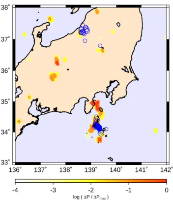
The second area to which the PI method was applied was Japan. The forecast hotspots for the Tokyo region (33◦ to
38◦N lat, 136◦ to 142◦W long) are given in Fig. 2. The
initial time was t0=1965, and the change and forecast inter-vals were the same as those used for California. Between 1 January 2000 and 14 October 2004, 99 earthquakes occurred and 91 earthquakes were successfully forecast. This forecast was presented at the International Conference on Geodynam-ics, 14–16 October 2004, Tokyo by one of the authors (JBR). Subsequently the Niigata earthquake (M=6.8) occurred on 23 October 2004. This earthquake and its subsequent M≥5 aftershocks were successfully forecast.
The PI method has also been applied on a worldwide basis. In this case 1◦×1◦ boxes were considered, 1x=1◦
(110 km). Consistent with the sensitivity of the global seis-mic network the lower magnitude cutoff was taken to be Mc =5. The initial time was t0=1965; the change and fore-cast intervals were the same as above. The resulting map of hotspots was presented by two of the authors (DLT and JRH) at the Fall Meeting of the American Geophysical Union on 14 December 2004 (abstracts: AGUF2004NG24B-01 and AGUF2004NG54A-08). This map is given in Fig. 3. This forecast of where earthquakes would occur was considered to be valid for the period 2000 to 2010 and would be ap-plicable for earthquakes with magnitudes greater than 7.0.
Table 1. Earthquakes with M≥5 that occurred in the California test
region since 1 January 2000. Sixteen of these eighteen earthquakes were successfully forecast. The two missed events are marked with an asterisk.
Event Magnitude Local Time
1 Big Bear I M=5.1 10 Feb. 2001
2 Coso M=5.1 17 July 2001
3 Anza I M=5.1 31 Oct. 2001
4 Baja M=5.7 22 Feb. 2002
5 Gilroy M=5.0 14 May 2002
6 Big Bear II M=5.4 22 Feb. 2003
7 San Simeon? M=6.5 22 Dec. 2003
8 San Clemente Island? M=5.2 15 June 2004
9 Bodie I M=5.5 18 Sep. 2004
10 Bodie II M=5.4 18 Sep. 2004
11 Parkfield I M=6.0 28 Sep. 2004
12 Parkfield II M=5.2 29 Sep. 2004
13 Arvin M=5.0 29 Sep. 2004
14 Parkfield III M=5.0 30 Sep. 2004
15 Wheeler Ridge M=5.2 16 April 2005
16 Anza II M=5.2 12 June 2005
17 Yucaipa M=4.9 16 June 2005
18 Obsidian Butte M=5.1 2 Sep. 2005
Between 1 January 2000 and 14 December 2004 there were sixty eight M≥7 earthquakes worldwide; fifty seven of these earthquakes occurred within a hotspot or adjoining boxes. Subsequent to the meeting presentation, the M=8.1 Mac-quarie Island earthquake occurred on 23 December 2004 and the M=9.0 Sumatra earthquake occurred on 26 December 2004. The epicenters of both earthquakes were successfully forecast.
7 Forecast verification
Previous tests of earthquake forecasts have emphasized the likelihood test (Kagan and Jackson, 2000; Rundle et al., 2002; Tiampo et al., 2002b; Holliday et al., 2005a). These tests have the significant disadvantage that they are overly sensitive to the least probable events. For example, con-sider two forecasts. The first perfectly forecasts 99 out of 100 events but assigns zero probability to the last event. The second assigns zero probability to all 100 events. Under a log-likelihood test, both forecasts will have the same skill score of −∞. Furthermore, a naive forecast that assigns uni-form probability to all possible sites will always score higher than a forecast that misses only a single event but is otherwise superior. For this reason, likelihood tests are more subject to unconscious bias. Other methods of evaluating earthquake forecasts are suggested by Harte and Vere-Jones (2005) and Holliday et al. (2005b).
An extensive review on forecast verification in the atmo-spheric sciences has been given by Jolliffe and Stephenson (2003). The wide variety of approaches that they consider
-4 -3 -2 -1 0 log ( ∆P / ∆Pmax ) 136˚ 137˚ 138˚ 139˚ 140˚ 141˚ 142˚ 33˚ 34˚ 35˚ 36˚ 37˚ 38˚
Fig. 2. Application of the PI method to central Japan. Colored
areas are the forecast hotspots for the occurrence of M≥5 earth-quakes during the period 2000-2010 derived using the PI method. The color scale gives values of the log10(P /Pmax). Also shown are
the locations of the 99 earthquakes with M≥5 that have occurred in the region since 1 January 2000.
are directly applicable to earthquake forecasts as well. The earthquake forecasts considered in this paper can be viewed as binary forecasts by considering the events (earthquakes) as being forecast either to occur or not to occur in a given box. We consider that there are four possible outcomes for each box, thus two ways to classify each red, hotspot, box, and two ways to classify each white, non-hotspot, box:
1. An event occurs in a hotspot box or within the Moore neighborhood of the box (the Moore neighborhood is comprised of the eight boxes surrounding the forecast box). This is a success.
2. No event occurs in a white non-hotspot box. This is also a success.
3. No event occurs in a hotspot box or within the Moore neighborhood of the hotspot box. This is a false alarm. 4. An event occurs in a white, non-hotspot box that is not
within the Moore neighborhood of a hotspot box. This is a failure to forecast.
We note that these rules tend to give credit, as successful forecasts, for events that occur very near hotspot boxes. We have adopted these rules in part because the grid of boxes is positioned arbitrarily on the seismically active region, thus
-4 -3 -2 -1 0 log ( ∆P / ∆Pmax ) -30˚ 0˚ 30˚ 60˚ 90˚ 120˚ 150˚ 180˚ -150˚ -120˚ -90˚ -60˚ -30˚ -60˚ -60˚ -40˚ -40˚ -20˚ -20˚ 0˚ 0˚ 20˚ 20˚ 40˚ 40˚ 60˚ 60˚
Fig. 3. World-wide application of the PI method. Colored areas are
the forecast hotspots for the occurrence of M≥7 earthquakes during the period 2000-2010 derived using the PI method. The color scale gives values of the log10(P /Pmax). Also shown are the locations
of the sixty eight earthquakes with M≥7 that have occurred in the region since 1 January 2000.
we allow a margin of error of ±1 box dimension. In addi-tion, the events we are forecasting are large enough so that their source dimension approaches, and can even exceed, the box dimension meaning that an event might have its epicen-ter outside a hotspot box, but the rupture might then propa-gate into the box. Other similar rules are possible but we have found that all such rules basically lead to similar results.
The standard approach to the evaluation of a binary fore-cast is the use of a relative operating characteristic (ROC) di-agram (Swets, 1973; Mason, 2003). Standard ROC didi-agrams consider the fraction of failures-to-predict and the fraction of false alarms. This method evaluates the performance of the forecast method relative to random chance by constructing a plot of the fraction of failures to predict against the frac-tion of false alarms for an ensemble of forecasts. Molchan (1997) has used a modification of this method to evaluate the success of intermediate term earthquake forecasts.
The binary approach has a long history, over 100 years, in the verification of tornado forecasts (Mason, 2003). These forecasts take the form of a tornado forecast for a specific location and time interval, each forecast having a binary set of possible outcomes. For example, during a given time win-dow of several hours duration, a forecast is issued in which a list of counties is given with a statement that one or more tornadoes will or will not occur. A 2×2 contingency table is then constructed, the top row contains the counties in which tornadoes are forecast to occur and the bottom row contains counties in which tornadoes are forecast to not occur. Sim-ilarly, the left column represents counties in which torna-does were actually observed, and the right column represents counties in which no tornadoes were observed.
With respect to earthquakes, our forecasts take exactly this form. A time window is proposed during which the forecast of large earthquakes having a magnitude above some min-imum threshold is considered valid. An example might be a forecast of earthquakes larger than M=5 during a period
of five or ten years duration. A map of the seismically ac-tive region is then completely covered (“tiled”) with boxes of two types: boxes in which the epicenters of at least one large earthquake are forecast to occur and boxes in which large earthquakes are forecast to not occur. In other types of forecasts, large earthquakes are given some continuous prob-ability of occurrence from 0% to 100% in each box (Kagan and Jackson, 2000). These forecasts can be converted to the binary type by the application of a decision threshold. Boxes having a probability below the threshold are assigned a fore-cast rating of non-occurrence during the time window, while boxes having a probability above the threshold are assigned a forecast rating of occurrence. A high threshold value may lead to many failures to predict (events that occur where no event is forecast), but few false alarms (an event is forecast at a location but no event occurs). The level at which the deci-sion threshold is set is then a matter of public policy specified by emergency planners, representing a balance between the prevalence of failures to predict and false alarms.
8 Binary earthquake forecast verification
To illustrate this approach to earthquake forecast verification, we have constructed two types of retrospective binary fore-casts for California. The first type of forecast utilizes the PI method described above. We apply the method to southern California and adjacent regions (32◦to 38.3◦N lat, 238◦ to 245◦E long) using a grid of boxes with 1x=0.1◦and a lower magnitude cutoff Mc=3.0. For this retrospective forecast we
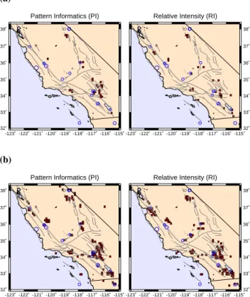
take the initial time t0=1932, the change interval t1=1989 to t2=2000, and the forecast interval t2=2000 to t3=2010 (Rundle et al., 2002; Tiampo et al., 2002b). In the analysis given above we considered regions with 1P positive to be hotspots. The PI forecast under the above conditions with 1P >0 is given in Fig. 4b. Hotspots include 127 of the 5040 boxes considered. This forecast corresponds to that given in Fig. 1. The threshold for hotspot activation can be varied by changing the threshold value for 1P . A forecast using a higher threshold value is given in Fig. 4a. Hotspots here include only 29 of the 5040 boxes considered.
An alternative approach to earthquake forecasting is to use the rate of occurrence of earthquakes in the past. We refer to this type of forecast as a relative intensity (RI) forecast. In such a forecast, the study region is tiled with boxes of size 0.1◦×0.1◦. The number of earthquakes with magnitude
M≥3.0 in each box down to a depth of 20 km is determined over the time period from t0=1932 to t2=2000. The RI score for each box is then computed as the total number of earth-quakes in the box in the time period divided by the value for the box having the largest value. A threshold value in the interval [0, 1] is then selected. Large earthquakes having M≥5 are then considered possible only in boxes having an RI value larger than the threshold. The remaining boxes with RI scores smaller than the threshold represent sites at which large earthquakes are forecast to not occur. The physical jus-tification for this type of forecast is that large earthquakes
(a)
Pattern Informatics (PI)
-123˚ -122˚ -121˚ -120˚ -119˚ -118˚ -117˚ -116˚ -115˚ 32˚ 33˚ 34˚ 35˚ 36˚ 37˚ 38˚
Relative Intensity (RI)
-123˚ -122˚ -121˚ -120˚ -119˚ -118˚ -117˚ -116˚ -115˚ 32˚ 33˚ 34˚ 35˚ 36˚ 37˚ 38˚ (b)
Pattern Informatics (PI)
-123˚ -122˚ -121˚ -120˚ -119˚ -118˚ -117˚ -116˚ -115˚ 32˚ 33˚ 34˚ 35˚ 36˚ 37˚ 38˚
Relative Intensity (RI)
-123˚ -122˚ -121˚ -120˚ -119˚ -118˚ -117˚ -116˚ -115˚ 32˚ 33˚ 34˚ 35˚ 36˚ 37˚ 38˚
Fig. 4. Retrospective application of the PI and RI methods for
southern California as a function of false alarm rate. Red boxes are the forecast hotspots for the occurrence of M≥5 earthquakes during the period 2000 to 2005. Also shown are the locations of the M≥5 earthquakes that occurred in this region during the forecast period. In (a), a threshold value was chosen such that F ≈0.005. In (b), a threshold value was chosen such that F ≈0.021.
are considered most likely to occur at sites of high seismic activity.
In order to make a direct comparison of the RI forecast with the PI forecast, we select the threshold for the RI fore-cast to give the same box coverage given for the PI forefore-cast in Figs. 4a and 4b, i.e. 29 boxes and 127 boxes respectively. Included in all figures are the earthquakes with M≥5 that occurred between 2000 and 2005 in the region under consid-eration.
9 Contingency tables and ROC diagrams
The first step in our generation of ROC diagrams is the con-struction of the 2×2 contingency table for the PI and RI fore-cast maps given in Fig. 4. The hotspot boxes in each map represent the forecast locations. A hotspot box upon which at least one large future earthquake during the forecast pe-riod occurs is counted as a successful forecast. A hotspot box upon which no large future earthquake occurs during the forecast period is counted as an unsuccessful forecast, or al-ternately, a false alarm. A white box upon which at least one large future earthquake during the forecast period occurs is counted as a failure to forecast. A white box upon which no
Table 2. Contingency tables as a function of false alarm rate. In (a), a threshold value was chosen such that F ≈ 0.005. In (b), a
threshold value was chosen such that F ≈ 0.021.
(a)
Pattern informatics (PI) forecast
Forecast Observed
Yes No Total
Yes (a) 4 (b) 25 29
No (c) 13 (d) 4998 5011
Total 17 5023 5040
Relative intensity (RI) forecast
Forecast Observed Yes No Total Yes (a) 2 (b) 27 29 No (c) 14 (d) 4997 5011 Total 16 5024 5040 (b)
Pattern informatics (PI) forecast
Forecast Observed
Yes No Total
Yes (a) 23 (b) 104 127
No (c) 9 (d) 4904 4913
Total 32 5008 5040
Relative intensity (RI) forecast
Forecast Observed
Yes No Total
Yes (a) 20 (b) 107 127
No (c) 10 (d) 4903 4913
Total 30 5010 5040
large future earthquake occurs during the forecast period is counted as a successful forecast of non-occurrence.
Verification of the PI and RI forecasts proceeds in exactly the same was as for tornado forecasts. For a given number of hotspot boxes, which is controlled by the value of the prob-ability threshold in each map, the contingency table (see Ta-ble 2) is constructed for both the PI and RI maps. Values for the table elements a (Forecast=yes, Observed=yes), b (Fore-cast=yes, Observed=no), c (Forecast=no, Observed=yes), and d (Forecast=no, Observed=no) are obtained for each map. The fraction of colored boxes, also called the proba-bility of forecast of occurrence, is r=(a+b)/N , where the total number of boxes is N =a+b+c+d. The hit rate is H =a/(a+c)and is the fraction of large earthquakes that oc-cur on a hotspot. The false alarm rate is F =b/(b+d) and is the fraction of non-observed earthquakes that are incorrectly forecast.
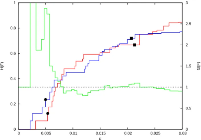
To analyze the information in the PI and RI maps, the standard procedure is to consider all possible forecasts to-gether. These are obtained by increasing F from 0 (corre-sponding to no hotspots on the map) to 1 (all active boxes on the map are identified as hotspots). The plot of H ver-sus F is the relative operating characteristic (ROC) diagram. Varying the threshold value for both the PI and RI fore-casts, we have obtained the values of H and F given in Fig. 5, blue for the PI forecasts and red for the RI fore-casts. The results corresponding to the maps given in Fig. 4 and the contingency tables given in Table 2 are given by the filled symbols. The forecast with 29 hotspot boxes (Fig. 5a and Table 2a) has FP I=0.00498, HP I=0.235 and
FRI=0.00537, HRI=0.125. The forecast with 127 hotspot
boxes (Fig. 5b and Table 2b) has FP I=0.0207, HP I=0.719
and FRI=0.0213, HRI=0.666. Also shown in Fig. 5 is a gain
curve (green) defined by the ratio of HP I(F ) to HRI(F ).
Gain values greater than unity indicate better performance using the PI map than using the RI map. The horizontal dashed line corresponds to zero gain. From Fig. 5 it can be seen that the PI approach outperforms (is above) the RI un-der many circumstances and both outperform a random map, where H =F , by a large margin.
10 Discussion
The fundamental question is whether forecasts of the time and location of future earthquakes can be accurately made. It is accepted that long term hazard maps of the expected rate of occurrence of earthquakes are reasonably accurate. But is it possible to do better? Are there precursory phenomena that will allow earthquakes to be forecast?
It is actually quite surprising that immediate local precur-sory phenomena are not seen. Prior to a volcanic eruption, increases in regional seismicity and surface movements are generally observed. For a fault system, the stress gradually increases until it reaches the frictional strength of the fault and a rupture is initiated. It is certainly reasonable to hy-pothesize that the stress increase would cause increases in background seismicity and aseismic slip. In order to test this hypothesis the Parkfield Earthquake Prediction Experi-ment was initiated in 1985. The expected Parkfield earth-quake occurred beneath the heavily instrumented region on 28 September 2004. No local precursory changes were ob-served (Lindh, 2005).
In the absence of local precursory signals, the next ques-tion is whether broader anomalies develop, and in particular whether there is anomalous seismic activity. It is this ques-tion that is addressed in this paper. Using a technique that has been successfully applied to the forecasting of El Ni˜no we have developed a systematic pattern informatics (PI) ap-proach to the identification of regions of anomalous seismic activity. Applications of this technique to California, Japan, and on a world-wide basis have successfully forecast the lo-cation of future earthquakes. It must be emphasized that this is not an earthquake prediction and does not state exactly
0 0.2 0.4 0.6 0.8 1 0 0.005 0.01 0.015 0.02 0.025 0.03 0 0.5 1 1.5 2 2.5 3 H(F) G(F) F
Fig. 5. Relative operating characteristic (ROC) diagram. Plot of hit
rates, H , versus false alarm rates, F , for the PI forecast (blue) and RI forecast (red). Also shown is the gain ratio (green) defined as
HP I(F )/HRI(F ). The filled symbols correspond to the threshold
values used in Fig. 4 and Table 2, solid circles for 29 hotspot boxes and solid squares for 127 hotspot boxes. The horizontal dashed line corresponds to zero gain.
when and where the next earthquake will occur. It is a fore-cast of where future earthquakes are expected to preferen-tially occur during a relatively long time window of ten years. The objective is to reduce the possible future sites of earth-quakes relative to a long term hazard assessment map.
Examination of the ROC diagrams indicates that the most important and useful of the suite of forecast maps are those with the least number of hotspot boxes, i.e. those with small values of the false alarm rate, F . A relatively high propor-tion of these hotspot boxes represent locapropor-tions of future large earthquakes, however these maps also have a larger number of failures-to-forecast. Exactly which forecast map(s) to be used will be a decision for policy-makers, who will be called upon to balance the need for few false alarms against the de-sire for the least number of failures-to-forecast.
Finally, we remark that the methods used to produce the forecast maps described here can be extended and improved. In it’s current state, the PI map is quite similar to the RI map. We have found modifications to the procedures described in Section 5 that allow the PI map to substantially outperform the RI map as indicated by the respective ROC diagrams. These methods are based on the approach of: 1) starting with the RI map and introducing improvements using the steps described for the PI method; and 2) introducing an additional averaging step. This new method is outlined in Appendix B, and a full analysis with results will be presented in a future publication.
Appendix A Explanation of the PI method
Here we summarize the current PI method as described by Rundle et al. (2003) and Tiampo et al. (2002b). The PI ap-proach is a six step process that creates a time-dependent
sys-tem state vector in a real valued Hilbert space and uses the phase angle to predict future states (Rundle et al., 2003). The method is based on the idea that the future time evolution of seismicity can be described by pure phase dynamics (Mori and Kuramoto, 1998; Rundle et al., 2000a,b). Hence, a real-valued seismic phase function ˆIi(tb, t )is constructed and
al-lowed to rotate in its Hilbert space. Since seismicity in active regions is a noisy function (Kanamori, 1981), only temporal averages of seismic activity are utilized in the method. The geographic area of interest is partitioned into N square bins with an edge length δx determined by the nature of the phys-ical system. For our analysis we chose δx=0.1◦≈11 km, corresponding to the linear size of a magnitude M ∼ 6 earth-quake. Later analysis showed that the method was sensitive to M∼5. Within each box, a time series Ni(t )is defined by
counting how many earthquakes with magnitude greater than Mminoccurred during the time period t to t +δt . Next, the ac-tivity rate function Ii(tb, T )is defined as the average rate of
occurrence of earthquakes in box i over the period tbto T :
Ii(tb, T ) =
PT
t =tbNi(t )
T − tb
. (A1)
If tb is held to be a fixed time, Ii(tb, T )can be interpreted
as the ith component of a general, time-dependent vector evolving in an N -dimensional space (Tiampo et al., 2002b). Furthermore, it can be shown that this N -dimensional cor-relation space is defined by the eigenvectors of an N × N correlation matrix (Rundle et al., 2000a,b). The activity rate function is then normalized by subtracting the spatial mean over all boxes and scaling to give a unit-norm:
ˆ Ii(tb, T ) = Ii(tb, T ) −N1 PNj =1Ij(tb, T ) q PN j =1[Ij(tb, T ) −N1 PNk=1Ik(tb, T )]2 . (A2)
The requirement that the rate functions have a constant norm helps remove random fluctuations from the system. Follow-ing the assumption of pure phase dynamics (Rundle et al., 2000a,b), the important changes in seismicity will be given by the change in the normalized activity rate function from the time period t1to t2:
1 ˆIi(tb, t1, t2) = ˆIi(tb, t2) − ˆIi(tb, t1). (A3)
This is simply a pure rotation of the N -dimensional unit vec-tor ˆIi(tb, T )through time. In order to both remove the last
free parameter in the system, the choice of base year, as well as to further reduce random noise components, changes in the normalized activity rate function are then averaged over all possible base-time periods:
1 ˆIi(t0, t1, t2) = Pt1
tb=t01 ˆIi(tb, t1, t2)
t1−t0 . (A4)
Finally, the probability of change of activity in a given box is deduced from the square of its base averaged, mean normal-ized change in activity rate:
In phase dynamical systems, probabilities are related to the square of the associated vector phase function (Mori and Ku-ramoto, 1998; Rundle et al., 2000b). This probability func-tion is often given relative to the background by subtracting off its spatial mean:
Pi0(t0, t1, t2) ⇒ Pi(t0, t1, t2) − 1 N N X j =1 Pj(t0, t1, t2), (A6)
Where P0 indicates the probability of change in activity is measured relative to the background.
Appendix B Updated method
1. The region of interest is divided into NB square boxes
with linear dimension 1x. Boxes are identified by a subscript i and are centered at xi. For each box, there is
a time series Ni(t ), which is the number of earthquakes
per unit time at time t larger than the lower cut-off mag-nitude Mc. The time series in box i is defined between
a base time tband the present time t .
2. All earthquakes in the immediate and eight surrounding regions of interest with magnitudes greater than a lower cutoff magnitude Mc are included. The lower cutoff
magnitude Mcis specified in order to ensure
complete-ness of the data through time, from an initial time t0to a final time t2. We use this extended, or Moore (1962), neighborhood to account for the uncertainty in event lo-cation and the arbitrary choice of where to center our boxes.
3. An intensity threshold is imposed such that only boxes that have historically been the most active are retained for analysis. The total number of earthquakes in each box from the initial time t0 to the final time t2 are counted, and boxes with counts less than the threshold are removed.
4. The seismic intensity in box i, Ii(tb, t ), between two
times tb<t, can then be defined as the average number
of earthquakes with magnitudes greater than Mcthat
oc-cur in the box per unit time during the specified time in-terval tbto t . Therefore, using discrete notation, we can
write: Ii(tb, t ) = 1 t − tb t X t0=t b Ni(t0), (B1)
where the sum is performed over increments of the time series, which can be days to years.
5. Three time intervals are considered: (a) A reference time interval from tbto t1.
(b) A second time interval from tb to t2, t2>t1. The change interval over which seismic activity changes
are determined is then t2−t1. The time tbis chosen
to lie between t0and t1. Typically we take t0=1932, t1=1990, and t2=2000. The objective is to quantify anomalous seismic activity in the change interval t1 to t2relative to the reference interval tbto t1. (c) The forecast time interval t2 to t3, for which the
forecast is valid.
6. Our measure of anomalous seismicity in box i is the difference between the seismic intensities at t1and t2: 1Ii(tb, t1, t2) = Ii(tb, t2) − Ii(tb, t1). (B2)
7. In order to compare the intensities from different time intervals, we require that they have the same statistical properties. We therefore normalize each of the seismic intensities both individually over all choices for tb and
aggregately at each choice for tb. This is performed by
subtracting the mean seismic activity and dividing by the standard deviation of the seismic activity. The sta-tistically normalized seismic intensity of box i is thus defined by 1 ˜Ii(tb, t1, t2) = 1Ii(tb, t1, t2)− < 1Ii(t1, t2) >T σT 1 ˆIi(tb, t1, t2) = 1 ˜Ii(tb, t1, t2)− < 1 ˜I (tb, t1, t2) >A σA , (B3) where <1Ii(t1, t2)>T is the mean intensity
differ-ence of box i averaged over all choices of tb,
<1 ˜I (tb, t1, t2)>A is the time averaged mean intensity
difference averaged over all the boxes at each choice of tb, and σT and σAare the respective standard deviations.
8. To reduce the relative importance of random fluctua-tions (noise) in seismic activity, we compute the aver-age change in intensity, 1Ii(t0, t1, t2)over many
differ-ent pairs of normalized intensity maps having the same change interval: 1Ii(t0, t1, t2) = 1 tmax−t0 tmax X tb=t0 q 1 ˆIi(tb, t1, t2)2, (B4)
where the sum is performed over increments of the time series for the distances between the normalized intensity differences and the background. In view of the fact that a time scale τ =t2−t1 has been implicitly chosen, the time tmaxis chosen to be tmax=t1−τ. This choice also gives the averaging time periods in the intervals tbto t1 and tb to t2more equal weight, thereby excluding the possibility of large fluctuations caused by main shocks occurring just prior to t1.
9. We hypothesize that the probability of a future earth-quake in box i, Pi(t0, t1, t2, ), is proportional to the square of the mean intensity change:
Pi(t0, t1, t2, ) ∝ 1Ii(t0, t1, t2)
2
The constant of proportionality can be determined by re-quiring unit probability but is not important to the anal-ysis.
10. To identify anomalous regions, we wish to compute the change in the probability Pi(t0, t1, t2, ) relative to the background so that we subtract the mean probability over all boxes. We denote this change in the probability by
1Pi(t0, t1, t2) = Pi(t0, t1, t2)− < Pi(t0, t1, t2) >A,(B6)
where <Pi(t0, t1, t2)>A is the background probability
for a large earthquake.
Hotspot pixels are defined to be the regions where 1Pi(t0, t1, t2)is positive. In these regions, Pi(t0, t1, t2)is
larger than the average value for all boxes (the background level). Note that since the intensities are squared in defin-ing probabilities, the hotspots may be due to either increases of seismic activity during the change time interval (activa-tion) or due to decreases (quiescence). We hypothesize that earthquakes with magnitudes larger than Mc+2 will occur
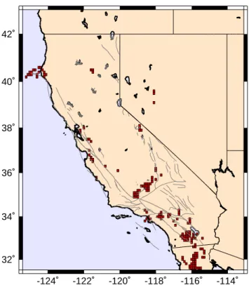
preferentially in hotspots during the forecast time interval t2 to t3. A forecast map for all of California and its surrounding area using this procedure is given in Fig. C1. More details and results will be presented in a future publication.
Appendix C Previous research
The PI method was first introduced by Rundle et al. (2002) as an implication of the diffusive mean-field nature of earth-quake dynamics. By treating seismicity as an example of a self-organizing threshold system they created forecast map for the occurrences of large earthquakes in southern Califor-nia. At this time the method was known as Phase Dynamical Probability Change (PDPC).
Tiampo et al. (2002b) defined the PDPC method in mathematical terms and provided a rational explanation for each step of the process. They also performed likelihood tests against various null hypothesis and showed the PDPC method forecasts earthquakes better than random catalogs and better than a simple measure of past seismicity.
Holliday et al. (2005a) later performed a systematic anal-ysis of the PDPC procedure. They varied the ordering of the steps and the parameter values and found optimal choices for the southern California region. The method at this time came to be know as Pattern Informatics (PI). Holliday et al. (2005b) then went on to investigate utilizing the PI method in a complex phase space. They determined that there is a small information gain for short-term (∼5 year) forecasts when us-ing complex eigenvectors rather than real-valued eigenvec-tors.
Nanjo et al. modified the PI method for use with the Japanese catalogs and successfully forecast the 23 October 2004 M=6.8 Niigata earthquake. Similarly, Chen and Holl-iday worked to modify the PI method for use with the Tai-wanese catalogs. Insights from this work have led to the
-124˚ -122˚ -120˚ -118˚ -116˚ -114˚ 32˚ 34˚ 36˚ 38˚ 40˚ 42˚
Fig. C1. Application of the modified PI method for all of California
and its surrounding area. Colored areas are the forecast hotspots for the occurrence of M≥5 earthquakes during the period 2005–2015.
modified method for California forecasting presented in Ap-pendix B and to a paper accepted for publication in Geophys-ical Review Letters (The 1999 Chi-Chi, Taiwan, earthquake as a typical example of seismic activation and quiescence).
Acknowledgements. This work has been supported by NASA Headquarters under the Earth System Science Fellowship Grant NGT5 (JRH), by a JSPS Research Fellowship (KZN), by an HSERC Discovery grant (KFT), by a grant from the US Depart-ment of Energy, Office of Basic Energy Sciences to the University of California, Davis DE-FG03-95ER14499 (JRH and JBR), and through additional funding from NSF grant ATM-0327558 (DLT) and the National Aeronautics and Space Administration under grants through the Jet Propulsion Laboratory to the University of California, Davis.
Edited by: G. Zoeller
Reviewed by: I. Zaliapin and another referee
References
Bakun, W. H. and Lindh, A. G.: The Parkfield, California, earth-quake prediction experiment, Science, 229, 619–624, 1985. Bowman, D. D. and King, G. C. P.: Accelerating seismicity and
stress accumulation before large earthquakes, Geophys. Res. Lett., 28, 4039–4042, 2001.
Bowman, D. D. and Sammis, C. G.: Intermittent criticality and the Gutenberg-Richter distribution, Pure Appl. Geophys, 161, 1945– 1956, 2004.
Bowman, D. D., Ouillon, G., Sammis, C. G., Sornette, A., and Sor-nette, D.: An Observational Test of the Critical Earthquake Con-cept, J. Geophys. Res., 103, 24 359–24 372, 1998.
Brehm, D. J. and Braile, L. W.: Intermediate-term earthquake pre-diction using precursory events in the New Madrid seismic zone, Bull. Seismol. Soc. Am., 88, 564–580, 1998.
Brehm, D. J. and Braile, L. W.: Intermediate-term Earthquake Pre-diction Using the Modified Time-to-failure Method in Southern California, Bull. Seismol. Soc. Am., 89, 275–293, 1999. Bufe, C. G. and Varnes, D. J.: Predictive modeling of the seismic
cycle of the greater San Francisco Bay region, J. Geophys. Res., 98, 9871–9883, 1993.
Bufe, C. G., Nishenko, S. P., and Varnes, D. J.: Seismicity trends and potential for large earthquakes in the Alaska-Aleutian region, Pure Appl. Geophys., 142, 83–99, 1994.
Chen, D., Cane, M. A., Kaplan, A., Zebian, S. E., and Huang, D.: Predictability of El Ni˜no in the past 148 years, Nature, 428, 733– 736, 2004.
Dobrovolsky, I. P., Zubkov, S. I., and Miachkin, V. I.: Estimation of the size of earthquake preparation zones, Pure Appl. Geophys., 117, 1025–1044, 1979.
Frankel, A. F.: Mapping seismic hazard in the central and eastern United States, Seismol. Res. Let., 60, 8–21, 1995.
Geller, R. J.: Earthquake prediction: A critical review, Geophys. J. Int., 131, 425–450, 1997.
Geller, R. J., Jackson, D. D., Kagen, Y. Y., and Mulargia, F.: Earth-quakes cannot be predicted, Science, 275, 1616–1617, 1997. Harte, D. and Vere-Jones, D.: The Entropy score and its uses in
earthquake forecasting, Pure Appl. Geophys., 162, 1229–1253, 2005.
Holliday, J. R., Rundle, J. B., Tiampo, K. F., Klein, W., and Don-nellan, A.: Systematic procedural and sensitivity analysis of the pattern informatics method for forecasting large (M ≥ 5) earth-quake events in southern California, Pure Appl. Geophys., in press, 2005a.
Holliday, J. R., Rundle, J. B., Tiampo, K. F., Klein, W., and Don-nellan, A.: Modification of the pattern informatics method for forecasting large earthquake events using complex eigenvectors, Tectonophysics, in press, 2005b.
Jaum´e, S. C. and Sykes, L. R.: Evolving towards a critical point: A review of accelerating seismic moment/energy release prior to large and great earthquakes, Pure Appl. Geophys., 155, 279–306, 1999.
Jolliffe, I. T. and Stephenson, D. B.: Forecast Verification, John Wiley, Chichester, 2003.
Kagan, Y. Y. and Jackson, D. D.: Probabilistic forecasting of earth-quakes, Geophys. J. Int., 143, 438–453, 2000.
Kanamori, H.: The nature of seismicity patterns before large earth-quakes, in Earthquake Prediction: An International Review, Geo-phys. Monogr. Ser., pp. 1–19, AGU, Washington, D. C., 1981. Kanamori, H.: Earthquake prediction: An overview, in International
Handbook of Earthquake & Engineering Seismology, edited by W. H. K. Lee, H. Kanamori, P. C. Jennings, and C. Kisslinger, pp. 1205–1216, Academic Press, Amsterdam, 2003.
Keilis-Borok, V.: Earthquake predictions: State-of-the-art and emerging possibilities, An. Rev. Earth Planet. Sci., 30, 1–33, 2002.
Keilis-Borok, V., Shebalin, P., Gabrielov, A., and Turcotte, D.: Re-verse tracing of short-term earthquake precursors, Phys. Earth Planet. Int., 145, 75–85, 2004.
Keilis-Borok, V. I.: The lithosphere of the earth as a nonlinear sys-tem with implications for earthquake prediction, Rev. Geophys.,
28, 19–34, 1990.
Keilis-Borok, V. I.: Intermediate-term earthquake prediction, Proc. Natl. Acad. Sci., 93, 3748–3755, 1996.
Keilis-Borok, V. I., Knopofff, L., and Rotvain, I. M.: Bursts of after-shocks, long-term precursors of strong earthquakes, Nature, 283, 259–263, 1980.
King, G. C. P. and Bowman, D. D.: The evolution of regional seis-micity between large earthquakes, J. Geophys. Res., 108, 2096– 2111, 2003.
Kossobokov, V. G., Keilis-Borok, V. I., Turcotte, D. L., and Mala-mud, B. D.: Implications of a statistical physics approach for earthquake hazard assessment and forecasting, Pure Appl. Geo-phys., 157, 2323–2349, 2000.
Lindh, A. G.: Success and failure at Parkfield, Seis. Res. Let., 76, 3–6, 2005.
Lomnitz, C.: Fundamentals of Earthquake Prediction, John Wiley, New York, 1994.
Main, I. G.: Applicability of time-to-failure analysis to acceler-ated strain before earthquakes and volcanic eruptions, Geophys. J. Int., 139, F1–F6, 1999.
Mason, I. B.: Binary Events, in Forecast Verification, edited by I. T. Joliffe and D. B. Stephenson, pp. 37–76, John Wiley, Chichester, 2003.
Mogi, K.: Earthquake Prediction, Academic Press, Tokyo, 1985. Molchan, G. M.: Earthquake predictions as a decision-making
problem, Pure Appl. Geophys., 149, 233–247, 1997.
Moore, E. F.: Machine models of self reproduction, in Proceedings of the Fourteenth Symposius on Applied Mathematics, pp. 17– 33, American Mathematical Society, 1962.
Mori, H. and Kuramoto, Y.: Dissipative Structures and Chaos, Springer-Verlag, Berlin, 1998.
Press, F. and Allen, C.: Patterns of seismic release in the southern California region, J. Geophys. Res., 100, 6421–6430, 1995. Prozoroff, A. G.: Variations of seismic activity related to locations
of strong earthquakes, Vychislitel’naya Seismologiya, 8, 71–72, 1975.
Robinson, R.: A test of the precursory accelerating moment release model on some recent New Zealand earthquakes, Geophys. J. Int., 140, 568–576, 2000.
Rundle, J. B., Klein, W., Gross, S. J., and Tiampo, K. F.: Dynamics of seismicity patterns in systems of earthquake faults, in Geo-complexity and the Physics of Earthquakes, edited by J. B. Run-dle, D. L. Turcotte, and W. Klein, vol. 120 of Geophys. Monogr. Ser., pp. 127–146, AGU, Washington, D. C., 2000a.
Rundle, J. B., Klein, W., Tiampo, K. F., and Gross, S. J.: Linear Pattern Dynamics in Nonlinear Threshold Systems, Phys. Rev. E., 61, 2418–2432, 2000b.
Rundle, J. B., Tiampo, K. F., Klein, W., and Martins, J. S. S.: Self-organization in leaky threshold systems: The influence of near-mean field dynamics and its implications for earthquakes, neuro-biology, and forecasting, Proc. Natl. Acad. Sci. USA, 99, 2514– 2521, Suppl. 1, 2002.
Rundle, J. B., Turcotte, D. L., Shcherbakov, R., Klein, W., and Sam-mis, C.: Statistical physics approach to understanding the multi-scale dynamics of earthquake fault systems, Rev. Geophys., 41, 1019–1038, 2003.
Sammis, C. G., Bowman, D. D., and King, G.: Anomalous seis-micity and accelerating moment release preceding the 2001-2002 earthquakes in northern Baha California, Mexico, Pure Appl. Geophys., 161, 2369–2378, 2004.
Scholz, C. H.: The Mechanics of Earthquakes & Faulting, Cam-bridg University Press, CamCam-bridge, 2nd edn., 2002.
Shebalin, P., Keilis-Borok, V., Zaliapin, I., Uyeda, S., Nagao, T., and Tsybin, N.: Advance short-term prediction of the large Tokachi-oki earthquake, September 25, M=8.1: A case history, Earth Planets Space, 56, 715–724, 2004.
Swets, J. A.: The relative operating characteristic in psychology, Science, 182, 990–1000, 1973.
Sykes, L. R. and Jaum´e, S. C.: Seismic activity on neighboring faults as a long-term precursor to large earthquakes in the San Francisco Bay area, Nature, 348, 595–599, 1990.
Sykes, L. R., Shaw, B. E., and Scholz, C. H.: Rethinking earthquake prediction, Pure Appl. Geophys., 155, 207–232, 1999.
Tiampo, K. F., Rundle, J. B., McGinnis, S., Gross, S. J., and Klein, W.: Eigenpatterns in southern California seismicity, J. Geophys. Res., 107, 2354, 2002a.
Tiampo, K. F., Rundle, J. B., McGinnis, S., and Klein, W.: Pat-tern dynamics and forecast methods in seismically active regions, Pure App. Geophys., 159, 2429–2467, 2002b.
Turcotte, D. L.: Earthquake prediction, An. Rev. Earth Planet. Sci., 19, 263–281, 1991.
Turcotte, D. L.: Fractals & Chaos in Geology & Geophysics, Cam-bridge University Press, CamCam-bridge, 2nd edn., 1997.
Utsu, T.: A list of deadly earthquakes in the world: 1500-2000, in International Handbook of Earthquake & Engineering Seismol-ogy, edited by W. H. K. Lee, H. Kanamori, P. C. Jennings, and C. Kisslinger, pp. 691–717, Academic Press, Amsterdam, 2003. Wyss, M.: Nomination of precursory seismic quiescence as a
sig-nificant precursor, Pure Appl. Geophys., 149, 79–114, 1997. Wyss, M. and Habermann, R. E.: Precursory seismic quiescence,
Pure Appl. Geophys., 126, 319–332, 1988.
Yang, W., Vere-Jones, D., and Li, M.: A proposed method for lo-cating the critical region of a future earthquake using the critical earthquake concept, J. Geophys. Res., 106, 4151–4128, 2001.


![Acidic Extracellular pH Promotes Activation of Integrin [alpha]v[beta]3](data:image/gif;base64,R0lGODlhAQABAIAAAP///wAAACH5BAEAAAAALAAAAAABAAEAAAICRAEAOw==)