HAL Id: hal-00319058
https://hal.archives-ouvertes.fr/hal-00319058
Submitted on 21 Nov 2006
HAL is a multi-disciplinary open access
archive for the deposit and dissemination of
sci-entific research documents, whether they are
pub-lished or not. The documents may come from
teaching and research institutions in France or
abroad, or from public or private research centers.
L’archive ouverte pluridisciplinaire HAL, est
destinée au dépôt et à la diffusion de documents
scientifiques de niveau recherche, publiés ou non,
émanant des établissements d’enseignement et de
recherche français ou étrangers, des laboratoires
publics ou privés.
R. M. Worthington
To cite this version:
R. M. Worthington. Diurnal variation of mountain waves. Annales Geophysicae, European
Geo-sciences Union, 2006, 24 (11), pp.2891-2900. �hal-00319058�
Ann. Geophys., 24, 2891–2900, 2006 www.ann-geophys.net/24/2891/2006/ © European Geosciences Union 2006
Annales
Geophysicae
Diurnal variation of mountain waves
R. M. Worthington
no affiliation
Received: 23 April 2006 – Revised: 9 October 2006 – Accepted: 19 October 2006 – Published: 21 November 2006
Abstract. Mountain waves could be modified as the
bound-ary layer varies between stable and convective. However case studies show mountain waves day and night, and above e.g. convective rolls with precipitation lines over mountains. VHF radar measurements of vertical wind (1990–2006) con-firm a seasonal variation of mountain-wave amplitude, yet there is little diurnal variation of amplitude. Mountain-wave azimuth shows possible diurnal variation compared to wind rotation across the boundary layer.
Keywords. Meteorology and atmospheric dynamics
(Con-vective processes; Turbulence; Waves and tides)
1 Introduction
Information on diurnal variation of mountain waves could be useful since the effect of, for instance, diurnal convection is uncertain. Convection could disrupt stable airflow of moun-tain waves (Ludlam, 1952), add to the mounmoun-tain peaks forc-ing waves (Wallforc-ington, 1977), or modify wave modes (Ralph et al., 1997) and amplitudes (Georgelin et al., 1996).
Mountain waves can modify downwind convection (Hosler et al., 1963; Booker, 1963; Starr and Browning, 1972; Winstead et al., 2002), however mountain-wave clouds can also occur above convection (Pigot and Hill, 1939; Sinha, 1966; M¨uller, 1983) covering the mountains, as if the wave source region could be higher than the mountain surface. Sea-breeze convection could also form an “additional effec-tive mountain” (Kozhevnikov et al., 1986).
Gravity waves above convection are usually categorised as convection waves, separate from mountain waves, and waves above orographic convection have also been inter-preted as a type of convection wave (Rovesti, 1970; Brad-bury, 1990; Hauf, 1993). However, waves above convective rolls over mountains (vertical wind tens of cm s−1or more,
on timescale of several hours, and disappearing with a turbu-lence layer for horizontal wind near zero) often appear typi-cal of mountain waves (Worthington, 2002).
Correspondence to: R.M. Worthington
(rmw092001@yahoo.com)
1.1 Definitions of mountain waves
Mountain waves could be defined as in standard theoretical models of wavelike air flow over a ridge, with the lowest streamlines usually following the mountain surface; similar waves modified by convection could be excluded from this category of classic or idealised mountain wave. Waves linked to orographic convection could have been wrongly identified as mountain waves in many studies using e.g. aircraft or radar data in the troposphere and stratosphere, without also mea-suring the boundary-layer structure.
However, terminology for waves above mountains is of-ten less specific about the cause of the waves, and instead based on wave characteristics, e.g. “standing wave” if re-maining almost static, or “orographic wave” if associated with mountains. A typical definition of mountain wave as “an atmospheric gravity wave, formed when stable air flow passes over a mountain or mountain barrier” (American Me-teorological Society, Glossary of Meteorology) does not ex-clude effects of convection, rotors and turbulence on moun-tain wave formation, or a wave launching height above the mountain surface (although “lee wave” could imply a moun-tain obstacle upwind, at the same height as the wave, and more directly causing the wave).
There are other variations on standard mountain-wave the-ory, such as a stagnant boundary layer absorbing waves in-stead of reflection at the ground (Smith et al., 2002; Jiang et al., 2006). Also there can be separate categories of moun-tain wave, such as “evening wave” (Roper and Scorer, 1952) for a mountain wave formed as convection stops and a stable boundary layer develops, maybe linked to katabatic wind.
This paper uses a definition of mountain wave as a stand-ing gravity wave above mountains (excludstand-ing e.g. propagat-ing gravity waves such as typical convection waves). The pa-per looks at mountain waves above convective rolls for two case studies in Sect. 2, since extensive convective rolls could be expected to disrupt daytime mountain waves, and provide an example of diurnal variation linked to stable–convective– residual boundary layer development above mountains (e.g., Kalthoff et al., 1998). Section 2.1 also includes weather radar measurements of precipitation lines for comparison with e.g. Kirshbaum and Durran (2005a). Section 3 then
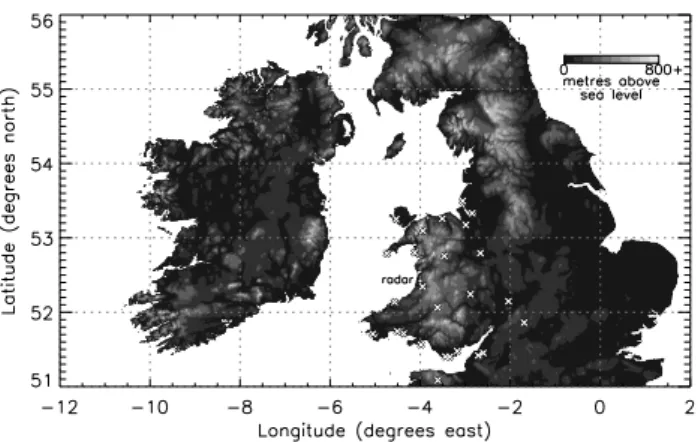
Fig. 1. Land height of the area for Figs. 2, 3, 5a, b, d–f, 6, 11.
×shows 26 surface weather sites for Figs. 8–10; “radar” is location of VHF and UHF radars for Figs. 4, 7–10, 12.
uses thousands of hours of VHF radar data to check for diur-nal and seasodiur-nal variations of mountain-wave amplitude, and Sect. 4 shows mountain-wave azimuth and compares VHF radar and satellite measurement methods.
2 Convective rolls, precipitation lines, and mountain waves
2.1 Case study, 1 October 2001
Miniscloux et al. (2001), Cosma et al. (2002) and Kirsh-baum and Durran (2005a) (“MCKD”) show weather radar measurements of along-wind precipitation lines above moun-tains. Numerical models imply these precipitation lines can be caused by convergence lines and convective rolls, trig-gered by mountains and mountain waves.
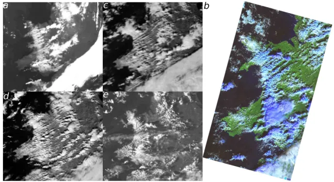
Figures 1–4 show a case study on 1 October 2001 with mountain waves above lines of convection and rain. Fig-ures 2a, c, d, e are from NOAA AVHRR (National Oceanic and Atmospheric Adminstration, Advanced Very High Res-olution Radiometer), and Fig. 2b from Landsat. There are cloud lines south-west to north-east, near parallel to the south-westerly surface wind, above mountains ∼52–53◦N, 3–4◦W.
Weather radar in Fig. 3 shows precipitation often also in lines, in the region of cloud lines above mountains in Fig. 2 (e.g. north and south of label “Birmingham”). Average rain distribution is similar to orographic rain increasing above high ground (e.g., Bonell and Sumner, 1992). Some south-west–north-east rain lines to the east at ∼12:00–15:00 UT advect with the wind instead of remaining above mountains, and orographic rain to north, ∼53–56◦N, 1–4◦W, is less lin-ear. There is also deeper convection in the cloud and rain lines, with thunder ∼11:00–12:00 UT at Birmingham, from a heavy rain area appearing near mountains of south Wales a few hours earlier. Occurrence of rain lines allows
compari-son with MCKD, using VHF radar to measure the wave field (e.g., R¨ottger, 2000), and with convective rain as another fac-tor in any diurnal effect of the convective boundary layer on mountain waves.
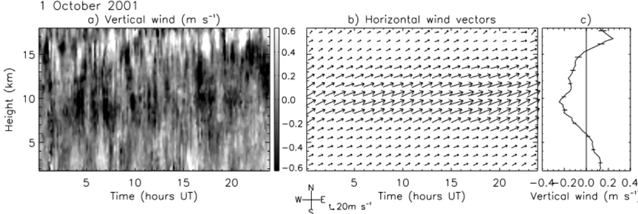
Figures 4a, c show bands of upward and downward ver-tical wind (W ) typical of mountain waves (e.g. Worthing-ton, 2002, Figs. 8a, 11a), measured using a 46.5 MHz VHF radar near Aberystwyth (Fig. 1). Figures 4a, c, 7a use a ver-tical radar beam; symmetric 6◦ beams show similar waves but are noisier above ∼16 km height. Vertical wavelength in-creases with jet wind speed as expected for mountain waves in Figs. 4a, b (e.g., Worthington et al., 2001). Therefore along-wind rain lines above mountains in Fig. 3 (MCKD) are occurring in a case study similar to other observations of mountain waves above convective rolls (Worthington, 2002, 2005).
Convective rolls could raise the effective surface of the mountains causing mountain waves, for sheared airflow over shallow convection (Sinha, 1966); alternatively vertical air motion in mountain waves could trigger convective rolls downwind within the lowest region of wave flow (Kirshbaum and Durran, 2005a,b). Mountain waves and convective rolls could be difficult to separate as cause and effect; whether mountain wave or convection starts further upwind could be significant. However cloud streets in Figs. 2b–d already start slightly upwind of the VHF radar measuring mountain waves in Fig. 4.
Figure 5 shows MODIS (Moderate-resolution Imaging Spectroradiometer) 250-m resolution images, with examples of wave cloud upwind of cloud streets near 62◦N, 7◦W (Fig. 5c); cloud streets possibly upwind of wave cloud then continuing over mountains higher than 1 km, 53◦N, 4◦W (Fig. 5f); and smooth cloud streets similar to lenticular wave cloud, 51.5◦N, 10◦W (Figs. 5a, b, d, e). In Figs. 5a, b, d, e
there also appear to be cloud streets above sea to south and west. Since convective rolls and mountain waves can often occur separately, or with either upwind, they could be de-scribed as separate processes which can coincide and inter-act, instead of one process causing the other.
For diurnal variation, Figs. 2–4 show mountain waves and also cloud and rain lines occur both night and day on 1 Oc-tober 2001, e.g. Fig. 2a at 02:26 UT. Sunrise and sunset are
∼06:15 and 17:55 UT. However along-wind cloud lines in Figs. 2a and 2b–e could be of different types such as streaks and rolls (e.g., Young et al., 2002; Shun et al., 2003). 2.2 Case study, 19 February 2004
Figure 6 shows cloud streets starting upwind, continuing above and downwind, of mountains. There are variations in thickness of the cloud streets, with appearance similar to “knots in strings”, above mountain areas of e.g. North York Moors (54.3◦N, 1◦W), Peak District (53◦N, 2◦W) and near Wales (52.5◦N, 3◦W) which are higher than e.g. Chiltern Hills in Tian et al. (2003). “Knot” spacing of ∼9 km is larger
R. M. Worthington: Diurnal variation of mountain waves 2893
Fig. 2. NOAA AVHRR images at (a) 02:26 UT, (c) 12:20 UT, (d) 14:01 UT, (e) 16:35 UT, and Landsat image at (b) 10:58 UT, 1 October 2001. (a) is infra-red channel 4, (b) false colour, and (c–e) visible channel 2, with image contrast and brightness adjusted. Locations in Figs. 2, 3, 5a, b, d–f, 6, 11 can be identified from coastline in Fig. 1.
Fig. 3. Sequence of weather radar images for 1 October 2001, at 1 h intervals, starting top left at 00:00 UT. Rows are 00:00–07:00 UT, 08:00–15:00 UT, 16:00–23:00 UT. Rain rate increases for blue, green, yellow, orange to red contours.
than individual cumulus clouds, not caused by satellite scan lines, and positions of “knots” are aligned perpendicular to the cloud streets, suggesting perhaps a wave pattern with phase lines perpendicular to cloud streets (Bradbury, 1990; Hindman et al., 2004).
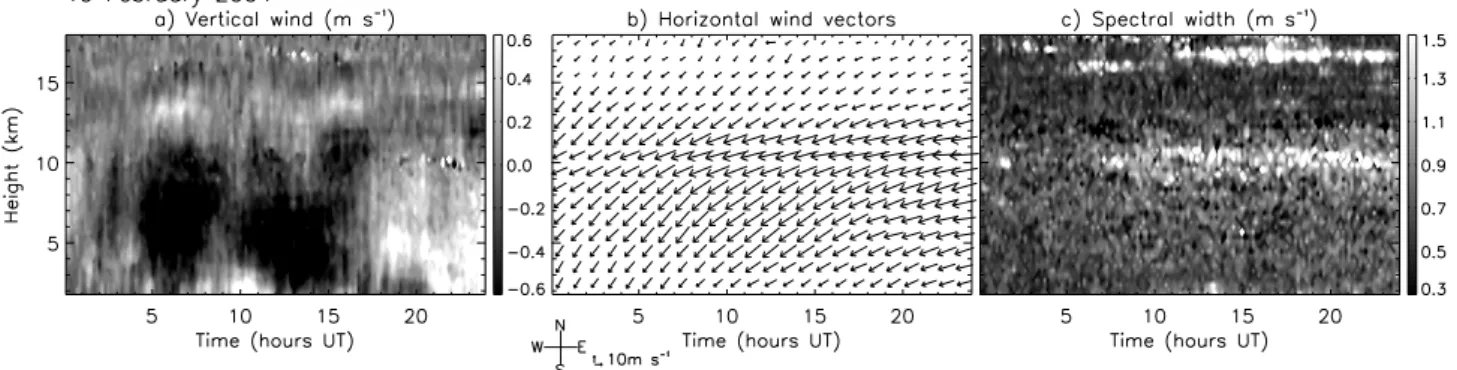
VHF radar, Fig. 7, shows mountain waves as in Worthing-ton (2002, Fig. 5). The cloud streets in Fig. 6 stop ∼8 km east, and restart ∼2 km west of the radar measuring Fig. 7, continuing for ∼10 km downwind over the sea. Mountain waves in Figs. 6, 7 are above, not only adjacent to cloud streets (Scorer, 1990). Also, there is possible orographic cirrus, 51–52◦N, 2–4◦W.
Vertical-beam spectral width corrected for beam-broadening (Fig. 7c) shows a turbulent layer for over 10 h at 16–17 km height, where mountain waves disappear at a critical layer (e.g., Worthington and Thomas, 1996). High spectral width near 10 km is partly spurious, caused by low signal-noise ratio below the tropopause at ∼11 km, and problems of exactly removing a substantial beam-broadening component in >30 m s−1horizontal wind. Since 16–17 km is above the regions of high jet-stream wind shear, Fig. 7 could show mountain-wave breaking not shear instability although horizontal wind speed is several m s−1.
Fig. 4. Height-time plots of (a) vertical wind and (b) horizontal wind vectors, measured by VHF radar, 52.4◦N, 4.0◦W; (c) time average of (a), 00:00–24:00 UT.
Fig. 5. MODIS images of south Ireland at (a) 11:35 UT, (b) 13:20 UT, 26 June 2004 and (d) 11:25 UT, (e) 13:10 UT, 22 June 2005; (c) Faroes at 13:10 UT, 18 August 2005; (f) Wales at 13:05 UT, 28 April 2005, showing onset of mixed convective rolls and mountain waves at coastlines. North is at the top, and surface wind is south to south-westerly for (a–f).
Typical convection waves should propagate downwind, whereas the waves above cloud streets in Fig. 7a keep the same phase for hours above the VHF radar. One explana-tion could be if mountain waves can exist through the con-vective boundary layer (Winstead et al., 2002), keeping the wave pattern “anchored” to the mountains; then waves as in Fig. 7a not only look like mountain waves, but can be partly caused as in standard mountain wave theory, modified by convection.
Satellite images at 02:35, 04:16 and 21:07 UT show wave cloud instead of the cloud streets in Fig. 6, yet Fig. 7 shows mountain waves and a turbulence layer for most of 19 Febru-ary 2004. Sunrise and sunset are at ∼07:25 and 17:35 UT. Sections 2.1 and 2.2 therefore show a lack of diurnal varia-tion of mountain waves, when variavaria-tion could be expected.
3 Diurnal and seasonal mountain-wave amplitude
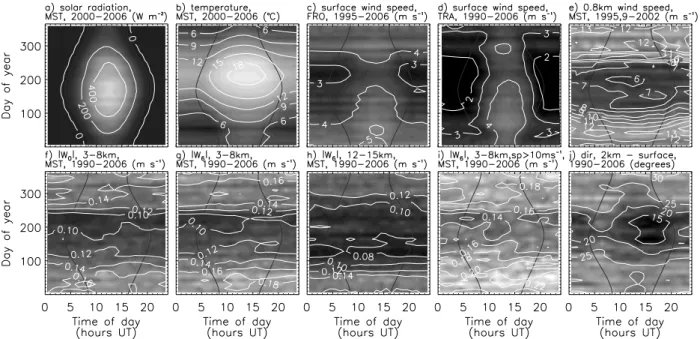
Figure 8 shows diurnal and seasonal variation of surface weather (Figs. 8a–d), and magnitude of vertical wind |W | (Figs. 8f–i) as a more direct measure of mountain-wave
R. M. Worthington: Diurnal variation of mountain waves 2895
Fig. 6. (a) NOAA AVHRR image at 14:10 UT, and (b) higher-resolution MODIS image at 13:20 UT, 19 February 2004. (a) is visible channel 2, (b) false colour.
Fig. 7. Height-time plots of (a) vertical wind, (b) horizontal wind vectors, (c) vertical-beam spectral width measured by VHF radar on 19 February 2004.
activity than wave clouds (e.g., Lester, 1978). Data sources are: 46.5 MHz VHF radar as in Figs. 4, 7, for >90 000 h, 1990–2006; co-located 915 MHz UHF radar, >19 000 h in February–March 1995 and November 1999–March 2002; co-located surface weather data, 2000–2006; and surface wind from ∼3 km west, 1995–2006, and ∼9 km south-south-east, 1990–2006. Figures 8a–e are for when VHF radar data also exist. VHF height resolution is 300 m, minimum height
∼1.7 km. Data for Fig. 8 are averaged to 1 h time resolu-tion, with similar results for e.g. 30 min or 10 min. Averaging of W measurements to 1 h resolution should remove typical convection waves (Kuettner et al., 1987; Gage et al., 1989; Sato, 1992; B¨ohme et al., 2004) with periods of tens of min-utes while retaining more static mountain waves.
Surface weather is included in Fig. 8 since if solar radia-tion, temperature and wind show minimal diurnal variation in winter at the VHF radar location, then diurnal variations of mountain waves might also be minimal. Sorting data for time of year shows also if any diurnal effect follows seasonal variation of sunrise and sunset time; Fig. 8 uses 30 inter-vals of ∼12.2 days. Figures 8a–d show some diurnal
vari-ation through winter. Surface wind differs in Figs. 8c and d, since Fig. 8c is measured near the top of a low hill, and Fig. 8d in a valley, more sheltered from prevailing wind, ex-cept for increased afternoon wind speed from e.g. sea breeze channelled in valleys, slope and valley winds, and convective boundary-layer mixing.
Wind speed higher in the boundary layer could be more correlated to mountain-wave amplitude than surface wind. Nastrom and Gage (1984) report |W | more correlated to 700 mB than 850 mB wind. Correlation of wind profiles is also possible to e.g. airglow (Sukhodoyev et al., 1989) or orographic rain (Neiman et al., 2002). Figure 9 shows correlation of wind profiles to |W | at 1.7–2.5 km height where mountain waves are immediately above their source region and below possible critical layers higher in the atmo-sphere. Correlation to |W | at e.g. 3–8 or 12–15 km instead of 1.7–2.5 km is more constant above ∼1 km. Correlation in Fig. 9 is only ∼0.35 or less, because of e.g. variations in hor-izontal position of mountain waves, and wave structure; also correlation profiles are altered by e.g. UHF data quality de-creasing with height, and the horizontal separation of VHF
Fig. 8. Diurnal and seasonal variation of (a) solar radiation, (b) temperature, (c–e) wind speed, (f–i) |W |, (j) wind rotation across the boundary layer, measured at: Aberystwyth Meso-Strato-Troposphere radar site (MST), marked on Fig. 1; ∼3 km west at Frongoch (FRO); and ∼9 km south-south-east at Trawscoed (TRA). (e) uses UHF radar; (j) uses VHF radar and average of surface wind sites in Fig. 1. Curved black lines show times of sunrise and sunset.
Fig. 9. Correlation of |W | at 1.7–2.5 km with: horizontal wind from radiosondes, VHF radar, UHF radar in 3 modes (green line: 192–193 m height resolution, February–March 1995 and Novem-ber 1999–March 2002; red line: 55 m, NovemNovem-ber 1999–May 2001; blue line: 96 m, May 2001–March 2002), and average of up to 26 surface sites in Fig. 1.
radar from radiosondes (typically tens of km; 50 km to their launch site at Aberporth). However, the height of maximum correlation is mostly ∼0.5–1 km, using all wind directions, or subsets as |W | increases with both westerly and easterly wind (Prichard et al., 1995). Figure 8e shows wind speed at 800 m height, with less diurnal variation, and faster wind speed in autumn and winter than Figs. 8c, d.
Figures 8f–i show diurnal and seasonal variation of |W | at 3–8 km measured using vertical radar beam (Fig. 8f) or sym-metric 6◦beams (Fig. 8g), and also at 12–15 km (Fig. 8h).
|W |increases in autumn and winter, similar to Fig. 8e and seasonal variation of mountain-wave clouds (Cruette, 1976; Lester, 1978). Diurnal variation of |W | is much less than seasonal variation and appears fairly random. Figure 8 can use subsets of wind speed, wind direction, and/or surface weather; Fig. 8i is for 2-km wind >10 m s−1, to check for diurnal variation in summer with faster wind speed. How-ever, there is a pattern similar to Figs. 8f–h for Fig. 8i, and also for: low-level wind from north-west-south 180◦ seg-ment mostly over the sea, or north-east-south 180◦segment over land (Fig. 1) with different surface heating and bound-ary layer; using e.g. maximum |W | at any height 3–8 km in-stead of mean; or using variance, W2. Also, W probability distribution is nearly constant with time of day.
Despite lack of diurnal variation in Figs. 8f–i, the bound-ary layer below mountain waves varies between stable and convective. However, even case studies in Figs. 4, 7 show lit-tle diurnal effect, above convective rolls. If mountain waves show almost no diurnal variation of amplitude, this could imply that mountain wave systems can have altered forcing mechanisms (stable and linear, or turbulent including con-vection) in the boundary layer without the wave field varying significantly above the boundary layer.
R. M. Worthington: Diurnal variation of mountain waves 2897
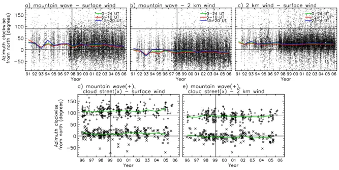
Fig. 10. Differences of wind and wave azimuths, using (a–c) VHF radar, 1991–2006, (d, e) satellites, 1996–2006, and surface wind averaged from up to 26 sites (Fig. 1). Green, red and blue lines show yearly medians, for 00:00–24:00 UT and other time intervals. Vertical lines in (a, b, d, e) show last data in Worthington (1999b, 2001). Dots in (c) are for every third data point. Mountain-wave azimuth is of horizontal wavevector for (a, b), and wave clouds for (d, e), measured clockwise from north.
4 Boundary-layer wind and wave azimuth
Another parameter to check for diurnal variation is azimuth of mountain-wave horizontal wavevector, on average be-tween the surface and tropospheric wind azimuths (Wor-thington, 1999b, 2001). Figures 10–12 are to check for di-urnal variation in over 15 years of data, and compare results from VHF radar and satellites, using an improved method of measuring wave azimuth on satellite images. Other mountain-wave parameters could also be useful, such as any diurnal variation of horizontal phase speed from zero, for e.g. numerical models.
Figure 10 shows mountain-wave azimuth measured as in Worthington (1999a,b, 2001), on average clockwise from surface wind in Figs. 10a, d, and anticlockwise from ∼2 km (1.7–2.3 km) wind in Figs. 10b, e. Wave azimuth from VHF radar uses height-time intervals 3–8 km ×1 h, with
|W |>0.05 m s−1 and azimuth error <20◦. Data to right of vertical lines in Figs. 10a, b, d, e are more recent than Wor-thington (1999b, 2001), to check that the wave and cloud azimuth results persist and do not disappear. Also Fig. 10c shows expected clockwise wind rotation with height in the boundary layer, to compare with Figs. 10a, b, d, e.
Liziola and Balsley (1997, 1998) use an alternative 3-radar method for measuring wave azimuth, which may give better results for propagating convection waves than for mountain waves (Carter et al., 1989).
Figures 10d, e use >500 satellite images (of >6500 visible-light images from the Universiy of Strasbourg
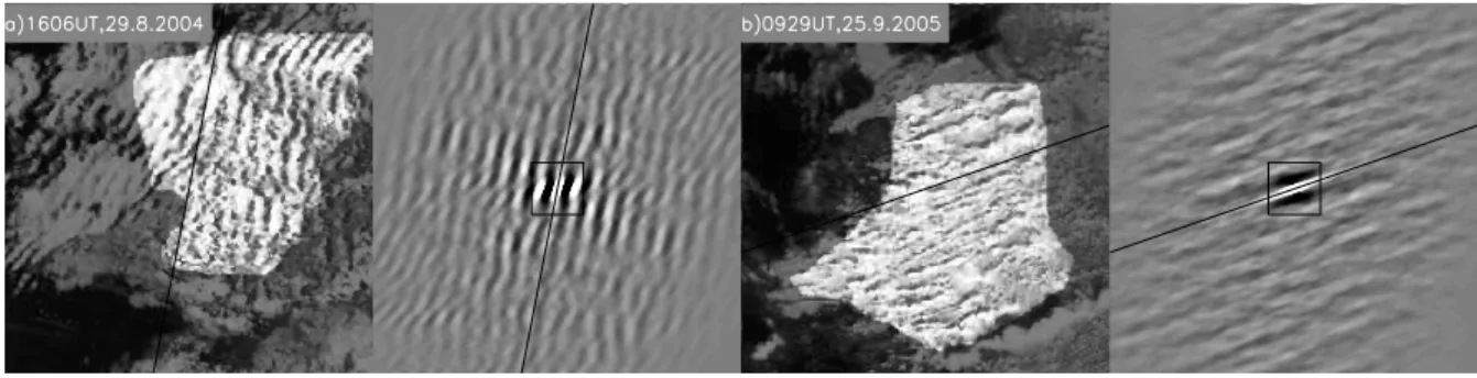
“quickFrance” archive, June 1996–March 2006). Instead of drawing lines by eye (e.g., Neumeister, 1971; Cruette, 1976; Worthington, 2001), cloud azimuths for ∼51.5–53.5◦N, 2– 5◦W are measured using 2-D autocorrelation; the processing method, modified from Mayor et al. (2003), is to
1. subtract a copy of each satellite image smoothed with
∼20 km running mean, to leave smaller-scale cloud fea-tures varying around approximately zero mean. 2. set all areas to zero except mountain-wave or
convective-roll cloud lines, above or near land since sur-face wind measurements in Fig. 1 are above land, also so mountain waves are above their source region, in-stead of being downwind lee waves.
3. take 2-D autocorrelation of each image using Fast Fourier Transform (and optionally subtract smoothed autocorrelation).
4. find the azimuth of the autocorrelation pattern, by ro-tating in steps of 1◦ using cubic interpolation, and averaging north-south in the square region of Fig. 11. The north-south average shows maximum east-west variations from its median, when the autocorrelation pattern is rotated with its lines north-south.
5. cloud azimuths (∼5%) are discarded if there are prob-lems from e.g. lines of cloud shadows, or multiple wave azimuths.
Fig. 11. Example satellite images of (a) mountain waves, (b) convective cloud streets, and autocorrelation of the unshaded areas of cloud. North is at the top. Diagonal lines show cloud azimuth from the region of autocorrelation marked by a square.
Fig. 12. Mountain-wave azimuths from VHF radar and satellite images, 1996–2006. Wave azimuth from satellite is perpendicular to cloud lines, pointing upwind. Time separation between radar and satellite data is 0, 1 or 2 h. The diagonal line is for equal radar and satellite azimuths.
Average surface wind for Figs. 10d, e is from up to 26 Met Office surface weather sites in Fig. 1, with time resolution 1 h and azimuth resolution 10◦(Aberdaron, Aberporth, Bris-tol Lulsgate, BrisBris-tol Weather Centre / Filton, Capel Curig, Cardiff Weather Centre, Crosby, Hawarden, Lake Vyrnwy, Liscombe, Little Rissington, Llanbedr, Milford Haven, Mumbles Head, Pembrey Sands, Pendine, Pershore, Rhoose, Rhyl, Sennybridge, Shawbury, Shobdon, Speke, St. Athan, Trawscoed, Valley). Averaging should also reduce sea breeze effects.
Figures 10d, e include cloud streets as in Worthington (2001), expected to be slightly clockwise from parallel to the surface wind, in checking if mountain-wave clouds are
slightly clockwise from perpendicular. There are more data before 1999 in Figs. 10d, e than Worthington (2001), since the autocorrelation method can also measure azimuth of patchy cloud lines. An average image rotation of 5◦ clock-wise from north is subtracted as in Worthington (2001).
Green, red and blue lines in Figs. 10a–c show yearly me-dians of the difference between wave and wind azimuth, for 00:00–24:00 UT and other time intervals. Red lines in Figs. 10a–c mostly show less positive or more negative az-imuth differences than blue lines. Horizontal wind rotation from surface to 2 km height is less for the daytime convective boundary layer (Fig. 8j), so red and blue lines in Fig. 10c are for 12:00–17:00 UT and 23:00–04:00 UT.
Plots similar to Fig. 8j for difference of mountain-wave and wind azimuth are more variable than Fig. 8j, but pos-sibly show wave azimuth is nearer to 2-km wind and fur-ther away from surface wind at e.g. 15:00–20:00 UT com-pared to 05:00–10:00 UT (blue, red lines in Figs. 10a, b). An explanation could be if, at the mountain-wave launching height (Shutts, 1997), the horizontal wavevector of mountain waves is on average parallel to horizontal wind (Worthing-ton, 1999b); in the afternoon, with a developed convective boundary layer, mountain wave azimuth could be parallel to upper-boundary-layer wind; in the morning, with more sta-ble residual-layer flow over a shallower convective bound-ary layer, mountain wave azimuth could instead be parallel to lower-boundary-layer wind, with much variability from profiles of e.g. wind shear and temperature lapse rate. Oc-currence of boundary-layer mountain-wave clouds at night, and convective clouds in daytime, could be consistent with a higher wave launching height instead of mountain waves ceasing in daytime.
Figure 12 compares measurements of mountain-wave az-imuth from VHF radar and satellite images. Mountain-wave cloud lines (Figs. 10d, e) are offset 90◦ from horizontal wavevector (Figs. 10a, b), so +90◦or –90◦is added to cloud line azimuth to obtain horizontal wavevector azimuth point-ing upwind; this allows scatterplot comparison over 0–360◦ azimuth of VHF radar (Figs. 10a, b), instead of 0–180◦ of cloud lines (Figs. 10d, e). Measurements are in the same
R. M. Worthington: Diurnal variation of mountain waves 2899
hour, or ±1, ±2 h to provide more data. VHF radar and satel-lite measurements of wave azimuth agree fairly well, with median difference <5◦ for Fig. 12, despite being limited to
occurrence of VHF aspect sensitivity and wave cloud.
5 Conclusions
Mountain waves near 52.4◦N, 4.0◦W show seasonal varia-tion of amplitude, but much less diurnal variavaria-tion despite the effects of boundary-layer convection. This negative result is however useful, in studying the effects of boundary layers on mountain waves.
Rain lines above mountains (Miniscloux et al., 2001; Cosma et al., 2002; Kirshbaum and Durran, 2005a,b) can oc-cur in convective rolls beneath typical mountain waves ob-served by VHF radar. Convective rolls can start upwind of mountain waves, not only triggered downwind.
Horizontal wavevector of mountain waves is between sur-face and tropospheric wind direction, both day and night, but possibly nearer to surface than 2-km wind azimuth in the morning, compared to evening.
Acknowledgements. NOAA AVHRR images are from University
of Strasbourg, NERC Satellite Receiving Station at Dundee Uni-versity, and Wokingham weather; MODIS from Rapid Response Project at NASA/GSFC; NASA/USGS Landsat image from ESA; weather radar from UK Met Office, BBC Weather and British Atmospheric Data Centre; NERC MST radar, and Met Office UHF radar and surface data from BADC; Met Office radioson-des from University of Wyoming and BADC; surface data also from NOAA Air Resources Laboratory and National Weather Ser-vice; autocorrelation program from http://cass185.ucsd.edu/help/ ssw/SSW frames.html and ETH Zurich; and land height data from GLOBE Project, NOAA NGDC.
Topical Editor U.-P. Hoppe thanks three referees for their help in evaluating this paper.
References
B¨ohme, T., Hauf, T., and Lehmann, V.: Investigation of short-period gravity waves with the Lindenberg 482 MHz tropospheric wind profiler, Q. J. R. Meteorol. Soc., 130, 2933–2952, 2004. Bonell, M. and Sumner, G.: Autumn and winter daily precipitation
areas in Wales, 1982–1983 to 1986–1987, Int. J. Climatol., 12, 77–102, 1992.
Booker, D. R.: Modification of convective storms by lee waves, Meteorol. Monogr., 5, 129–140, 1963.
Bradbury, T. A. M.: Links between convection and waves, Meteo-rol. Mag., 119, 112–120, 1990.
Carter, D. A., Balsley, B. B., Ecklund, W. L., Gage, K. S., Riddle, A. C., Garello, R., and Crochet, M.: Investigations of internal gravity waves using three vertically directed closely spaced wind profilers, J. Geophys. Res., 94, 8633–8642, 1989.
Cosma, S., Richard, E., and Miniscloux, F.: The role of small-scale orographic features in the spatial distribution of precipitation, Q. J. R. Meteorol. Soc., 128, 75–92, 2002.
Cruette, D.: Experimental study of mountain lee-waves by means of satellite photographs and aircraft measurements, Tellus, 28, 499–523, 1976.
Gage, K. S., Ecklund, W. L., and Carter, D. A.: Convection waves observed using a VHF wind-profiling Doppler radar during the Pre-Storm experiment, 24th Conf. Radar Meteorol., March 27– 31, 1989, Tallahassee, FL. (Amer. Meteorol. Soc., Boston, USA), 705–708, 1989.
Georgelin, M., Richard, E., and Petitdidier, M.: The impact of di-urnal cycle on a low-Froude number flow observed during the PYREX experiment, Mon. Weath. Rev., 124, 1119–1131, 1996. Hauf, T.: Aircraft observation of convection waves over southern
Germany – a case study, Mon. Weath. Rev., 121, 3282–3290, 1993.
Hindman, E. E., McAnelly, R. L., Cotton, W. R., Pattist, T., and Worthington, R. M.: An unusually high summertime wave flight, Technical Soaring, 28(4), 7–23, 2004.
Hosler, C. L., Davis, L. G., and Booker, D. R.: Modification of convective systems by terrain with local relief of several hundred meters, Zeitschr. Angew. Math. Phys., 14, 410–419, 1963. Jiang, Q., Doyle, J. D., and Smith, R. B.: Interaction between
trapped waves and boundary layers, J. Atmos. Sci., 63, 617–633, 2006.
Kalthoff, N., Binder, H.-J., Kossmann, M., V¨ogtlin, R., Corsmeier, U., Fiedler, F., and Schlager, H.: Temporal evolution and spa-tial variation of the boundary layer over complex terrain, Atmos. Env., 32, 1179–1194, 1998.
Kirshbaum, D. J. and Durran, D. R.: Observations and modeling of banded orographic convection, J. Atmos. Sci., 62, 1463–1479, 2005a.
Kirshbaum, D. J. and Durran, D. R.: Atmospheric factors governing banded orographic convection, J. Atmos. Sci., 62, 3758–3774, 2005b.
Kozhevnikov, V. N., Bibikova, T. N., and Zhurba, Y. V.: Oro-graphic waves, clouds and rotors with a horizontal axis above the Crimean Mountains, Izv. Atmos. Ocean. Phys., 22, 529–535, 1986.
Kuettner, J. P., Hildebrand, P. A., and Clark, T. L.: Convection waves: Observations of gravity wave systems over convectively active boundary layers, Q. J. R. Meteorol. Soc., 113, 445–467, 1987.
Lester, P. F.: A lee wave cloud climatology for Pincher Creek, Al-berta, Atmos.-Ocean, 16, 157–168, 1978.
Liziola, L. E. and Balsley, B. B.: Horizontally propagating quasi-sinusoidal tropospheric waves observed in the lee of the Andes, Geophys. Res. Lett., 24, 1075–1078, 1997.
Liziola, L. E. and Balsley, B. B.: Studies of quasi horizontally prop-agating gravity waves in the troposphere using the Piura ST wind profiler, J. Geophys. Res., 103, 8641–8650, 1998.
Ludlam, F. H.: Orographic cirrus clouds, Q. J. R. Meteorol. Soc., 78, 554–562, 1952 (and 79, 296–297, 1953).
Mayor, S. D., Tripoli, G. J., and Eloranta, E. W.: Evaluating large-eddy simulations using volume imaging lidar data, Mon. Weath. Rev., 131, 1428–1452, 2003.
Miniscloux, F., Creutin, J. D., and Anquetin, S.: Geostatistical anal-ysis of orogaphic rainbands, J. Appl. Meteorol., 40, 1835–1854, 2001.
M¨uller, D.: Leewellenbeobachtungen im Weserbergland – Einige Beispiele, Meteorol. Rundsch., 36, 166–168, 1983.
Nastrom, G. D. and Gage, K. S.: A brief climatology of vertical wind variability in the troposphere and stratosphere as seen by the Poker Flat, Alaska, MST radar, J. Clim. Appl. Meteorol., 23, 453–460, 1984.
Neiman, P. J., Ralph, F. M., White, A. B., Kingsmill, D. E., and Persson, P. O. G.: The statistical relationship between upslope flow and rainfall in California’s coastal mountains: Observations during CALJET, Mon. Weath. Rev., 130, 1468–1492, 2002. Neumeister, H.: Einige Untersuchungen ¨uber Zusammenh¨ange der
Charakteristika von Leewellen mit der Luftstr¨omung und der Temperaturschichtung in der Troposph¨are, Zeitschr. Meteorol., 22, 132–137, 1971.
Pigot, F. and Hill, R.: Notes on clouds observed from Glenn Cannel, Isle of Mull, Discovery, 2(new series), 60–62, 1939.
Prichard, I. T., Thomas, L., and Worthington, R. M.: The character-istics of mountain waves observed by radar near the west coast of Wales, Ann. Geophys., 13, 757–767, 1995,
http://www.ann-geophys.net/13/757/1995/.
Ralph, F. M., Neiman, P. J., Keller, T. L., Levinson, D. and Fe-dor, L.: Observations, simulations, and analysis of nonstationary trapped lee waves, J. Atmos. Sci., 54, 1308–1333, 1997. Roper, R. D. and Scorer, R. S.: Evening waves, Q. J. R. Meteorol.
Soc., 78, 415–419, 1952 (also, 79, 300–302, 1953).
R¨ottger, J.: ST radar observations of atmospheric waves over moun-tainous areas: a review, Ann. Geophys., 18, 750–765, 2000, http://www.ann-geophys.net/18/750/2000/.
Rovesti, P.: Thermal wave (‘thermo-onda’) soaring in Italy and Ar-gentina, OSTIV Publication XI, 1970.
Sato, K.: Vertical wind disturbances in the afternoon of mid-summer revealed by the MU radar, Geophys. Res. Lett., 19, 1943–1946, 1992.
Scorer, R. S.: Satellite as microscope (Sect. 12.2, Lee waves), Ellis Horwood Ltd., Chichester, 1990.
Shun, C. M., Lau, S. Y., and Lee, O. S. M.: Terminal Doppler weather radar observation of atmospheric flow over complex ter-rain during tropical cyclone passages, J. Appl. Meteorol., 42, 1697–1710, 2003.
Shutts, G.: Operational lee wave forecasting, Meteorol. Appl., 4, 23–35, 1997.
Sinha, M. C.: Mountain lee waves over Western Ghats, Indian J. Meteorol. Geophys., 17, 419–420, 1966.
Smith, R. B., Skubis, S., Doyle, J. D., Broad, A. S., Kiemle, C., and Volkert, H.: Mountain waves over Mont Blanc: Influence of a stagnant boundary layer, J. Atmos. Sci., 59, 2073–2092, 2002.
Starr, J. R. and Browning, K. A.: Observations of lee waves by high-power radar, Q. J. R. Meteorol. Soc., 98, 73–85, 1972. Sukhodoyev, V. A., Perminov, V. I., Reshetov, L. M., Shefov, N. N.,
Yarov, V. N., Smirnov, A. S., and Nesterova, T. N.: The oro-graphic effect in the upper atmosphere, Izv. Atmos. Ocean. Phys., 25, 681–685, 1989.
Tian, W., Parker, D. J., and Kilburn, C. A. D.: Observations and numerical simulation of atmospheric cellular convection over mesoscale topography, Mon. Weath. Rev., 131, 222–235, 2003. Wallington, C. E.: Meteorology for glider pilots, John Murray,
Lon-don, 3rd Edn., 1977.
Winstead, N. S., Sikora, T. D., Thompson, D. R., and Mourad, P. D.: Direct influence of gravity waves on surface-layer stress during a cold air outbreak, as shown by synthetic aperture radar, Mon. Weath. Rev., 130, 2764–2776, 2002.
Worthington, R. M.: Calculating the azimuth of mountain waves, using the effect of tilted fine-scale stable layers on VHF radar echoes, Ann. Geophys., 17, 257–272, 1999a.
Worthington, R. M.: Alignment of mountain wave patterns above Wales: A VHF radar study during 1990–1998, J. Geophys. Res., 104, 9199–9212, 1999b.
Worthington, R. M.: Alignment of mountain lee waves viewed us-ing NOAA AVHRR imagery, MST radar, and SAR, Int. J. Re-mote Sensing, 22, 1361–1374, 2001.
Worthington, R. M.: Mountain waves launched by convective activ-ity within the boundary layer above mountains, Boundary-Layer Meteorol., 103, 469–491, 2002.
Worthington, R. M.: Convective mountain waves above Cross Fell, northern England, Weather, 60, 43–44, 2005.
Worthington, R. M. and Thomas, L.: Radar measurements of critical-layer absorption in mountain waves, Q. J. R. Meteorol. Soc., 122, 1263–1282, 1996.
Worthington, R. M., Muschinski, A., and Balsley, B. B.: Bias in mean vertical wind measured by VHF radars: significance of radar location relative to mountains, J. Atmos. Sci., 58, 707–723, 2001.
Young, G. S., Kristovich, D. A. R., Hjelmfelt, M. R., and Foster, R. C.: Rolls, streets, waves, and more. A review of quasi-two-dimensional structures in the atmospheric boundary layer, Bull. Amer. Meteorol. Soc., 83, ES54–ES69, 2002.