HAL Id: hal-00703804
https://hal.archives-ouvertes.fr/hal-00703804
Submitted on 4 Jun 2012
HAL is a multi-disciplinary open access
archive for the deposit and dissemination of
sci-entific research documents, whether they are
pub-lished or not. The documents may come from
teaching and research institutions in France or
abroad, or from public or private research centers.
L’archive ouverte pluridisciplinaire HAL, est
destinée au dépôt et à la diffusion de documents
scientifiques de niveau recherche, publiés ou non,
émanant des établissements d’enseignement et de
recherche français ou étrangers, des laboratoires
publics ou privés.
in relation to environmental and biogeochemical
parameters during the late stages of the 2005 North
East Atlantic Spring Bloom
Karine Leblanc, C. E. Hare, Y. Feng, G. M. Berg, G. R. Ditullio, A. Neeley, I.
Benner, C. Sprengel, A. Beck, S. A. Sanudo-Wilhelmy, et al.
To cite this version:
Karine Leblanc, C. E. Hare, Y. Feng, G. M. Berg, G. R. Ditullio, et al.. Distribution of calcifying and
silicifying phytoplankton in relation to environmental and biogeochemical parameters during the late
stages of the 2005 North East Atlantic Spring Bloom. Biogeosciences, European Geosciences Union,
2009, 6, pp.2155-2179. �hal-00703804�
www.biogeosciences.net/6/1/2009/
© Author(s) 2009. This work is distributed under the Creative Commons Attribution 3.0 License.
Biogeosciences
Distribution of calcifying and silicifying phytoplankton in relation to
environmental and biogeochemical parameters during the late
stages of the 2005 North East Atlantic Spring Bloom
K. Leblanc1, C. E. Hare2, Y. Feng3, G. M. Berg4, G. R. DiTullio5, A. Neeley6, I. Benner7,8, C. Sprengel7, A. Beck9, S. A. Sanudo-Wilhelmy10, U. Passow7,12, K. Klinck7, J. M. Rowe11, S. W. Wilhelm13, C. W. Brown14, and
D. A. Hutchins10
1Universit´e d’Aix-Marseille; CNRS; LOPB-UMR 6535, Laboratoire d’Oc´eanographie Physique et Biog´eochimique;
OSU/Centre d’Oc´eanologie de Marseille, UMR 6535, Campus de Luminy Case 901, 163 Avenue de Luminy, 13288 Marseille Cedex 09, France
2Woods Hole Group, Inc., 100 Carlson Way, Suite 9, Dover, Delaware, 19901, USA
3Laboratory of Marine Ecology and Environmental Science, Institute of Oceanology, Chinese Academy of Sciences,
Qingdao 266071, China
4Department of Environmental Earth System Science, Stanford University, Stanford, CA 94305, USA 5Hollings Marine Laboratory, College of Charleston, Charleston, SC 29412, USA
6NASA/SSAI/BWTech 1450 S Rolling Road Halethorpe, MD 21227, USA
7Alfred Wegener Institute for Polar and Marine Research, Am Handelshafen 12, 27570 Bremerhaven, Germany 8Romberg Tiburon Center for Environmental Studies San Francisco State University 3152 Paradise Drive Tiburon,
CA 94920, USA
9Max-Planck-Institute for Marine Microbiology, Celsiusstrasse 1, 28359 Bremen, Germany
10Department of Biological Sciences, University of Southern California, 3616 Trousdale Parkway, Los Angeles,
CA 90089, USA
11University of Nebraska, the Department of Biological Sciences, in Lincoln, NE 68583, USA 12Marine Science Institute, University California Santa Barbara, CA 93106, USA
13Department of Microbiology, University of Tennessee, Knoxville, TN 37996, USA
14Center for Satellite Applications and Research, National Oceanographic and Atmospheric Administration,
College Park, MD 20740, USA
Received: 31 May 2009 – Published in Biogeosciences Discuss.: 19 June 2009 Revised: 23 September 2009 – Accepted: 24 September 2009 – Published:
Abstract. The late stage of the North East Atlantic (NEA) spring bloom was investigated during June 2005 along a transect section from 45 to 66◦N between 15 and 20◦W in order to characterize the contribution of siliceous and cal-careous phytoplankton groups and describe their distribution in relation to environmental factors. We measured several biogeochemical parameters such as nutrients, surface trace metals, algal pigments, biogenic silica (BSi), particulate in-organic carbon (PIC) or calcium carbonate, particulate or-ganic carbon, nitrogen and phosphorus (POC, PON and POP, respectively), as well as transparent exopolymer particles
Correspondence to: K. Leblanc
(TEP). Results were compared with other studies undertaken in this area since the JGOFS NABE program. Characteris-tics of the spring bloom generally agreed well with the ac-cepted scenario for the development of the autotrophic com-munity. The NEA seasonal diatom bloom was in the late stages when we sampled the area and diatoms were con-strained to the northern part of our transect, over the Ice-landic Basin (IB) and IceIce-landic Shelf (IS). Coccolithophores dominated the phytoplankton community, with a large distri-bution over the Rockall-Hatton Plateau (RHP) and IB. The Porcupine Abyssal Plain (PAP) region at the southern end of our transect was the region with the lowest biomass, as demonstrated by very low Chla concentrations and a com-munity dominated by picophytoplankton. Early depletion
of dissolved silicic acid (DSi) and increased stratification of the surface layer most likely triggered the end of the diatom bloom, leading to coccolithophore dominance. The chronic Si deficiency observed in the NEA could be linked to mod-erate Fe limitation, which increases the efficiency of the Si pump. TEP closely mirrored the distribution of both biogenic silica at depth and prymnesiophytes in the surface layer sug-gesting the sedimentation of the diatom bloom in the form of aggregates, but the relative contribution of diatoms and coc-colithophores to carbon export in this area still needs to be resolved.
1 Introduction
The North Atlantic is an important seasonal sink for atmo-spheric CO2through intense convection of cold surface
wa-ters and elevated primary productivity during spring (Watson et al., 1991). It also appears to be a large sink for anthro-pogenic CO2 (Gruber, 1996). The NABE (North Atlantic
spring Bloom Experiment) program (1989 and 1990) showed that CO2variability was strongly related to the
phytoplank-ton bloom dynamics (Ducklow and Harris, 1993).
The spring bloom starts to develop following surface warming and stratification in March–April, and benefits from the large nutrient stocks available following the intense win-ter convective mixing of surface wawin-ters. It propagates north-ward as surface stratification progresses in what has been described as a rolling green patchwork, strongly riddled by mesoscale and eddy activity (Robinson et al., 1993). A pro-posed mechanism for the spring bloom in the North East At-lantic (NEA) involves a rapid diatom growth and dominance in the early spring, followed by a more diverse community of prymnesiophytes, cyanobacteria, dinoflagellates and green algae later in the season (Sieracki et al., 1993).
At high latitudes, the NEA is also the site of one of the largest coccolithophore blooms observed anywhere in the ocean. Satellite imagery annually reveals extensive coccol-ithophore blooms in surface waters between 50 and 63◦N as well as on the Icelandic shelf (Holligan et al., 1993; Brown and Yoder, 1994; Balch et al., 1996; Iglesias-Rodriguez et al., 2002). It has been hypothesized that the coccolithophore bloom frequently follows the diatom bloom as the growing season progresses. Progressively more stratified surface wa-ters receive stronger irradiances with correspondingly more severe nutrient limitation. Coccolithophores have lower half-saturation constants for dissolved inorganic nitrogen (DIN) and phosphorus (DIP) compared to diatoms (Eppley et al., 1969; Iglesias-Rodriguez et al., 2002), and their ability to uti-lize a wide variety of organic nitrogen or phosphorus sources (Benner and Passow, 2009) has been invoked as major factors leading to this succession in surface waters.
Dissolved silicic acid (DSi) availability is also thought to play a major role in phytoplankton community succession.
Recurrent DSi depletion has been observed in the NEA dur-ing the NABE (1989) and POMME (2001) programs (Lochte et al., 1993; Sieracki et al., 1993; Leblanc et al., 2005). In these studies during the phytoplankton bloom, DIN stocks were still plentiful while DSi was almost depleted due to diatom uptake in early spring. Thus, the stoichiometry of initially available nutrients following winter deep mixing likely plays a crucial role in the structural development of the spring bloom, which feeds back on the availability of nu-trients in the mixed layer (Moutin and Raimbault, 2002).
The partitioning of primary production between calcifiers and silicifiers is of major importance for the efficiency of the biological pump. Both CaCO3and SiO2act as ballast
min-erals, but their differential impact on C fluxes to depth is still a matter of debate (Boyd and Trull, 2007). The efficiency of the biological pump is also largely a matter of packag-ing of sinkpackag-ing material, e.g. in faecal pellets or as aggre-gates with varying transparent exopolymer particles (TEP) contents. TEP are less dense than seawater and consequently higher concentrations of TEP result in decreased sinking ve-locities (Passow, 2004).
The objectives of the NASB 2005 (North Atlantic Spring Bloom) program was to describe the phytoplankton blooms in the NEA during June 2005 and identify the relative con-tribution of the two main phytoplankton groups producing biominerals, namely diatoms and coccolithophores, which are thought to play a major role in carbon export to depth. Their distribution in the mixed layer and the strong latitudi-nal gradients observed along the 20◦W meridian from the Azores to Iceland are discussed in relation to nutrient and light availability as well as water column stratification.
Our results are compared and contrasted with previ-ous studies carried out in this sector [BIOTRANS 1988 (Williams and Claustre, 1991), NABE 1989 (Ducklow and Harris, 1993), PRIME 1996 (Savidge and Williams, 2001), POMME 2001 (M´emery et al., 2005), AMT (Aiken and Bale, 2000)] and we discuss whether a clear scenario for the NEA spring/summer bloom can be proposed. Our data set is used to ask several key questions about this biogeochemically crit-ical part of the ocean: are the coccolithophore blooms of-ten indicated by the large calcite patches seen in satellite images a major component of the phytoplankton bloom in the NEA? Which environmental factors can best explain the relative dominance of coccolithophores vs. diatoms in this high latitude environment? What causes recurrent silicic acid depletion in the NEA and what are the potential conse-quences for phytoplankton composition and carbon export? We addressed these questions by investigating the distribu-tion of the major biogeochemical parameters such as partic-ulate opal, calcite, algal pigments, particpartic-ulate organic car-bon (POC), nitrogen (PON) and phosphorus (POP) as well as TEP concentrations in relation to environmental factors such as light, nutrients and trace metals along a transect near the 20◦W meridian between the Azores and Iceland.
2 Material and methods 2.1 Study area
The NASB 2005 (North Atlantic Spring Bloom) transect was conducted on the R/V Seaward Johnson II in the NEA Ocean between 6 June and 3 July 2005. The cruise track was lo-cated between 15◦W and 25◦W, starting at 45◦N north of the Azores Islands and ending at 66.5◦N west of Iceland (Fig. 1a). The South-North transect was initially intended to track the 20◦W meridian but included several deviations in order to follow real-time satellite information locating ma-jor coccolithophore blooms and calcite patches. Ship-board CO2, temperature and nutrient perturbation experiments
ac-companied the field measurements presented here (compan-ion papers: Feng et al., 2009; Rose et al., 2009; Lee et al., 2009; Benner et al., 2009).
2.2 Sample collection and analysis 2.2.1 Hydrographic data
CTD casts from the surface to 200 m depths were performed at 37 stations along the transect to emphasize biogeochem-ical processes in the surface layer. Physbiogeochem-ical characteristics of the surface water will be included in a description of the main water masses present in the area. Surface water can greatly influence biological processes and their characteris-tics help determine the location of fronts, eddies, vertical stratification and hydrological provinces that were crossed. Water samples were collected using 10 L Niskin bottles on a rosette, mounted with a Seabird 9+ CTD equipped with pho-tosynthetically active radiation (PAR), fluorescence and oxy-gen detectors. Surface trace metal samples were collected using a surface towed pumped “fish” system (Hutchins et al., 1998). Topographical information and section plots were ob-tained using ODV software (Schlitzer, R., Ocean Data View, http://odv.awi.de, 2007). The depths of the mixed layer (Zm) and the nutricline (Zn) were determined as the depth of the strongest gradient in density and dissolved inorganic nitro-gen (DIN) respectively between two measurements between the surface and 200 m. Treated CTD density data averaged every 0.5 m were used for the calculation of Zm, while nutri-ent data collected at 12 depths on average with Niskin bot-tles were used to compute Znover the 0–200 m layer. At the highest concentration gradient identified between to Niskin measurements, Znwas determined as the depth of the upper bottle. The euphotic depth (Ze) was calculated as the 1% light level using CTD PAR data averaged every 0.5 m. 2.2.2 Dissolved nutrients and trace metals
Concentrations of DIN (nitrate+nitrite), DIP and DSi were determined colorimetrically on whole water samples by stan-dard autoanalyzer techniques (Futura continuous flow ana-lyzer, Alliance Instruments) as soon as the samples were
col-lected at each station. Near-surface water samples (∼10 m depth) for trace metal analysis were collected with a pump system using an all-Teflon diaphragm pump (Bruiser) and PFA Teflon tubing attached to a weighted PVC fish (Hutchins et al., 1998). The tubing was deployed from a boom off the side of the ship outside of the wake, and samples were collected as the ship moved forward into clean water at approximately 5 knots. After flushing the tubing well, a 50 L polyethylene carboy was filled in a clean van and used for subsampling under HEPA-filtered air (removing particles above 0.3 µm diameter). All sampling equipment was exhaustively acid-washed, and trace-metal clean han-dling techniques were adhered to throughout (Bruland et al., 1979). One-liter samples were filtered though 0.22 µm pore size polypropylene Calyx capsule filters into low-density polyethylene bottles, and acidified to pH<2 with ultrapure HCl after conclusion of the cruise. Dissolved metals were preconcentrated from 250 mL seawater using APDC/DDDC organic solvent extraction (Bruland et al., 1979). Chloroform extracts were brought to dryness, oxidized with multiple aliquots of concentrated ultrapure HNO3, dried again, and
reconstituted with 2 mL of 1N ultrapure HNO3. Samples for
particulate and intracellular metals were collected onto 2 µm polycarbonate filter membranes held in polypropylene filter sandwiches. For intracellular metals determination, cells re-tained by the filters were washed with 5 mL of an oxalate solution to remove surface-adsorbed metals (Tovar-Sanchez et al., 2003), and rinsed with filtered, Chelex-cleaned seawa-ter (Tang and Morel, 2006). Maseawa-terial on the total and intra-cellular particulate filters was digested at room temperature with 2 mL ultrapure aqua regia and 50 µL HF. Concentrated acids were evaporated to near dryness and reconstituted with 2 mL of 1N ultrapure HNO3. Dissolved and particulate metal
extracts were analyzed by direct injection ICP-MS (Ther-moFisher Element2) following 10-fold dilution, with indium as an internal standard.
2.2.3 Particulate matter
PIC, POC and PON: water samples (400 mL) were filtered onto precombusted glass fibre filters (Whatman GF/F) and dried at 50◦C. At the laboratory, filters were HCl fumed for 4 h in a desiccator, redried in an oven at 60◦C (Lorrain et al., 2003) and measured on a Carlo Erba Strumentazione Nitro-gen Analyzer 1500 to determine POC and PON concentra-tions. A duplicate of each sample was run directly without fuming to obtain Total Particulate Carbon (TPC). PIC con-centrations were calculated from the difference between TPC and POC.
POP: between 750 mL and 1 L samples were filtered onto precombusted glass fibre filters (Whatman GF/F) and rinsed with 2 mL of 0.17 M Na2SO4. The filters were then placed
in 20 mL precombusted borosilicate scintillation vials with 2 mL of 17 mM MnSO4. The vials were covered with
Figure 1 32 34 11 14 16 18 20 27 2122 24 2 5 7 9 1 3 4 6 8 10 12 13 15 17 19 26 28 23 25 29 30 31 33 35 36 37 2 NAW MNAW ? ? NAC NAC CSC NIIC IC PW EGC FC Mid -Atl anti c R idge Iceland Basin Rockall-Hatton Plateau Porcupine Abyssal Plain Bay of Biscay Azo re s-Bis cay Ris e Mid -Atl an tic Rid ge Iberian Abyssal Plain 3000 5000 2500 2000 George Bligh Bank W yville -Thom pson Ridge 24 34 32 27 22 21 20 18 16 14 11 9 7 5 A C PW 37 1 - 5 6 - 33 36 35 MNAW NAW PAP RPH IB IS B Porcupine Abyssal Plain Rockall Hatton Plateau Iceland Basin Icelandic Shelf 1000 2000 3000 4000 5000 45 50 55 60 65 Latitude [°N] D e p th [ m ] D e p th [ m ] 33.5 34 34.5 35 35.5 Salinity [PSU] 36 T e m p e ra tu re [ °C ] 5 10 15 D e p th [ m ] 0 50 100 150 200
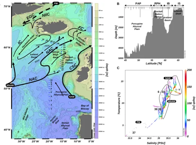
Fig. 1. (A) Map of the study area with stations sampled and main currents theoretical position according to literature. NAW: North Atlantic Waters; MNAW: Modified North Atlantic Waters; NAC: North Atlantic Current; CSC: Continental Slope Current; NIIC: North Icelandic Irminger Current; IC: Irminger Current; EGC: East Greenland Current; FC: Faroe Current. (B) Transect topography plotted using ODV, and depth of the CTDs along the transect. (C) T-S diagram of the water masses between 0 and 200 m for the 37 stations sampled.
analysis. The vials were combusted at 450◦C for 2 h, and after cooling 5 mL of 0.2 N HCl were added to each vial for final analysis. Vials were tightly capped and heated at 80◦C for 30 min to digest POP into inorganic phosphorus. The di-gested POP samples were analyzed with the standard molyb-date colorimetric method (Solorzano and Sharp, 1980).
BSi (Biogenic Silica): samples for biogenic silica mea-surements (1 L) were filtered onto polycarbonate filters (0.6 µm, 47 mm) and stored in plastic Petri dishes. Filters were dried at 60◦C for 24 h and then stored at room temper-ature. Samples were analyzed for biogenic silica following the digestion of silica in hot 0.2 N NaOH for 45 min (Nelson et al., 1989).
TEP: between 150 mL (surface) and 400 mL (at depth) samples were filtered onto 0.4 µm polycarbonate filters and directly stained with Alcian blue. Three replicates per depth and six replicate blanks per day were prepared. Stained fil-ters were frozen until analysis or analyzed directly according to Passow and Alldredge (1995). Briefly, filters were soaked in 6 mL 80% H2SO4. After 2 to 8 h the absorption of the
re-sulting solution was measured colorimetrically at 787 nm in a 1 cm cuvette. Gum Xanthan was used for calibration, thus
this method compares the staining capability of TEP to that of Gum Xanthan and values are expressed as Gum Xanthan equivalent per L (µg Xeq L−1).
2.2.4 Taxonomic information
Pigments: water samples (1 L) were filtered onto glass fibre filters (Whatman GF/F) and stored in liquid nitrogen until analysis. Samples were analyzed on an Agilent 1100 HPLC (High Performance Liquid Chromatography) system with diode array and fluorescence detection. Elution gradients and protocols were described in detail elsewhere (DiTullio and Geesey, 2002).
Coccolithophore cell counts: water samples of 400 mL were filtered onto cellulose nitrate filters (0.45 µm, 47 mm) and dried at 50◦C for coccolithophore cell counts. Pieces of the filters were sputter-coated with gold-palladium and im-aged with a Philips XL-30 digital scanning field-emission electron microscope (SEM). Coccolithophores were counted from SEM images and coccolithophores L−1were calculated from counts, counting area, filter area and filtered volume. Coccolithophores were only counted at selected depths at
sites of elevated PIC concentrations (St. 10, 12, 19, 23, 29, 31, 33, 34).
2.2.5 Satellite images
Monthly satellite MODIS Chla and calcite composite im-ages were obtained from the Level 3 browser available on the NASA Ocean Biology Processing Group website (http: //oceancolor.gsfc.nasa.gov/).
2.2.6 Statistical correlation analyses
A non-parametric two-tailed Spearman Rank correlation co-efficient was used as a measure of correlation between the main biogeochemical parameters as the criterion of normal distribution was not met for any of them.
3 Results
3.1 Hydrographic data 3.1.1 Topography
The transect running east of the Mid-Atlantic Ridge, started with stations 1 to 12 located in the Porcupine Abyssal Plain (PAP), one of the deeper regions of the Atlantic Ocean (4000 to 5000 m) (Fig. 1a and b). St. 13 to 23 were sampled above the Rockall-Hatton Plateau (RHP), which rises to between 300 and 1200 m. St. 24 to 30 were located above the deep Icelandic Basin (IB) (3000 m) while the transect ended over the Icelandic shelf (IS) in shallow waters (<250 m) with St. 31 to 37.
3.1.2 Circulation
The general surface circulation pattern is depicted in Fig. 1a according to Hansen and Østerhus (2000), Otto and Van Aken (1996) and Krauss (1986). Some caution in interpret-ing these surface currents is necessary, as the direction and flow of the diverse branches of the North Atlantic Current (NAC) are still a matter of debate and show large interan-nual variability. However, the near surface layers that were sampled during this cruise can be characterized by a mean north-eastward flow in the eastern part of the NA. To the South, the Azores Current (AC) separates in a more south-eastwardly drift close to the 45◦N parallel (Krauss, 1986). The NAC enters the northeastern Atlantic, crossing over the Mid-Atlantic Ridge and is diverted into several branches. The major NAC branch flows northward and is further split into two branches, one crossing the ridge south west of Ice-land to become the Irminger Current (IC) and the other flow-ing through the southern part of the IB over the RHP and towards the Farøes. Part of that second branch can recir-culate in a cyclonic gyre over the IB and along the Mid-Atlantic Ridge. The westernmost Mid-Atlantic waters that flow
into the Denmark Strait between Iceland and Greenland are usually termed the North Icelandic Irminger Current (NIIC), in probable continuity with the IC. The main NAC carries rel-atively warm and saline waters from the open North Atlantic to the RHP, and is bounded by a frontal jet between the RHP and the IB. According to Hansen and Østerhus (2000), the NAC flow is probably broad and diffuse while it approaches the RHP and narrows over the slope region. Recirculating flow along the plateau slope is hypothesized, but despite un-certainties about the circulation features above the RHP, the main trajectory of the NAC is north-eastward. NA waters originating from the Armorican Slope off the coast of France are diverted northward following the continental slope and form the Continental Slope Current (CSC).
3.1.3 Water masses
From the T-S diagram of the 0–200 m layer (Fig. 1c), St. 1 to 5 show elevated salinity values (>35.5) which could indi-cate North Atlantic Waters (NAW) originating from the slope rather than the influence of Modified North Atlantic Waters (MNAW), which is usually characterized by lower salinities (St. 6 to 33). Elevated salinity values of the NAW originating from the Armorican Slope may be a result of either mixing with Mediterranean waters or winter cooling, but this is still a matter of debate (Hansen and Østerhus, 2000). As the lat-itude increases, water masses become progressively fresher and cooler, and the first clear signature of Polar Waters (PW) is seen at the northernmost station (St. 37), with a surface salinity <33.5 and surface temperature as low as 2◦C.
3.1.4 Main hydrological features
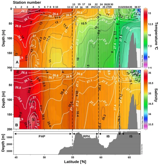
Temperature and salinity profiles overlain with isopycnals are presented in Fig. 2a and b. The southern end of the transect, from St. 1 to 13, was sampled over the PAP and was characterized by warm surface waters (0–200 m) rang-ing from 11 to 15◦C and high salinities (>35.4). A core of highly saline waters (>36) was observed at St. 4 between 150 and 200 m and may reflect an influence of Mediterranean out-flow waters. A first frontal structure was crossed at 55.5◦N at St. 14 while entering the RHP, as evidenced by a steep-ening of the 10–11◦C isotherms and of the 27.2 isopycnal, along the steep shoaling of the bottom isobaths. St. 14 to 23, located over the RHP, were characterized by colder (<11◦C) water invasions below 50 m. Stations 26 to 30 were sampled over the IB but presented similar vertical profiles to the sta-tions over the RHP. Stasta-tions 24 and 25, located above the northern slope of the RHP exhibited a slight upwelling of cooler waters (<11◦N) to the surface. From the circulation scheme proposed in Fig. 1, it can be hypothesized that St. 24– 25 may be on the main NAC trajectory exiting the RHP. The vertical temperature and density profiles between St. 26 and 30 exhibited an eddy-like structure, with a deepening of the isolines at the centre of this section.
1 2 3 4 6 10 11 12 13 14 15 16 17 18 19 20 22 23 24 25 27 28 29 3132333435 3637 7 8 5 9 21 30 26 T e m p e ra tu re °C S a lin it y A PAP RPH IB IS B Station number D e p th [ m ] Latitude [°N]
Fig. 2. Vertical sections of temperature (◦C) (A) and salinity (B) vs. latitude and bottom topography. The main regions are the Porcupine Abyssal Plain (PAP), the Rockall-Hatton Plateau (RHP), the Icelandic Basin (IB) and Icelandic Shelf (IS).
A second frontal structure was identified between St.30 and 31 (61.6◦ to 63.2◦N), with a sharp deepening of the 9.5◦C temperature and the 27.4 density isolines. Stations 31 to 37 were located over the IS and the last two stations (36–37) were characterized by a clear influence of colder (2◦C), fresher waters (salinity 34.4) from the retreat of melt-ing sea ice. The water masses encountered between St. 31 and 35 may still be characterized as MNAW according to Hansen and Østerhus (2000), which are defined by temper-atures ranging from 7 to 8.5◦C and salinities between 35.1 and 35.3 over the Greenland-Scotland ridge.
3.1.5 Mixed layer, euphotic zone and nutricline depth The depths of the mixed layer (Zm), the euphotic layer (Ze) and the nutricline (Zn) are presented in Fig. 3. Average Zm, Ze and Zn depths for each region are summarized in Table 1. The deepest euphotic layers were observed over
Table 1. Mean depths (±standard deviation) of the euphotic zone (Ze), mixed layer (Zm) and nutricline (Zn) in the PAP (Porcupine Abyssal Plain), RHP (Rockall-Hatton Plateau), IB (Icelandic Basin) and IS (Icelandic Shelf) regions.
Ze Zm Zn
PAP 56±12 m 23±10 m 48±24 m RHP 30±5 m 29±8 m 23±9 m IB 28±9 m 30±9 m 20±10 m IS 21±4 m 26±8 m 24±6 m
the PAP, between 45 and 55◦N, with an average depth of 56 m. Ze depths were shallower in the three northernmost regions (RHP, IB, IS), ranging between 21 and 28 m on aver-age. There were no significant differences in the Zmdepths
D e p th [m ] Latitude [°N] D e p th [m ] 0 20 40 60 80 100 Ze Zm Zn 1 2 3 4 6 10 11 121314 15 16 17 18192022232425 272829 3132333435 3637 7 8 5 9 21 26 30 Station number PAP RPH IB IS
Fig. 3. Depths of the euphotic zone (Ze) (1% light level), mixed layer (Zm) and nitracline (Zn) vs. latitude and bottom topography.
over the whole transect, with a shallow summer stratification signature observed between 23 and 30 m for all regions. The depths of the nutricline (calculated from DIN vertical profiles using the trapezoidal integration method between two niskin measurements) were deeper in the PAP region, with an av-erage value of 56 m, but with substantial variability between stations (from 10 to 80 m). Zn was shallower in the three northernmost regions, with an average value between 20 and 24 m and little variability between stations (from 10 to 40 m). While Zndepths were calculated from bottle data spaced ev-ery 5 to 20 m, Zm and Ze were calculated from CTD data averaged every 0.5 m. Hence, no significant correlations can be calculated between Zmand Zn.
3.2 Nutrients and trace metal distributions
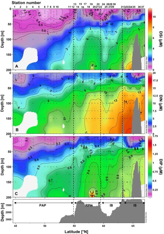
3.2.1 Major nutrients (Si, N, P) vertical distribution The vertical distributions of DSi, DIN and DIP are presented along the study transect in Fig. 4. For all nutrients, a pro-gressive shoaling of isolines towards the North was observed. The PAP was the most nutrient depleted region in early June, with DSi concentrations in surface waters as low as 0.2 µM at 46◦N (St. 2) and between 50 and 52◦N (St. 6 to 10). The 1 µM isoline was as deep as 100 m at the southern end of the transect and rose to the surface at both frontal structures, while remaining in the upper 30 m over the rest of the tran-sect. In general, surface waters were severely Si depleted while there was a constant increase in the deeper water DSi content going from South to North. A similar distribution pattern was observed for DIN and DIP, which were again most depleted in the surface layer in the PAP region and over the IS. DIN concentrations remained between 2 and 4 µM in the upper 50 m in the PAP, but decreased to 1 µM at the three
northernmost stations west of Iceland in the upper 25 m. DIP levels were below 0.2 µM in the mixed layer in the PAP as well as in the IS. Differing from DSi distribution, DIN and DIP were not as severely depleted over the RHP and the IB. All nutrient concentrations increased at the surface at the lo-cations of the two frontal structures at 55 ˚ N (St. 13) and 63.2◦N (St. 31) (Fig. 2). Furthermore, a deepening of nutri-ent concnutri-entration isolines observed at 60◦N over the IS, also seen in the density plots (Fig. 2), may indicate the presence of an anticyclonic eddy.
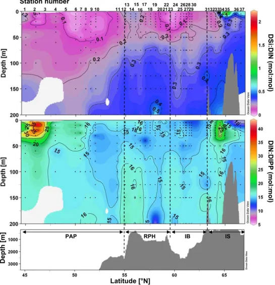
Nutrient ratios are presented in Fig. 5. The DSi:DIN plot (Fig. 5a) illustrates the severe Si depletion of the 0–200 m surface layer from 45◦N to 64.5◦N. DSi:DIN ratios in this region were well below 0.2–0.3 and close to 0 at several sta-tions (2, 6, 7, 23 and 24). In the 100–200 m layers in the northern part of the transect DSi:DIN ratios were still below 0.4. DSi only exceeded DIN concentrations at the near sur-face at two IS stations (St. 35, 37). DIN:DIP ratios were on average close to 15 over the central section of the transect, from 47.5◦to 63◦N, but exhibited higher values at the south-ern end of the transect (St. 2), with DIN:DIP ratios reach-ing 43 at 46◦N (St. 2) in the PAP. DIN:DIP ratios up to 40 were also observed in the upper 50 m over the IS at 64.5◦N (St. 34).
3.2.2 Surface trace metal distribution
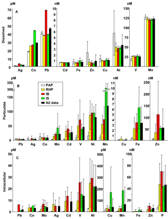
Trace metal concentrations in the dissolved, total particulate and intracellular fractions are shown in Fig. 6, with metal elements ranked in order of increasing average concentra-tions for the whole transect. In the dissolved fraction, silver (Ag), cobalt (Co) and lead (Pb) were in the picomolar range (Fig. 6a). Cobalt average concentration in surface waters was 28.6±13.6 pM for the whole transect, but averages for each
Fi Latitude [°N] D Si (µ M) D IN (µ M) D IP (µ M) A B C PAP RPH IB IS D e p th [m ] 1 2 3 4 6 10 11 12 13 14 15 16 17 18 19 20 22 23 24 25 27 28 29 3132333435 3637 7 8 5 9 21 30 26 Station number
Fig. 4. Vertical sections of (A) Dissolved silicic acid (DSi), (B) Dissolved inorganic nitrogen (NO3+NO2) (DIN) and (C) Dissolved inorganic phosphorus (DIP) in µM vs. latitude and bottom topography.
of the hydrographic regions showed a constant increase from South to North, with the lowest values in the PAP and the highest above the IS. Cadmium (Cd), iron (Fe), zinc (Zn) and copper (Cu) concentrations were fairly similar and in the nanomolar range, with respective average surface concentra-tions over the transect of 0.7, 0.8, 1.0 and 1.1 nM. Fe
sur-face concentrations were slightly higher over the IS (1.0 nM) and the PAP (0.8 nM), while Zn concentrations were high-est in the PAP (2.4 nM) but were highly variable. Both cop-per and nickel concentrations were highest in the PAP (1.4 and 5.7 nM, respectively). Vanadium (V) and molybdenum (Mo) were the most abundant dissolved metals, with average
D Si :D IN (m o l:m o l) D IN :D IPP (m o l:m o l) PAP RPH IB IS D e p th [m ] Latitude [°N] 1 2 3 4 6 10 11 12 13 14 15 16 17 18 19 20 22 23 24 25 27 28 29 3132333435 3637 7 8 5 9 21 30 26 Station number
Fig. 5. Vertical sections of (A) Dissolved Si:N ratios (mol:mol), (B) Dissolved N:P ratios (mol:mol) vs. latitude and bottom topography.
concentrations of 25.5 and 123.3 nM respectively and little variability between regions.
Total particulate metal concentrations showed a fairly dis-tinct distribution pattern, with the most abundant elements being Cu, Fe and Zn, which were in the nanomolar range (Fig. 6b). Particulate Cu concentrations were lowest and ex-hibited low variability from South to North (0.1±0.3 nM), while particulate Fe concentrations increased dramatically from South to North, from 0.4 nM in the PAP to 6.2 nM over the IS. Particulate Zn concentrations were elevated and highly variable (53.1±80.1 nM) and also increased strongly from the PAP (5.1 nM) to the IB (109.6 nM), but unlike Fe, decreased again over the IS (51.7±8.2 nM). All other partic-ulate trace metals were in the picomolar range. Some exhib-ited a steady increase northward similar to Fe (Mo, Ni and Mn), while some increased from the PAP to the IB but de-creased again over the IS, similar to Zn (Cd and V).
Intracellular metal concentrations for most elements were lower than dissolved or total particulate concentrations and were found in the picomolar range (Fig. 6c). Intracellu-lar Co and Cd concentrations were very low (3.1±2.7 pM and 8.8±8.1 pM respectively), while Cu and Mn showed a strong increase over the IS with 165.4 and 181.6 pM, respec-tively. Intracellular Fe and Zn were the only elements found in the nanomolar range, with overall average concentrations of 1.3 nM and 6.3 nM, respectively. Intracellular P from the ICP-MS analyses is indicated as well to show the evolution of biomass over each region, which resembles some trace met-als patterns of increase from the PAP to the IB and decrease over the IS.
1 2 3 4 5 6 7 8 9 10 0 10 20 30 40 50 60 70 Ag Co Pb Cd Fe Zn Cu Ni V Mo D is s o lv e d 25 50 75 100 125 150 nM nM pM PAP RHP IB IS All data Cu Fe Zn 1 2 3 4 5 6 7 8 9 10 11 50 100 150 200 250 Pa rt ic u la te pM nM nM 0 10 20 30 40 50 Pb Co Mo Ag Cd V Ni Cu Mn Fe Zn P 100 200 300 400 500 20 40 60 80 100 In tr a c e ll u la r nM pM pM A B C 0 50 100 150 350 Pb Ag Co Mo Cd V Ni Mn 300
Fig. 6. Surface trace metals concentrations averaged by regions (PAP, RHP, IB and IS) and averaged for the entire data set (All data) and standard deviation (error bars). (A) Dissolved trace metal concentrations, (B) Particulate trace metal concentrations, (C) Intracellular trace metal concentrations.
3.3 Particulate matter distribution 3.3.1 Particulate organic C, N and P
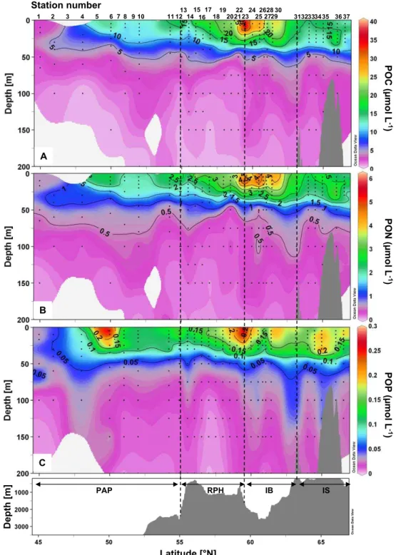
POC and PON were tightly correlated (r=0.99), and the av-erage C:N molar ratio was 5.92 (data not shown), slightly lower than the Redfield ratio (C:N=6.6). PON and POP were less well correlated (r=0.86), but the average N:P ratio for all data was 16.05 (data not shown), very close to the Red-field ratio (N:P=16). As a general trend, latitudinal transects
of POC, PON and POP (Fig. 7a, b, c) revealed a smaller ac-cumulation of biomass in the PAP region and an increase in concentrations northward, with a maximal accumulation of biomass at the surface around 59.5◦N (St. 23) at the transi-tion between the RHP and IB. Biomass in terms of POC and PON were slightly lower over the IS, while some variability was observed for the POP section with two other concentra-tions maxima at 50◦N (St. 6) and 65◦N (St. 35).
PO C (µ m o l L -1 ) PO N (µ m o l L -1 ) PO P (µ m o l L -1 ) A B C PAP RPH IB IS D e p th [m ] Latitude [°N] 1 2 3 4 6 10 11 12 13 14 15 16 17 18 19 20 22 23 24 25 27 28 29 3132333435 3637 7 8 5 9 21 30 26 Station number Fi
Fig. 7. Vertical sections of (A) Particulate Organic Carbon (POC), (B) Particulate Organic Nitrogen (PON), (C) Particulate Organic Phos-phorus (POP) in µmol L−1vs. latitude and bottom topography.
3.3.2 Pigment distribution
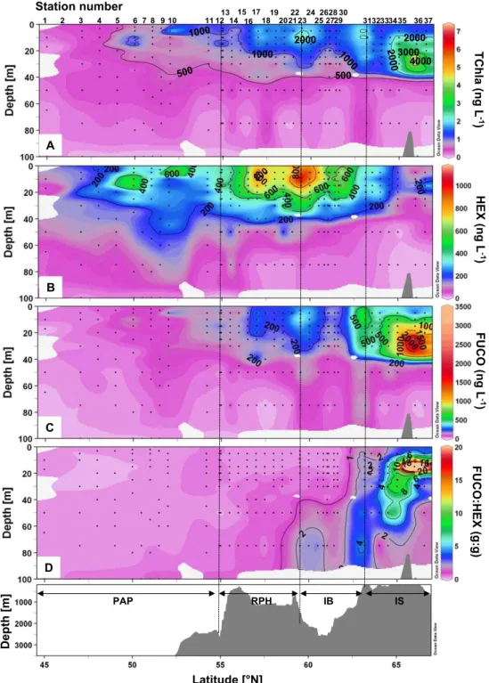
The total Chla (TChla), FUCO and HEX, and FUCO:HEX vertical distributions are presented in Fig. 8. The maximum TChla concentration was observed at the northern end of the transect at 66◦N over the IS, with 7.4 µg L−1 at 25 m
(Fig. 8a). Two smaller TChla peaks were observed at 63.2◦N and at 59.5◦N with 2.8 and 2.6 µg L−1, respectively. The dis-tribution of TChla showed a regular increase northward as well as a steady deepening of isolines. The 0.1 µg L−1 iso-line shoaled at 10 m between 52.5 and 56◦N, while reaching 50 m over the IS at 66◦N.
A T C h la (n g L -1 ) 500 500 1000 1000 10 00 2000 2000 2 0 0 0 3000 4000 PAP RPH IB IS D e p th [m ] Latitude [°N] Fi H EX (n g L -1 ) F U C O ( n g L -1 ) F U C O :H EX (g :g ) B C D 1 2 3 4 6 10 11 12 13 14 15 16 17 18 19 20 22 23 24 25 27 28 29 3132333435 3637 7 8 5 9 21 30 26 Station number
Fig. 8. Vertical sections of (A) Total Chlorophyll a (TChla) in ng L−1, (B) 19’Hexanoyloxyfucoxanthin (HEX), (C) Fucoxanthin (FUCO) in ng L−1, (D) Fucoxanthin:19’Hexanoyloxyfucoxanthin ratio (FUCO:HEX) (weight:weight) vs. latitude and bottom topography.
The two most abundant pigments measured other than Chla over the transect were 19’Hexanoyloxyfucoxanthin (HEX) and fucoxanthin (FUCO). Their vertical distributions are represented in Fig. 8b and c and the FUCO:HEX ratio in Fig. 8d. HEX is a diagnostic pigment for prymnesiophytes, including coccolithophores and Phaeocystis spp., both of
which were abundant along the transect based on onboard microscopic observations. HEX was the second most abun-dant pigment measured and was particularly abunabun-dant over the RHP and part of the IB, between 55 and 61.6◦N, with a surface maximum value of 1.2 µg L−1 located at 59.5◦N, close to the northern edge of the RHP. Two secondary peaks
were observed in the southern part of the transect over the PAP, at 50 and 52◦N. Fucoxanthin is primarily indicative of diatoms, but can also be synthesized by other chromo-phytic algal groups (e.g. Phaeocystis pouchetii), dinoflagel-lates and chrysophytes. The southern part of the transect, from 45 to 56◦N had particularly low FUCO concentrations (Fig. 10b), which increased slightly over the northern part of the RHP, with concentrations increasing to between 0.1 and 0.5 µg L−1. An intense subsurface peak of FUCO was centred above the IS, with maximum values of 3.8 µg L−1at 25 m at 66◦N, while concentrations at the surface remained low (0.2 µg L−1). At 63.2◦N (St. 31), a secondary peak of FUCO was observed and ranged from 0.5 to 0.7 µg L−1in the upper 30 m. An area of low FUCO concentrations was found over the IB around 61◦N, between the two maxima observed over the RHP and IS. The FUCO:HEX distribution reveals that HEX was the dominant pigment over most of the tran-sect from the PAP to the IB, with ratios <1 (Fig. 10c). FUCO represents the major pigment over the IS with a FUCO:HEX ratio as high as 83 at 15 m at 66◦N (St. 36). The FUCO:HEX ratio is also >1 over the IB below 50 m.
3.3.3 Distribution of biominerals: BSi (SiO2), PIC (CaCO3)
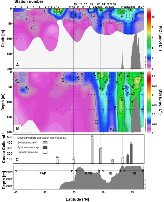
Biominerals representative of siliceous and calcareous phy-toplankton are presented in Fig. 9a and b. Particulate In-organic Carbon (PIC) here indicates the presence of cal-careous organisms such as coccolithophores since pteropods were never observed on the filters. The PIC distribution over the transect was very patchy, and except for a region of lower levels over the PAP between 45 and 50◦N, showed no clear trends with latitude (Fig. 9a). The largest accu-mulation of PIC occurred at the surface at 52◦N (St. 10), with 11.6 µmol L−1. A secondary maximum was observed over the IB, reaching 10.2 µmol L−1at 10 m depth at 63.2◦N (St. 31). Comparison between the PIC and HEX peaks lo-cated at 52◦N and 59.5◦N shows a good agreement, though discrepancies were found over the rest of the transect. A no-table peak of PIC at 63.2◦N (St. 31) was not matched by a HEX increase (Fig. 10). In contrast, there were two large HEX peaks centred at 50◦N (St. 6) and 57◦N (St. 17) that did not correspond to high PIC concentrations (Fig. 9). Hence, the overall correlation between PIC and HEX distributions was poor. The poor correlation between HEX and PIC may be explained by the presence of Phaeocystis pouchetii which was observed in bioassay experiments (data not shown) or by the presence of naked coccolithophores.
Biogenic silica distribution was very different from PIC and showed a marked increase north of 54.2◦N (St. 11) while the southern part of the transect revealed very low BSi con-centrations (Fig. 9b). The first large increase in BSi was ob-served at 59.5 and 60◦N (St. 23, 24) with concentrations ranging from 0.75 to 1.27 µmol L−1 in the upper 25 m at these two stations. A deep BSi maximum was also found
over the IB at 60.5◦N (St. 25), with a peak of 1.08 µmol L−1 at 100 m, extending to 200 m (0.45 µmol L−1). Low BSi con-centrations were again found over part of the IB between 61.04 and 61.43◦N (St. 27, 29). From 63.2◦N (St. 31) and northward, BSi was abundant from the surface to at least 200 m (concentrations below 200 m not measured). Entering the IS, a large BSi accumulation was found at 63.2◦N (St. 31) from the surface (0.86 µmol L−1) to the bot-tom of the profile (0.78 µmol L−1), with a maximum found as deep as 125 m (1.19 µmol L−1). The highest BSi accu-mulation of the transect was centred above the bathymetri-cal rise located over the IS, from 65 to 66◦N (St. 35, 36) and reached a maximum concentration of 1.61 µmol L−1 at 25 m at 66◦N, while the surface concentration at this site was moderate (0.38 µmol L−1). At the northernmost sta-tion, at 66.55◦N (St. 37), BSi showed an intense surface peak (1.12 µmol L−1at 15 m), which decreased sharply be-low 50 m (<0.16 µmol L−1). Overall, the three stations that presented the highest BSi concentrations corresponded to in-creased FUCO levels (at 59.5–60, 63.2 and 66◦N), however, FUCO was constrained within the upper 50 m, while BSi ex-tended much deeper, to at least 200 m, thus correlation was poor in the deeper water column between these two parame-ters.
3.3.4 Other taxonomic information
A few selected stations were analyzed microscopically for coccolithophore composition and abundance based on the lo-calization of the PIC maxima. These results are presented in Fig. 9c. Unfortunately, no information could be derived re-garding the two main PIC maxima at 52 and 63.2◦N (St. 10, 31) as the most abundant species could not be clearly iden-tified in scanning electron microscopy (SEM), due to a layer of material obscuring a clear view. The PIC accumula-tion over the RHP (St. 19, 23) can be attributed mainly to the presence of Emiliania huxleyi which dominated the coc-colithophore assemblage numerically, while the PIC accu-mulation measured over the IS seems to originate from a bloom of Syracosphaera spp. Other species such as
Gephy-rocapsa spp., Coccolithus pelagicus, Calcidiscus leptoporus
and Coronosphaera spp. were also present but in small abun-dance. Coccolithus pelagicus was only seen north of 58◦N (St. 19), while Gephyrocapsa spp. was only observed south of 61.43◦N (St. 29). Emiliana huxleyi was the most evenly distributed species and was observed throughout the transect.
Phaeocystis spp. was also observed on board together with
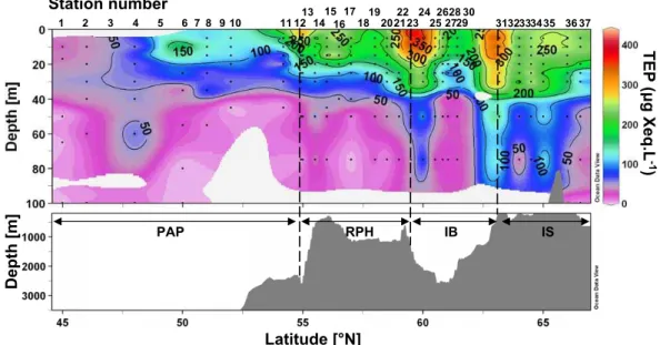
coccolithophores during bioassay experiments. 3.3.5 TEP distribution
TEP distribution is presented in Fig. 10. TEP concentrations were lowest at the southern end of the transect over the PAP, and started to increase from 50◦N (St. 5) and northward, with the highest concentrations found at both edges of the IB.
PI C (µ m o l L -1 ) B Si (µ m o l L -1 ) A
Coccolithophore population dominated by :
100 200 300 400 500 10 12 19 23 29 31 33 34 C o c c o C e ll s m l -1 Syracosphaera sp. Emiliana huxleyi Undetermined sp. C 1 2 3 4 6 10 11 12 13 14 15 16 17 18 19 20 22 23 24 25 27 28 29 3132333435 3637 7 8 5 9 21 30 26 Station number B PAP RPH IB IS D e p th [m ] Latitude [°N]
Fig. 9. Vertical sections of (A) Particulate Inorganic Carbon (PIC), (B) Biogenic Silica (BSi) in µmol L−1, (C) Coccolithophore cell counts (cells mL−1) and taxonomic information at selected PIC maxima vs. latitude and bottom topography.
Elevated TEP concentrations were measured at the surface at 55, 59.5 and 63.2◦N (St. 13, 23, 31), with concentrations ranging between 300 and 420 µg Xeq L−1. TEP were mainly found in the upper 50 m layer, but extended to 75 m on two occasions at 60 and 63.2◦N (St. 24, 31).
3.4 Integrated data
Average integrated data of diatom and coccolithophore in-dicators (BSi, FUCO, PIC, HEX) and of biomass indica-tors (TChla and POC) are presented for each provinces in
Fig. 11. We emphasize that HEX, in addition to being a marker of coccolithophore presence, may also indicate the presence of Phaeocystis pouchetii during the NASB bloom. Standard deviation bars are relatively large, highlighting the strong mesoscale variability over the transect. Integrated BSi ranged from 17.7 to 102.2 mmol m−2and increased steadily from South to North (Fig. 11a). Integrated PIC was very sim-ilar in the three southernmost provinces, despite patchy pro-files, with values ranging from 67.3 to 78.4 mmol m−2 but nearly doubled over the IS with 135.1 mmol m−2(Fig. 11a). Integrated FUCO was lowest over the PAP in the south and
T EP (μ g Xe q .L -1 ) PAP RPH IB IS Latitude [°N] 1 2 3 4 6 10 11 121314 15 16 17 18192022232425 272829 3132333435 3637 7 8 5 9 21 26 30 Station number D e p th [m ]
Fig. 10. Vertical section of Transparent Exopolymer Particles (TEP) in Gum Xanthan equivalent per Liter (µg Xeq L−1) vs. latitude and bottom topography.
highest over the IS (from 3.5 to 34.3 mg m−2), but was sim-ilar over the RHP and IB (Fig. 11b). Integrated HEX val-ues were lowest over the IS (8.2 mg m−2) and highest over the RHP (23.7 mg m−2), showing a different distribution pat-tern than PIC (Fig. 11b). Finally, integrated TChla showed a similar distribution pattern to FUCO, with lowest values over the PAP (30.7 mg m−2) and highest values over the IS (90.9 mg m−2), while integrated POC data increased steadily from the PAP to the IB (556 to 1105 mmol m−2), but de-creased again over the IS (802 mmol m−2) (Fig. 11c).
4 Discussion
4.1 Bloom development – general features
The North Atlantic bloom started in April south east of our transect near the European coasts and developed towards the northwest during May, where the spatial coverage of the bloom was largest (Fig. 12). In June, the highest concentra-tions of both surface Chla and calcite were detected, as evi-denced by the composite monthly SeaWiFs images (Fig. 12c and g). According to these satellite images, surface phyto-plankton biomass was lower over the PAP region, around the southern part of our transect, from 45◦N to 52◦N (St. 1 to 10), whereas an intense surface accumulation of both Chla and calcite was observed from the Rockall Hatton Plateau to the Icelandic shelf. Our data (Fig. 8a) was in good agreement with these global features, with low concentrations of Chla in the upper 100 m in the PAP region then increasing above 1 µg L−1from approximately 52◦N to 66.5◦N. The intense Chla accumulation south of Iceland visible on Fig. 12c
coin-cided with the slight increase of Chla surface concentrations measured at 60◦N, but the intense subsurface (25 m) Chla peak measured on the IS (Fig. 8a) was not visible on the satellite imagery, probably due to the depth of this peak. In-deed, satellites only peer through the near surface to a depth equivalent to 1/extinction coefficient. Overall, the monthly Chla composite satellite data was very well matched by our surface Chla data, both in general trends and concentrations. The calcite surface distribution was very patchy as shown in the composite image (Fig. 12g) making comparisons with in situ data difficult, but the range of concentrations observed (between 1 and 10 µmol L−1) was identical to the range of our PIC measurements (Fig. 9a). The relative absence of cal-cite at the southern end of the transect shown by the satel-lite composite was in good agreement with PIC distribution, which was below 1 µmol L−1on average in this region (south of 50◦N). The strong calcite increase visible over the north-ern half of the RHP as well as the very large peak observed over the IS were also well reproduced by our data. However, the highest PIC concentrations of the IS peak ranged between 2 and 10 µmol L−1, while satellite data showed calcite con-centrations close to 30 µmol L−1over this area. The weekly composite image from the end of the cruise (26 June–3 July 2005) corresponding closest to the sampling period of the IS stations showed reduced calcite levels, closer to 3 µmol L−1 which is in better agreement with our data. Weekly MODIS composite images (not shown) reveal that the largest coc-colithophore bloom developing west of Iceland occurred be-tween the end of May and mid-June, and was subsiding by the time we sampled the IS. It is also known that detached coccoliths can accumulate in the surface layer and that these particles have a very high reflective index, which may bias
0 250 500 750 1000 1250 1500 PAP RHP IB IS PO C (m m o l m -2) ΣPOC ΣChla 0 20 40 60 80 100 120 140 160 C h la (m g m -2 ) 0 20 40 60 80 100 120 140 160 180 200 PAP RHP IB IS m m o l m -2 ΣBSi ΣPIC 0 10 20 30 40 50 60 70 PAP RHP IB IS m g m -2 ΣHEX ΣFUCO A B C
Fig. 11. 0–200 m integrated region averages and standard deviation (error bars) of (A) Biogenic silica (6BSi) and Particulate Inorganic Carbon (6PIC) in mmol m−2, (B) Fucoxanthin (6FUCO) and 19’Hexanoyloxyfucoxanthin (6HEC) in mg m−2, (C) Particulate Organic Carbon (6POC) in mmol m−2and Total Chlorophyll a (6TChla) in mg m−2.
satellite estimations. We emphasize that comparing satellite images to in situ data is not trivial and that monthly com-posites cannot be expected to represent local sites sampled during the cruise. However, weekly images were too ob-scured by cloud cover to be useful. Our point is to show that despite potential large meso-scale features, the general trends of surface Chla and calcite measured during the cruise in terms of range of concentrations and main features could be reflected by composite satellite images. Furthermore, we show in the following section that in situ PIC and HEX data were poorly correlated, which suggest that satellite calcite data cannot be directly converted to coccolithophore abun-dance. Our cruise transect, sampled over a month, repre-sents the South-North variability of different biological and hydrological provinces but also integrates the bloom tempo-ral propagation northward. Thus, regional comparisons de-scribed below account for both spatial and temporal variabil-ity, and cannot be considered a true synoptic view of a bloom situation. Furthermore, care must be taken in extrapolating surface Chla data, which are often poorly correlated to water column integrated data, as was shown by Gibb et al. (2001) who demonstrated that conclusions derived from latitudinal differences in surface Chla were opposite to those derived from integrated Chla data.
4.2 Community structure and characteristics of the NEA phytoplankton bloom
We first present a short non-exhaustive synthesis of previous cruises carried out in the same area during spring in order to summarize the main characteristics of the spring/summer phytoplankton blooms, before comparing these studies with our results. The Biotrans site (at 47◦N, 20◦W) character-ized pigments between the end of June to mid July 1988 revealing that HEX (prymnesiophytes) was the dominant pigment for the nanoplankton size fraction while PERI
(di-noflagellates) was the major pigment in the microplankton size class (Williams and Claustre, 1991). Relatively non-degraded prymnesiophyte pigments were observed at depth, suggesting aggregation and subsequent rapid sedimentation of prymnesiophytes. One year later, Llewellyn and Man-toura (1996) sampled stations on the 20◦W meridian from 47◦N to 60◦N over the same period (first NABE cruise of JGOFS) and found that by mid-July diatoms dominated the spring bloom at 60◦N while prymnesiophytes were more im-portant at 47◦N, where the first spring bloom was already over.
The phytoplankton bloom was again sampled at 47◦N earlier in the season in 1990, and results indicated that di-atoms (23–70%) and prymnesiophytes (20–40%) dominated the Chla biomass in the first stage of the bloom during early May, while prymnesiophytes became dominant (45–55%) in the second phase from the end of May to mid-June (Barlow et al., 1993). The latter study reported a pigment maxima at 5–15 m depth with a rapid decrease below that depth in the development phase, while at the peak of the bloom, diatoms dominated throughout the water column down to 300 m. In the post-bloom phase, prymnesiophytes dominated the up-per 20 m with diatoms more abundant in deeup-per waters. The following year, in 1991, a large coccolithophore bloom was encountered south of Iceland between 60 and 61◦N, between the end of June and early July (Fernandez et al., 1993).
During the PRIME program in July 1996, the surface phy-toplankton community was dominated by prymnesiophytes between 37 and 61.7◦N, and a constant northward increase in relative diatom contribution was observed (Gibb et al., 2001). More recently, during the seasonal POMME study carried out in 2001, prymnesiophytes dominated the phyto-plankton during March and April between 39 and 43◦N ex-cept for a transition period in April when diatoms dominated at the northernmost site (43◦N) (H. Claustre, personal com-munication, 2001; Leblanc et al., 2005).
April
April MayMay JuneJune JulyJuly
A A BB CC DD E E FF GG HH A-D E-H NASB cruise 0 .0 1 0 .0 5 0 .1 0.5 1.0 Chla concentrations (mg/m3) 1 0 60 5X1 0 -5 Calcite (moles/m3) 1 X 1 0 -4 3 X 1 0 -4 5 X 1 0 -4 1 X 1 0 -3 3 X 1 0 -3 5 X 1 0 -3 1 X 1 0 -2 3 X 1 0 -2 5 X 1 0 -2 < 5 X 1 0 -5 > 6 X 1 0 -2 n o d a ta
Fig. 12. Surface monthly satellite MODIS Chla (A–D) and calcite (E–H) images obtained from the Level 3 browser at http://oceancolor. gsfc.nasa.gov/ for 2005. The black line indicates the cruise track and the framed images (C and G) the cruise sampling period (June).
The recurrent scenario emerging from these previous stud-ies is that diatoms dominate the early bloom stages, some-times co-occurring with prymnesiophytes or dinoflagellates, and tend to be outcompeted by prymnesiophytes during later stages of the spring bloom due to changing light and nutrient availability and possibly grazer control. This temporal suc-cession is also accompanied by a change in vertical phyto-plankton community structure towards the end of the spring bloom with prymnesiophytes occupying the stratified surface layer (0–30 m) while diatoms tend to dominate lower depths (30–300 m) sometimes well below the MLD.
Our observations collected during the 2005 NASB study are in good agreement with this proposed scenario. In June, we found evidence of the propagation of the spring bloom northward, with Chla increasing from the PAP region to the IS (Figs. 8a and 13c). There was a general decrease in phyto-plankton size structure from North to South, which was also observed during NABE (Sieracki et al., 1993). The pigment data showed a large prymnesiophyte bloom over both the RHP and IB, while diatoms were mostly found over the IB and IS (Figs. 10, 11 and 13b). The relative vertical distribu-tion of diatoms and prymnesiophytes along our transect was also similar to that observed during the PRIME study (Gibb et al., 2001) in that HEX dominated the surface layer, while FUCO:HEX ratios >1 were found below 50 m (Fig. 10c).
Overall, the correlation between HEX and PIC was very poor for the entire cruise and may reflect a large contribution of Phaeocystis pouchetii, wherever HEX was not associated with PIC accumulation (St. 6, St. 27 to 30) and the tempo-ral mismatch between coccolithophore biomass and coccol-ith concentration. Another explanation would be the pres-ence of naked coccolithophores, but we have no data to sub-stantiate this hypothesis.
The former reason is confirmed in Table 2, which sum-marizes the significance of correlations between the di-atom and prymnesiophyte/coccolithophore indicators (BSi, FUCO, PIC, HEX) with the other main biogeochemical vari-ables such as nutrients and biomass data. The PIC data stand out in this table as the one parameter that is most poorly cor-related to any of the other variables. PIC and HEX were never significantly correlated and this is true regardless of testing the whole data set or testing each region separately. A poor correlation was also found in another study in the North Atlantic for a global data set (n=130) on the same transect from 37◦N to 59◦N, with significant PIC-HEX correlations found only for underway data and for data collected at 59◦N (but for a very small data subset, n=11) (Gibb et al., 2001).
These results emphasize the difficulties in using bulk pigment and mineral indicators for a group such as coc-colithophores. Both the cellular biomineral and pigment
Table 2. Spearman-rank correlation coefficients (rs) calculated for the diatom and coccolithophore bulk indicators (BSi, FUCO, PIC, HEX) with the other main biogeochemical data for the complete data set (All) and each region (PAP, RHP, IB and IS). Correlations are considered significant when p<0.01 (two-tailed). Degrees of freedom were comprised between 132 and 243 for all regions, between 27 and 64 for the PAP region, between 45 and 124 for the RHP region, between 22 and 57 for the IB region and between 31 and 63 for the IS region. Non-significant correlations are indicated in italic, and strong correlations (rs>0.5 or <−0.5) are indicated in bold.
DSi DIN DIP NH4 FUCO HEX TEP POC PON POP PIC BSi TChla
All BSi ns ns ns 0.279 0.794 0.234 0.623 0.463 0.412 0.520 0.306 – 0.607 Fuco −0.289 −0.358 −0.316 0.185 – 0.615 0.801 0.698 0.677 0.799 0.428 0.794 0.921 PIC ns ns ns ns 0.428 ns 0.396 0.285 0.280 0.390 – 0.306 0.420 HEX −0.507 −0.391 −0.386 ns 0.615 – 0.580 0.729 0.679 0.670 ns 0.234 0.746 PAP BSi −0.343 ns ns 0.404 0.599 0.129 ns ns ns 0.308 ns – ns Fuco −0.684 −0.545 0.478 ns – 0.876 0.478 0.860 0.838 0.778 ns 0.599 0.904 PIC ns ns ns ns ns ns ns ns ns ns – ns ns HEX −0.818 −0.728 −0.677 ns 0.876 – 0.655 0.777 0.827 0.834 ns ns 0.949 RHP BSi −0.562 ns −0.406 ns 0.802 0.579 0.490 0.640 0.532 0.646 ns – 0.630 Fuco −0.793 −0.675 −0.567 ns – 0.871 0.722 0.733 0.620 0.827 0.381 0.802 0.906 PIC ns ns ns ns 0.381 ns ns ns ns ns – ns 0.396 HEX −0.740 −0.713 −0.638 ns 0.871 – 0.830 0.862 0.772 0.874 ns 0.579 0.944 IB BSi −0.505 ns −0.371 ns 0.746 0.431 0.647 0.391 ns 0.366 ns – 0.464 Fuco −0.511 ns −0.439 ns – 0.846 0.893 0.785 0.734 0.709 ns 0.746 0.890 PIC ns ns ns ns ns ns ns ns ns 0.652 – ns 0.540 HEX −0.560 −0.494 −0.605 ns 0.846 – 0.855 0.907 0.899 0.845 ns 0.431 0.974 IS BSi ns ns ns ns 0.563 ns 0.536 ns ns 0.423 ns – 0.545 Fuco −0.438 −0.561 −0.598 ns – ns 0.670 0.692 0.649 0.815 ns 0.563 0.950 PIC ns ns ns ns ns ns ns ns ns ns – ns ns HEX −0.417 −0.494 ns −0.547 ns – 0.404 0.434 0.424 ns ns ns ns
contents are highly variable and depend on the cell’s phys-iological status and species. During their growth, particu-larly in senescence, some coccolithophores shed their coc-coliths. These coccoliths are too small to sink and tend to accumulate in the surface layer. This further decouples PIC from the biomass of living coccolithophores. For in-stance, the remnants of a coccolithophore bloom is indicated by the presence of PIC in the surface layer from St. 31 to 35 over the IS, but with no HEX accumulation, likely reflect-ing the presence of detached coccoliths while pigments and organic carbon have been lost, e.g. sedimented, degraded or grazed. Surface increases in HEX without similar PIC ac-cumulation were also observed (for instance at St. 17) and could indicate the presence of either uncalcifying strains of coccolithophores or more likely an increased contribution of
Phaeocystis pouchetii. The correlation between PIC with
HEX, even though not significant, increased slightly over the RHP and IB regions (rs=0.36 and 0.44, respectively) where it can be hypothesized that the contribution of coc-colithophores vs. Phaeocystis pouchetii increased.
BSi and FUCO concentrations were on the other hand al-ways significantly correlated (Table 2), with correlation co-efficients (rs) of 0.56 to 0.80. The entire data set showed a very strong correlation with an rs value of 0.79, which was also very high over the RHP (0.80) and the IB (0.75). Slightly
lower coefficients were found over the PAP (rs=0.59) and IS (rs=0.56). These weaker correlations can be explained by the presence of more senescent cells with low pigment con-tents or empty diatom frustules. This was most likely the case over the IS where high BSi concentrations extended as deep as 200 m (Fig. 9b), well below the Zedepth of ∼20 m (Fig. 3), while most of the Chla was confined to the first 50 m (Fig. 8a). Hence it is unlikely that diatoms were still grow-ing as deep as 200 m and this signal more probably represents sinking diatoms. This is further confirmed by phaeophyllides concentrations (data not shown), which were much higher in the IB and IS regions than in the PAP and RHP regions. Some interference with lithogenic silica (LSi) near bottom (75 m only at St. 35 and 36) could also have occurred since BSi data were not corrected for LSi during analysis.
Phaeocys-tis spp. is also known to produce FUCO (Schoemann et al.,
2005) and could explain differences between BSi and FUCO comparisons. However, in our study, the presence of FUCO was always matched by the presence of BSi, and we often ob-served the presence of BSi without FUCO. Hence, it is likely that in our study FUCO was mostly indicative of diatoms.
More surprisingly, FUCO and HEX were highly correlated during our survey in the PAP, RHP and IB regions (rs=0.88, 0.87 and 0.85, respectively) but not over the IS, where FUCO was overall dominant. Even though FUCO concentrations