HAL Id: insu-02269704
https://hal-insu.archives-ouvertes.fr/insu-02269704
Submitted on 23 Aug 2019HAL is a multi-disciplinary open access
archive for the deposit and dissemination of sci-entific research documents, whether they are pub-lished or not. The documents may come from teaching and research institutions in France or abroad, or from public or private research centers.
L’archive ouverte pluridisciplinaire HAL, est destinée au dépôt et à la diffusion de documents scientifiques de niveau recherche, publiés ou non, émanant des établissements d’enseignement et de recherche français ou étrangers, des laboratoires publics ou privés.
Risky future for Mediterranean forests unless they
undergo extreme carbon fertilization
Guillermo Gea-Izquierdo, Antoine Nicault, Giovanna Battipaglia, Isabel
Dorado-Liñán, Emilia Gutiérrez, Montserrat Ribas, Joel Guiot
To cite this version:
Guillermo Gea-Izquierdo, Antoine Nicault, Giovanna Battipaglia, Isabel Dorado-Liñán, Emilia Gutiér-rez, et al.. Risky future for Mediterranean forests unless they undergo extreme carbon fertilization. Global Change Biology, Wiley, 2017, 23 (7), pp.2915-2927. �10.1111/gcb.13597�. �insu-02269704�
1 Risky future for Mediterranean forests unless
1
they undergo extreme carbon fertilization 2
Running head: Mediterranean forests, climate change and CO2 3
1G Gea-Izquierdo, 2A Nicault, 3,4G Battipaglia, 1I Dorado-Liñán, 5E, Gutiérrez, 5M
4
Ribas, 6J Guiot
5
1,7INIA-CIFOR. Ctra. La Coruña km. 7.5 28040 Madrid, Spain. 2Aix-Marseille
6
Université/CNRS FR 3098 ECCOREV 13545 Aix-en-Provence, France. 3Department of
7
Environmental, Biological and Pharmaceutical Sciences and Technologies Second
8
University of Naples Via Vivaldi, 43 - 81100 Caserta, Italy. 4Ecole Pratique des
9
Hautes Etudes (PALECO EPHE), Institut des Sciences de l'Evolution, University of 10
Montpellier 2, F-34090 Montpellier, France. 5Departament 4Departament d’Ecologia, 11
Universitat de Barcelona, Avda. Diagonal 643, 08028 Barcelona, Spain. 6Aix-Marseille
12
Université/CNRS/IRD UM 34, CEREGE 13545 Aix-en-Provence. 7Corresponding
13
author: phone 0034913471461; email [email protected]
14 15
Abstract 16
Forest performance is challenged by climate change but higher atmospheric [CO2] (ca)
17
could help trees mitigate the negative effect of enhanced water stress. Forest projections 18
using data-assimilation with mechanistic models are a valuable tool to assess forest 19
performance. Firstly, we used dendrochronological data from 12 Mediterranean tree 20
species (6 conifers, 6 broadleaves) to calibrate a process-based vegetation model at 77 21
sites. Secondly, we conducted simulations of gross primary production (GPP) and radial 22
growth using an ensemble of climate projections for the period 2010-2100 for the high-23
emission RCP8.5 and low-emission RCP2.6 scenarios. GPP and growth projections 24
were simulated using climatic data from the two RCPs combined with: (i) expected ca;
2 (ii) constant ca = 390 ppm, to test a purely climate-driven performance excluding
26
compensation from carbon fertilization. The model accurately mimicked the growth 27
trends since the 1950s when, despite increasing ca, enhanced evaporative demands
28
precluded a global net positive effect on growth. Modeled annual growth and GPP 29
showed similar long-term trends. Under RCP2.6 (i.e. temperatures below +2ºC with 30
respect to preindustrial values) the forests showed resistance to future climate (as 31
expressed by non-negative trends in growth and GPP) except for some coniferous sites. 32
Using exponentially growing ca and climate as from RCP8.5, carbon fertilization
33
overrode the negative effect of the highly constraining climatic conditions under that 34
scenario. This effect was particularly evident above 500 ppm (which is already over 35
+2ºC), which seems unrealistic and likely reflects model miss-performance at high ca
36
above the calibration range. Thus, forest projections under RCP8.5 preventing carbon 37
fertilization displayed very negative forest performance at the regional scale. This 38
suggests that most of western Mediterranean forests would successfully acclimate to the 39
coldest climate change scenario but be vulnerable to a climate warmer than +2ºC unless 40
the trees developed an exaggerated fertilization response to [CO2].
41 42
Keywords: Dendroecology; process-based models; carbon fertilization; climate change; 43
MAIDEN; water stress; forest dynamics. 44
Type of paper: Original research article 45
3 Introduction
46
Future climate will trigger changes in ecosystem functioning, including 47
enhancement in forest vulnerability to water stress (Giorgi & Lionello 2008; van der 48
Molen et al. 2011; Anderegg et al. 2015). Understanding how forests will respond to 49
warmer conditions but under higher than present ca is crucialto assess future forest
50
performance. Theoretically,plants should enhance growth and net primary productivity
51
(NPP) by optimization of different functional traits in response to elevated [CO2] (i.e. ca
52
levels way above present values, eCO2) if this was a limiting factor. In practice, rising ca
53
has enhanced intrinsic water-use efficiency (iWUE) in forests but this was not generally
54
translated on a net increase of growth, meaning that other factors such as water stress
55
and/or nutrient limitation have overridden the potential positive effect of CO2 (Peñuelas
56
et al. 2011; Keenan et al. 2013; Reichstein et al. 2013; van der Sleen et al. 2014; Kim et 57
al. 2016). 58
The net effect on tree growth of the interaction ‘Climate x CO2’ can depend
59
nonlinearly on ca levels (Reichstein et al. 2013). Observational data show evidence up
60
to current ca < 403 ppm whereas future emission scenarios project ca far above this level
61
(IPCC 2014). Free-Air Carbon dioxide Enrichment (FACE) experiments were designed
62
to address this issue. In these experiments [CO2] was elevated up to 600-800 ppm but
63
they were carried out under current environmental conditions mostly on temperate
64
forests (Battipaglia et al. 2013; De Kauwe et al. 2013; Baig et al. 2015; Kim et al. 2016;
65
Norby et al. 2016). Thus, the effect of eCO2 on forest performance in relation to climate
66
and other environmental factors needs to be addressed in other biomes where more
67
constraining (warmer and drier) conditions are expected for the future (Giorgi &
68
Lionello 2008; García-Ruiz et al. 2011; IPCC 2014). The role that CO2 could play to
69
compensate the negative impact of increasing water stress on forests has long been 70
4 debated. Plants can coordinate different functional traits in response to eCO2 and 71
drought-prone species at dry sites could benefit more from eCO2 (Medlyn & De Kauwe
72
2013; Duursma et al. 2016; Kelly et al. 2016). Leaf-level responses are easier to predict 73
than canopy or ecosystem-level responses (Fatichi et al. 2015). Consequently, there is 74
still uncertainty on how the forest carbon cycle will adjust in the future because multiple 75
interactive factors determine the net response of forests at different scales (Breda et al. 76
2006; Niinemets 2010; van der Molen et al. 2011; Kattge et al. 2011). 77
Vegetation models combine the effect of different stress factors on different 78
functional traits to achieve a proper understanding of forest functioning. These models 79
should be able to combine C-sink and C-source limitations to provide key information 80
on how forests will develop in the future (Sala et al. 2012; McDowell et al. 2013; 81
Fatichi et al. 2014; Anderegg et al. 2015; Walker et al. 2015). There is a constant need 82
to improve the representation of hydrological, physical and biological processes in 83
models. In addition, improvement of model performance needs to be achieved through 84
benchmarking and data-assimilation (Peng et al. 2011; Pappas et al. 2013; Medlyn et al. 85
2015; Prentice et al. 2015). Dendrochronological data have long been used to assess 86
empirical relationships between climate and growth, which can be used as an indicator 87
of tree fitness and performance (Fritts 1976). Process-based models can take into 88
account the influence of CO2 on plant functional acclimation. Thus they can help to
89
reduce uncertainty in growth projections but need continuous feedback from multiproxy 90
data to ensure realism (Guiot et al. 2014; Walker et al. 2015). Dendrochronological 91
records can be used to improve complex process-based models and help to assess forest 92
dynamics under global change (Babst et al. 2014). Assessing forest dynamics is 93
particularly challenging in ecosystems like those under Mediterranean climate (Morales 94
et al. 2005) where two stress periods (cold in winter and drought in summer) limit plant
5 performance. Warmer winters could enlarge the growing season and promote higher 96
photosynthetic rates (just in evergreens) but also higher respiration rates, whereas 97
warmer summers would exert a negative impact (higher water stress) on forests. 98
Modeling the net effect on trees of the balance between these two periods is critical to 99
assess the future forest response to climate change. 100
We analyzed the effect that forthcoming changes in climate and ca will yield over
101
Mediterranean forests, which are expected to face a high vulnerability to future climate 102
(Giorgi & Lionello 2008; García-Ruiz et al. 2011; IPCC 2014). We calibrated a stand
103
mechanistic model using a network of tree-ring growth chronologies including an 104
ensemble of species covering a wide ecological and geographic range to ensure realism
105
and biological robustness when simulating future forest performance at the regional
106
scale under different climate and ca scenarios. C-assimilation and C-allocation were 107
explicitly controlled by climate and CO2 at different phenological stages (Misson 2004;
108
Gea-Izquierdo et al. 2015). Importantly, the model includes a C storage pool to take into 109
account carry-over effects and its daily scale can fit different limiting environmental 110
conditions at different periods within and among years (Sala et al. 2012; Fatichi et al. 111
2014). Thus, the net effect in response to the winter and summer stress periods was 112
explicitly assessed. Forest projections were implemented using two contrasting 113
representative concentration pathways (RCPs, van Vuuren et al. 2011). Using model 114
simulations of future forest growth and GPP we addressed the following questions: (i) 115
what will be the net effect of a warmer climate for Mediterranean forests?; (ii) to what 116
extent could rising ca help compensate the expected negative effect of climate warming
117
on forest growth and productivity? (iii) how will Mediterranean forests perform in 118
relation to the maximum temperature threshold for future climate (i.e. +2.0ºC respect to 119
preindustrial levels) agreed in the COP21 (http://www.cop21paris.org/)?
6 121
Material and Methods
122
Forest sites: growth data for model calibration 123
To calibrate the model at the regional scale we used dendrochronological data from
124
77 forest sites including 12 Mediterranean tree species: 6 conifers and 6 broadleaves
125
(App. 1). These data were either owned by the authors or obtained from databases
126
(ITRDB,
https://www.ncdc.noaa.gov/data-access/paleoclimatology-data/datasets/tree-127
ring; DendroDB, https://dendrodb.eccorev.fr/framedb.htm). We explored the data to
128
avoid chronologies where major site disturbances could have affected the
decadal-to-129
multidecadal growth variations. The chronologies included were older than 80 years in
130
order to avoid the effect of juvenile growth (data used for calibration started in 1950)
131
and ended later than 1995. Exceptionally, some sites ending before 1995 in Algeria
132
were included to ensure enough data from that region. The resulting calibration period
133
slightly differed across sites due to the different time-span of chronologies, but always
134
fell between 1950 and 2010 and was greater than 40 years. For the analysis, ring-width
135
growth data were transformed to basal area increments (BAI, cm2 year-1). One output 136
from the model is C allocated to the tree stem (g C m-2 year-1). To make BAI and model
137
output comparable for model calibration both data were normalized to unitless indices
138
(Misson 2004; Gaucherel et al. 2008).
139 140
Climate and ca: historical data and future scenarios
141
Daily precipitation and temperature data used for model calibration for 1950-2010
142
were either obtained from http://www.meteo.unican.es/datasets/spain02 (Herrera et al.,
143
2012) for Spain (20 km grid) or from http://hydrology.princeton.edu/data.php (Sheffield
144
et al. 2006) for the rest (1º grid). Data were downscaled to match mean climatic local 145
7
values where these were available. For the future forest projections we used two
146
greenhouse gas (GHG) radiative forcing scenarios developed for the Fifth Report of the
147
IPCC (IPCC 2014), called RCPs (Van Vuuren et al. 2011). RCP8.5 (GHGRF<8.5
148
W/m2) is the “business as usual” scenario. RCP2.6 is the most optimistic and stringent
149
among RCPs, corresponding to strong mitigation policies with a GHG radiative forcing
150
constrained to remain <2.6 W/m2. RCP2.6 is the only RCP limiting global warming to
151
+2°C relative to the pre-industrial level. We used a multimodel ensemble of 19
152
simulations for RCP2.6 and 18 simulations for RCP8.5 performed by 13 climatic
153
institutes (see App. 2). The global climate models have a coarse resolution, from one to
154
more than five degrees depending on the model. There is often some mismatch between
155
the stand level and input climatic data (Körner 2003; Potter et al. 2013; Pappas et al.
156
2015). This was minimized as possible by downscaling climate scenarios to match the
157
shared period of the historical data. Under RCP8.5 the projected climate for our study
158
sites describes a relative increase in mean annual temperature (MAT) of +5.0ºC and a
159
decrease of over 40% in mean annual precipitation (MAP) by 2100 respect to current
160
values. Under RCP2.6 the projected climate forecasts a mean increase in MAT of
161
+1.0ºC by 2068, stabilizing thereafter, with no decrease in MAP respect to current
162
conditions (App. 3).
163 164
The process-based model MAIDEN 165
The vegetation model MAIDEN (Fig. 1) was originally developed to be used with
166
dendrochronological data by being calibrated to both time series of radial growth and
167
estimates of transpiration from sap-flow experiments (Misson 2004). Recently, the
168
model has been further developed to be used with evergreen Mediterranean taxa with a
169
multiproxy approach using gross primary productivity (GPP) estimates from Eddy
8
covariance stations and plot growth data (Gea-Izquierdo et al. 2015). Inputs are daily
171
climatic data (precipitation, maximum and minimum temperatures) and ca. In addition
172
173
Fig. 1. Outline of MAIDEN. Only GPP (gross primary production) and biomass
174
allocated to the stem (used to calibrate the model sitewise) estimates (blue boxes) are
175
reported along the manuscript. Daily output of each variable is generated based on the
176
input data of day i. ‘Weather’ corresponds to daily integrals of precipitation as well as
177
maximum and minimum daily temperatures. GPP and ‘Stomatal conductance’ are
178
functions of CO2, whereas variability within the other processes is mostly driven by 179
meteorological inputs directly or indirectly (e.g. SWC). For more details on the
180
functions and processes outlined see Misson (2004) and Gea-Izquierdo et al. (2015).
181 182
the model requires as input different site related physiographic characteristics and
183
species functional traits (see Gea-Izquierdo et al. 2015 for details). The processes within
184
the model are mainly functions of climate, CO2 and soil water availability (hence water
9
stress). The model acts at the stand level calculating carbon and water fluxes (Fig. 1)
186
using a coupled photosynthesis-stomatal conductance model. It uses the standard
187
biochemical model of Farquhar et al. (1980) in which photosynthesis is driven by the
188
most limiting between Rubisco-limited activity and electron-transport. Stomatal
189
conductance is also estimated using a widely used equation as a function of vapor
190
pressure deficit (VPD, Leuning 1995). After GPP and autotrophic respiration have been
191
estimated carbon is allocated to different tree components. Photosynthesis and
192
allocation are driven by decoupled non-linear (daily) functions of climate. Thus growth
193
is not only a direct function of C availability and the model is designed to address in
194
time not only C-source but also C-sink limitations, which is an important step required
195
to achieve more robust and realistic vegetation models (Muller et al. 2011; Sala et al.
196
2012; Fatichi et al. 2014). The model is particularly sensitive to water stress by
197
implicitly modeling as functions of climate and water stress some functional and
198
demographic traits such as leaf area, carbon allocation, leaf- and canopy-level
199
photosynthesis and transpiration (Muller et al. 2011; Gea-Izquierdo et al. 2015;
200
Duursma et al. 2016; Kelly et al. 2016). [CO2] only affects photosynthesis and stomatal
201
conductance, i.e. leaf area or respiration are direct functions of climate but not CO2. A
202
brief outline of the model is shown in Fig. 1.
203 204
Model calibration and ecological coherence of the parametric space 205
Calibration of complex multiparametric models is necessary to improve model
206
performance and because of the presence of collinearities between parameters and
207
absence of an exact solution (Prentice et al. 2015). To ensure good model performance,
208
it is important to assess the functional coherence of parameters to be calibrated. In
209
addition to calibration, it is desirable to run independent validations particularly when
10 models are fitted for prediction purposes. Nevertheless, we could not run an 211
independent crossvalidation for two reasons: (1) we calibrated against annual growth 212
(i.e. we had a number of observations between 40 and 60) estimates by integrating 213
annually the daily estimates from the model, therefore our data was too short to be split 214
in two, (2) a jackknife was intractable both computationally and also because 215
continuous (daily) time data series are needed to run the model, i.e. in case individual 216
years were left out the model could not calculate the carbon and water dynamics needed 217
to compute the complete time series at each site.
218
We implemented a species-specific approach rather than using plant functional
219
types (PFTs) as it is often applied in ecosystem models (Kattge et al. 2011; Atkin et al.
220
2015; Pappas et al. 2016). We applied the model at the regional scale and to different
221
species to analyze forest performance under future climate and ca. Data-assimilation 222
was used to apply the model to different ecological conditions and species (Peng et al.
223
2011; Medlyn et al. 2015). Overall, the growth data did not show a positive trend
224
whereas ca increased steadily in the calibration period (1951-2010). Therefore, by
225
calibrating the model site-wise using non-detrended (but normalized) growth data and
226
observed ca levels we assured that the model excluded an artificial carbon fertilization
227
effect on past growth. Additionally, to avoid overestimation of photosynthesis and get
228
unbiased simulations (Schaefer et al. 2012), we ensured that maximum GPP daily
229
integrals yielded within ranges given in Baldocchi et al. (2010): 4-6 g C m-2 day-1 for
230
evergreens and of 10-14 g C m-2 day-1 for deciduous species. Similarly, we constrained
231
annual GPP and NPP estimates to be within those measured for similar ecosystems (see
232
Table 3 in Falge et al. 2002 and Table 3 in Luyssaert et al. 2007). Species Specific leaf
233
area (SLA) was obtained from Mediavilla et al. (2008) and Kattge et al. (2011).
11
Here, within the processes in Fig. 1 we show those functions with parameters
235
involved in the calibration phase. For more details, we refer to the original model in
236
Misson (2004) and the updated modified last version in Gea-Izquierdo et al. (2015).
237
(i) "#(%) =()*+,(-./0 (
1·(345(/)6-./078)) [E1] 238
(ii) =>((i) = (1 − exp (D>E./-F · GHI(%)) · Jexp J−0.5 · NOPQR(/)6STUVP8
STWX Y
Z
[[ [E2] 239
(iii) =>Z(i) = (1 − exp (]^>E./-F· GHI(%)) · _exp _−0.5 · JOPQR-F(/)6-FTUVP8
TWX_UVP8 [
Z
aa [E3] 240
(iv) =c(i) = d1 − exp (]^cFeES· fEgh(%)i · _exp _−0.5 · J-F345(/)
jWX_Pk7WU[
Z
aa [E4] 241
"# is a soil water stress function affecting stomatal conductance. a31, a32 and a4 are
242
allocation functions for two different phenological periods (3 and 4). a31 is related to the
243
leaves and a32 tothe stem, whereas a4 determines C allocation between the stem and 244
storage. SWC is soil water content and Tmax is daily maximum temperature. We
245
calibrated soilip from [E1]; D>E./-F and D>FeES from [E2]; ]^>E./-F and ]^>FeES from
246
[E3]; and ]^c-m_E./-F and ]^cFeES from [E4]. The rest of parameters were set following
247
Gea-Izquierdo et al. (2015). All parameters except soilip (which is related to the
248
stomatal response) help to define carbon allocation in relation to soil water content and
249
air temperature during the active period.
250
We calibrated these model parameters taking into account variability in functional
251
traits and the response to climate of plant processes related to site and species. To
252
address the local phenotypic response of species (Montwé et al. 2016), some of those
253
parameters (≤7) described in the previous paragraph were calibrated site-wise using
254
maximum likelihood principles and a global optimization algorithm (Gaucherel et al.
255
2008; Gea-Izquierdo et al. 2015). A maximum of 7 allocation parameters from [E1] to
256
[E4] were optimized depending on species by comparing normalized annual integrals of
12
modeled C allocation to the stem and normalized annual growth series. We calculated
258
different statistics to check the goodness of fit: the coefficient of determination (R2), the
259
linear correlation (ρ), and the correlation (rlow) between filtered (using splines with a 260
50% frequency cutoff of 30 years) observed and modelled growth. rlow was calculated to
261
analyse the model capability to mimic the interannual and decadal growth trends. To
262
discuss the validity of our modelling exercise and since we could not run an
263
independent verification to the calibration conducted, coherence of the intersite
264
multiparametric space was analysed by exploring the ecological significance of
265
parameters compared to different site characteristics including latitude, longitude,
266
altitude, precipitation, temperature, and Penman-Monteith potential evapotranspiration
267
(PET), which was calculated for each site following Allen et al. (1998). The
268
relationship between the 7 model parameters fitted at each of the 77 sites and the mean
269
site ecological covariates was explored through pointwise correlations: (i) using site 270
individual indices; (ii) using the principal components (PCs) of the 7 x 77 matrix 271
(Legendre & Legendre 1998). 272
273
Forest performance under climate change and different ca scenarios
274
Once the model had been calibrated we implemented forest projections at the 77
275
sites using simulated climatic data generated under RCP2.6 and RCP8.5. To discuss the
276
effect of ca on the net response of forests to climate change we compared two type of
277
forest simulations driven by the multimodel climatic scenarios:
278
(i) ‘fertilization’ scenario: with ca levels expected for RCP2.6 and RCP8.5.
279
(ii) ‘non-fertilization’ scenario: using climate from RCP2.6 and RCP8.5 but constant ca
280
= 390 ppm after 2010.
281
We report GPP in addition to growth projections. Future growth trends were assessed
13
Group n R2 r rlow
Mean (sd) Max (Min) Mean (sd) Max (Min) Mean (sd) Max (Min)
Broadleaves 22 0.343 (0.168) 0.643 (0.0) 0.675 (0.084) 0.821 (0.483) 0.728 (0.185) 0.929 (0.114)
Conifers 55 0.356 (0.141) 0.710 (0.073) 0.676 (0.070) 0.855 (0.537) 0.786 (0.156) 0.968 (0.249)
Total 77 0.353 (0.148) 0.710 (0.0) 0.675 (0.074) 0.855 (0.483) 0.769 (0.165) 0.968 (0.114)
Table 1. Mean values of goodness of fit statistics. n= number of forest sites; R2=coefficient of determination; r=coefficient of correlation;
283
rlow=coefficient of correlation of filtered data (see material and methods for details).
284
285
Fig. 2. Map showing the coefficient of determination (R2) and correlation (ρ) between dendrochronological data and modeled stem growth data
286
using MAIDEN at the 77 forest sites. R2 is shown in (a) whereas ρ in (b). For R2 we split in four classes: 0≤R2<0.15; 0.15≤ R2<0.3; 287
0.3≤R2<0.45; 0.45≤ R2. For ρ in: 0.45≤ ρ <0.5; 0.5≤ ρ <0.6; 0.6≤ ρ <0.7; 0.7≤ ρ. Triangles depict conifers, whereas circles broadleaves. 288 -10 -5 0 5 10 15 20 30 32 34 36 38 40 42 44 46 48 Broadleaves Conifers Europe Africa N Mediterranean Sea Longitude Lat itu de R2 <0.15 <0.3 <0.45 >0.45 (a) -10 -5 0 5 10 15 20 30 32 34 36 38 40 42 44 46 48 Broadleaves Conifers Europe Africa N Mediterranean Sea Longitude Lat itu de ρ <0.5 <0.6 <0.7 >0.7 (b)
14
through the slope of simple regressions between simulated growth (or GPP) for a given
289
scenario and site against year for the periods 2010-2100, 2010-2050 and 2051-2100.
290 291
Results
292
Model calibration across western Mediterranean forests 293
The model fit against the calibration data is shown in Fig. 2 and Table 1 and the
294
parameters fitted in App. 4. Importantly, data used to calibrate the model did not show
295
an overall significant increase in growth, hence did not suggest evidence of a global net
296
carbon fertilization effect during the last decades (Table 2). The observed growth trends
297
were highly correlated with the model output (ρ and particularly rlow in Table 1). 298
Correlation between model output (carbon allocated to the stem) and growth data was in
299
average 0.67 whereas mean R2 was 0.36 (Table 1). The multiparametric space of the 77
300
fitted models was explored through PCA. The eigenvalues corresponding to the three
301
first principal components (PCs) were over the mean, hence significant according to the
302
Kaiser-Guttman criterion (Legendre & Legendre 1998). These three PCs including the 7
303
parameters fitted in the calibration phase explained 60.9 % of the variability (PC1 24.7
304
%, PC2 19.7 % and PC3 16.6%). PC1 was mostly related to parameters linked to
305
humidity: a positive relation with moisture parameters such as soilip and !"#$%_'()$*, and
306
a negative one with !"+'()$* (not shown). PC2 was mostly related to parameters linked
307
to temperatures: positively with !"#*,'- and negatively with .+*,'- and !"+*,'-. PC3
308
was positively correlated with the humidity parameter .+'()$* (not shown). The 77
309
parameters and the PCs (2 and 3) showed some significant relationships with the site
310
ecological characteristics (Fig.3). Most of the site-based relationships between the fitted
311
parameters and the ecological characteristics of the 77 sites were linked to site
312
temperatures (Fig. 3), whereas almost no significant relationships were found with the
15
other tested covariates (e.g. site precipitation or PET). These relationships suggest the
314
existence of some ecological coherence within the parametric space fitted for the 77
315
forest sites, which would support the robustness of the model parameterization used.
316
317
Fig. 3. Ecological coherence of model parameters at the 77 forest sites (only those
318
relationships that were significant are shown): (a) PC2 and site Tmax; (b) PC3 and site
319
Tmin; (c) st3temp and site Tmin. 320
321
Growth-GPP projections under changing climate and ca
322
The model allocates carbon to different plant compartments driven by different
non-323
linear functions of environmental variability, hence it allows some decoupling between
324
GPP, NPP and secondary growth. In this sense, 59% and 80% of the simulations
325
presented correlations between GPP and growth higher than 0.5 for RCP2.6 and
326
RCP8.5, respectively (App. 5). Thus the majority of sites showed a good agreement
327
between interannual GPP and growth (i.e. generally the modeled interannual variability
328
of growth was driven by that of GPP). Furthermore, the growth trends (long-term,
329
multiannual) were of similar sign (positive, negative or neutral) as those of GPP (Table
330 sitios_red2$Tmax p ec es _p ar [, 2] ρ = 0.258p = 0.023 (a) -3 -2 -1 0 1 2 3 14 16 18 20 22 24 -3 -2 -1 0 1 2 sitios_red2$Tmin p ec es _p ar [, 3] ρ = -0.290 p = 0.010 (b) 2 4 6 8 10 12 14 16 -200 -100 0 100 200 sitios_red2$Tmin p ar s_r ed _f3$b u d _tmax ρ = -0.287 p = 0.011 (c) Tmin(ºC) Tmax(ºC) st 3te m p P C 3 P C 2
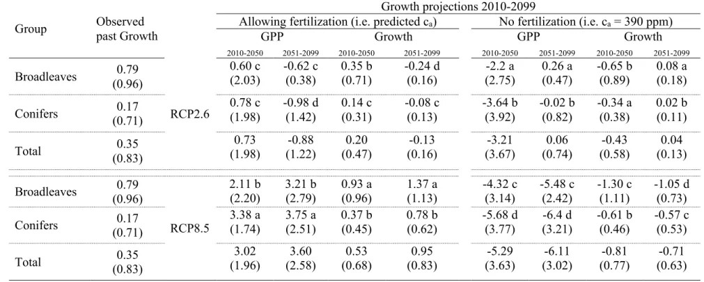
16 Group Observed past Growth
Growth projections 2010-2099
Allowing fertilization (i.e. predicted ca) No fertilization (i.e. ca = 390 ppm)
GPP Growth GPP Growth 2010-2050 2051-2099 2010-2050 2051-2099 2010-2050 2051-2099 2010-2050 2051-2099 Broadleaves 0.79 (0.96) RCP2.6 0.60 c (2.03) -0.62 c (0.38) 0.35 b (0.71) -0.24 d (0.16) -2.2 a (2.75) 0.26 a (0.47) -0.65 b (0.89) 0.08 a (0.18) Conifers (0.71) 0.17 0.78 c (1.98) -0.98 d (1.42) 0.14 c (0.31) -0.08 c (0.13) -3.64 b (3.92) -0.02 b (0.82) -0.34 a (0.38) 0.02 b (0.11) Total 0.35 (0.83) 0.73 (1.98) -0.88 (1.22) 0.20 (0.47) -0.13 (0.16) -3.21 (3.67) 0.06 (0.74) -0.43 (0.58) 0.04 (0.13) Broadleaves (0.96) 0.79 RCP8.5 2.11 b (2.20) 3.21 b (2.79) 0.93 a (0.96) 1.37 a (1.13) -4.32 c (3.14) -5.48 c (2.42) -1.30 c (1.11) -1.05 d (0.73) Conifers (0.71) 0.17 3.38 a (1.74) 3.75 a (2.51) 0.37 b (0.45) 0.78 b (0.62) -5.68 d (3.77) (3.21) -6.4 d -0.61 b (0.46) -0.57 c (0.53) Total (0.83) 0.35 (1.96) 3.02 (2.58) 3.60 (0.68) 0.53 (0.83) 0.95 (3.63) -5.29 (3.02) -6.11 (0.77) -0.81 (0.63) -0.71 331
Table 2. Growth trends as estimated by the slopes of linear regressions between growth (slopes in cm2·year-2) or GPP (slopes in g C m-2 year-2)
332
and year. Mean slopes are shown for observed past growth and for projected growth and GPP for the periods 2010-2050 and 2051-2099. 333
Standard deviations are between parentheses. One-way ANOVA differences between broadleaves and conifers (RCP2.6 and RCP85, i.e. 4 levels) 334
within columns are depicted with different letters. 335
17 336
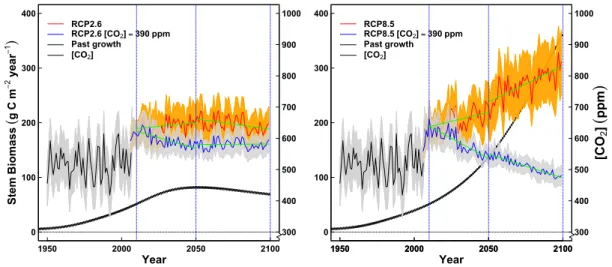
Fig. 4. Example of growth projections at one Quercus pyrenaica site (QUPY3 in
337
App.1). Trends (i.e. linear regressions between mean growth and year) for 2010-2050,
338
and 2051-2099 are shown with green lines for the ‘fertilization’ (red line) and
‘non-339
fertilization’ (blue line) scenarios. These trends correspond to the slopes reported in
340
Table 2, Fig. 5 and Fig. 6. Shaded areas behind annual mean growth values (!"; thick
341
black line is mean past growth) correspond to the confidence intervals for the mean
342
calculated as !" ± 1.96 · )*+"/√. ()*+" is the combined standard deviation of the model
343
estimates and the variability among climatic scenarios; n is sample size). ca values 344
([CO2]) corresponding to the two scenarios considered (i.e. RCP2.6, RCP8.5) are shown
345
as thin black lines.
346 347
2). GPP projections exhibited steeper trends (both positive and negative) for
348
Mediterranean conifers (all evergreen species), whereas the growth trends were steeper
349
for broadleaves (mostly deciduous) than for conifers (Table 2). An example of a model
350
simulation and how the reported trends (i.e. slopes) were calculated is depicted in Fig.
351
4. Model simulations yielded the greatest GPP and growth in more mesic sites, as
352 expected (App. 6). 353 300 400 500 600 700 800 900 1000 1950 2000 2050 2100 0 100 200 300 400 RCP2.6 RCP2.6 [CO2] = 390 ppm Past growth [CO2] 1950 2000 2050 2100 300 400 500 600 700 800 900 1000 1950 2000 2050 2100 0 100 200 300 400 RCP8.5 RCP8.5 [CO2] = 390 ppm Past growth [CO2] [C O2 ] ( p p m ) S te m B io m as s ( g C m − 2 y ea r − 1 ) Year Year
18
According to our projections forest growth would not be much altered when
354
assuming the low emission RCP2.6 scenario with predicted ca (Fig. 5). Under the ca 355
pathway from RCP2.6, which reaches the ca maximum (446 ppm) in 2051, the model
356
simulates a slight increase in growth up to 2050 followed by a slight decrease (Table 2).
357
The resulting overall trend up to 2100 depends on site conditions: most forests exhibited
358
non-significant or reduced trends under RCP2.6 for both ca scenarios (Fig. 5, 6).
359
However, for the ‘non-fertilization’ scenario, model simulations suggested significant
360
negative growth trends for some coniferous sites e.g. in Southern France and Eastern
361
Spain (Fig. 6). Therefore the results of the model mostly suggested that forests would
362
acclimate at the regional scale to the climate proposed by RCP2.6. Yet, negative local
363
impacts for some coniferous species would pop up when constraining the carbon
364
fertilization effect.
365
Climate simulations under RCP8.5 forecast a much warmer scenario with less
366
precipitation than RCP2.6 (App. 3). In response, forest growth projections under this
367
scenario showed a different picture to that described for RCP2.6. For the
‘non-368
fertilization’ scenario (i.e. constant 390 ppm) future forest growth trends would be
369
negative across all the western Mediterranean. Both conifers and broadleaves would
370
suffer huge decreases in GPP and growth concurrent with the increase in PET expected
371
under RCP8.5. These negative trends were much steeper than those for RCP2.6 (Table
372
2) and in some cases converged towards zero. In contrast, under the coherent ca pathway
373
(exponential increase in ca to 935 ppm in 2100) for RCP8.5, the model suggested that
374
plants would not only compensate the more stressing climate but also that growth and
375
GPP would be enhanced across the study region regardless of species (Fig. 6; Table 2).
376
In average RCP8.5 predicts for the studied area in average a +2ºC warmer climate
377
(with ca = 504 ppm) and a slight MAP reduction by 2050 (App. 3) compared to present
19 379
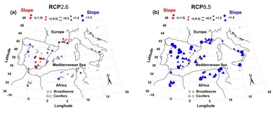
Fig. 5. Future growth simulations trends using climatic scenarios RCP2.6 (a) and RCP8.5 (b), with predicted (increasing) ca between 2010 and
380
2099. Trends are estimated as the slopes of the linear regressions between stem biomass growth and year (see Fig. 4). Symbols are scaled as a
381
function of the slope value. Red symbols correspond to negative trends whereas blue symbols to positive trends. Solid symbols correspond to
382
significant trends (α=0.05) whereas empty symbols to non-significant trends.
383 -10 -5 0 5 10 15 20 30 32 34 36 38 40 42 44 46 48 Broadleaves Conifers Europe Africa N Mediterranean Sea Longitude Lat itu de RCP2.6 <(-1.5) <(-0.5) <0.5 <1.5 >1.5 Slope Slope (a) -10 -5 0 5 10 15 20 30 32 34 36 38 40 42 44 46 48 Broadleaves Conifers Europe Africa N Mediterranean Sea Longitude Lat itu de RCP8.5 <(-1.5) <(-0.5) <0.5 <1.5 >1.5 Slope Slope (b)
20 384
Fig. 6. Future growth simulations trends between 2010 and 2099 using climatic scenarios RCP2.6 (a) and RCP8.5 (b), with constant ca = 390
385
ppm. Trends are estimated as the slopes of linear regressions between stem biomass growth and year (see Fig. 4). Symbols are scaled as a
386
function of the slope value. Red symbols correspond to negative trends whereas blue symbols to positive trends. Solid symbols correspond to
387
significant trends (α=0.05) whereas empty symbols to non-significant trends.
388 -10 -5 0 5 10 15 20 30 32 34 36 38 40 42 44 46 48 Broadleaves Conifers Europe Africa N Mediterranean Sea Longitude Lat itu de RCP2.6 <(-1.5) <(-0.5) <0.5 <1.5 >1.5 Slope Slope (a) -10 -5 0 5 10 15 20 30 32 34 36 38 40 42 44 46 48 Broadleaves Conifers Europe Africa N Mediterranean Sea Longitude Lat itu de RCP8.5 <(-1.5) <(-0.5) <0.5 <1.5 >1.5 Slope Slope (b) [CO2] = 390 ppm
21
values (i.e. +2.8ºC compared to preindustrial levels). This is over the reduction goal in
389
greenhouse emissions for COP21 (http://www.cop21paris.org/) established below +2ºC,
390
which otherwise would be achieved in RCP2.6. Simulations under RCP8.5 suggested a
391
negative impact in growth and GPP of climate unless this was compensated by an
392
exaggerated fertilization effect of eCO2. The higher the temperature, the more evident 393
and widespread this negative impact would become (Fig. 5, 6; Table 2). In contrast, 394
when allowing fertilization, the greatest positive growth trends (i.e. a greater net
395
fertilization effect) would arise after 2050 with ca levels >500 ppm (Table 2). Growth
396
trends after 2050 were steeper than those before 2050 for the ‘fertilization’ scenario
397
(mean difference 0.42, p<0.001) but not for the ‘non-fertilization’ scenario (mean
398
difference 0.09, p=0.403). This highlights the larger influence in simulated growth and
399
GPP of eCO2 (positive) compared to that of expected high temperatures (negative).
400 401
Discussion
402
Forest future in a warmer western Mediterranean region: what is the role of ca?
403
Trees can enhance productivity and modify some anatomical and physiological
404
traits (e.g. iWUE)in response to eCO2 butit is not known how they will perform under
405
future climate and ca (Medlyn & De Kauwe 2013; Duursma et al. 2016; Kelly et al. 406
2016). A positive net effect of eCO2 on trees can be hampered by the limiting effect of 407
other environmental constraints such as nitrogen (N) availability and water stress (De
408
Kauwe et al. 2013; Reichstein et al. 2013; Fernández-Martínez et al. 2014; Walker et
409
al. 2015; Kim et al. 2016). A positive feedback of eCO2, e.g. in leaf area (if a steady-410
state has not been achieved yet; Körner 2006) and NPP, has been reported under current
411
climate conditions in temperate forests where non-climatic factors such as N availability
412
were limiting (Medlyn et al. 2015; Walker et al. 2015; Kim et al. 2016). In contrast,
22
Duursma et al. (2016) did not observe any change in leaf area in response to eCO2 when
414
leaf area was limited by water availability (i.e. like in our model). Therefore, depending
415
on the most limiting factor, different ecosystems seem to express different responses to
416
eCO2 under current climatic conditions.
417
As reflected by our model during the observational period (see Gea-Izquierdo et al.
418
2015 for iWUE), the effect of recent rising ca has generally produced an enhancement in
419
iWUE but not in growth rates (e.g. Peñuelas et al. 2011; Keenan et al. 2013; Saurer et
420
al. 2014; van der Sleen et al. 2014). Furthermore, studies reporting past growth 421
enhancement within the last 150 years (e.g. at species-specific high-elevation sites) did
422
not consider ca as the main factor triggering that growth increase (Salzer et al. 2009; 423
Gea-Izquierdo & Cañellas 2014). According to our results, most Mediterranean forests
424
would mitigate the optimistic RCP2.6 scenario either with or without C-fertilization.
425
Hence, forests would mostly endure the +2°C warming limit set within the Paris’
426
Agreement (http://www.cop21paris.org/). In contrast, projections under high-emission
427
RCP8.5 would forecast big changes in forest performance. Simulations reflected a very
428
negative impact of climatic conditions under RCP8.5 and a non-fertilization scenario,
429
whereas they suggested a dominant positive effect of eCO2 at the regional scale
430
(particularly for ca > 500 ppm) when allowing fertilization even under the very limiting
431
climatic conditions of RCP8.5. The observed positive trends following a Temperature x
432
eCO2 interaction were not unexpected, because the Farquhar model ensures large direct
433
responses to eCO2 since Rubisco-limited photosynthesis responds fast to enhanced ca
434
(Reichstein et al. 2013; Friend et al. 2014; Baig et al. 2015; Walker et al. 2015; Norby
435
et al. 2016). Yet, this fertilization effect both for GPP and growth under RCP8.5 looks 436
unrealistic (Körner 2006; Friend et al. 2014; Baig et al. 2015; Kelly et al. 2016).
23
The future long-term response of forests is uncertain but we expected no positive
438
net effect of eCO2 on plant growth under very strong water-limitations (van der Molen
439
et al. 2011; Girardin et al. 2012; Baig et al. 2015). Nevertheless, this was only reflected 440
for RCP8.5 by the non-fertilization scenario. Photosynthesis is a saturating function of
441
intercellular CO2 (Kelly et al. 2016) and according to Körner (2006) saturation is
442
expected at levels similar to those of RCP8.5 in 2100 (circa 1000 ppm). Likely, the
443
model does not downregulate assimilation enough under high ca or underestimates the
444
limiting effect of other interacting factors (e.g. light, nutrients, water stress, hydraulics)
445
on e.g. maximum carboxylation. This was addressed empirically by setting a limit at
446
390 ppm but a more detailed understanding of the physiological processes in relation to
447
eCO2 would definitely help to improve model forecasts. A global negative response of
448
Mediterranean forests to intense warming unless there is an exaggerated C-fertilization
449
effect is, thus, evident in our results. Importantly, this implies negative consequences
450
for forest performance and means that a positive effect of milder winters (e.g. earlier
451
growing season or enhanced winter assimilation in evergreens) would not counteract the
452
negative effect of longer stressing summers. There is an ample debate on the actual
453
factors causing tree death, but it seems that a combination of interrelated C-related
454
traits, hydraulically-related features and climate-related impacts of biotic agents should
455
govern the forest decline and mortality processes (Sala et al. 2012; McDowell et al.
456
2013; Aguadé et al. 2015; Anderegg et al. 2015). Regardless of the final causal factor/s,
457
steep negative growth trends like those under RCP8.5 and no-fertilization strongly 458
suggest changes in stand dynamics and composition and ultimately enhanced mortality 459
at some sites (Bigler et al. 2006; van der Molen et al. 2011; Gea-Izquierdo et al. 2014). 460
461
Forest growth projections under climate change and eCO2: utilities and uncertainties
24 Models need continuous refinement to achieve robustness, reliability and realism 463
(Prentice et al. 2015). Forecasts of tree growth are a valuable tool to understand forest
464
performance under climate change but there are many sources of uncertainty within
465
model performance and data-assimilation that need discussion (Friend et al. 2014).
466
Caveats in models include: (i) current knowledge of the physiological processes; (ii)
467
model implementation and parameterization (including scale-dependent constraints);
468
(iii) uncertainty of model outputs outside the calibration range (Pappas et al. 2013;
469
Prentice et al. 2015). Additionally, changes in plasticity of functional traits and plant 470
acclimation processes can bias model projections (Muller et al. 2011). We assumed
471
uniformitarianism (i.e. temporal invariance of the modeled relationships) in model
472
projections but it could be that threshold related responses arise after the calibration
473
boundaries are surpassed. In this sense (iii) is minimized by explicitly modeling
474
processes but not eliminated as a result of (i) and (ii). Despite inherent limitations in
475
models and observational data (Babst et al. 2014), by using data-assimilation we
476
maximized the likelihood of getting unbiased past long-term trends to increase
477
reliability of growth projections (Peng et al. 2011; Medlyn et al. 2015). Forest
478
productivity was analyzed assuming present steady-state stand conditions (e.g. 479
composition, leaf area, root mass) constrained by water stress (Körner 2006). This could 480
bias the analysis of forest dynamics (Körner 2003; Friend et al. 2014; Pappas et al. 481
2015), particularly for mixed stands (Pappas et al. 2013). However, our aim was to
482
analyze performance of the present stands under future environmental conditions, with 483
emphasis on species long-term trends. Changes in inter-species dynamics are away from 484
the scope of our analysis and need to be studied complementary. 485
The model does not include nutrient dynamics but focuses on the water and carbon
486
cycles and the effect of water stress at different functional levels. This is because
25
nutrient availability is generally considered secondary in Mediterranean ecosystems
488
compared to water stress, which in addition is expected to increase in the future (Giorgi
489
& Lionello 2008; García-Ruiz et al. 2011; IPCC 2014). Thus, the limiting effect of 490
factors such as availability of N, P, or hydraulic constraints could invalidate a C 491
fertilization effect on net growth under eCO2 (Körner 2006; Norby et al. 2010; Fatichi
492
et al. 2014; Fernández et al. 2014; Friend et al. 2014; Baig et al. 2015). Our model is
493
simpler than ecosystem models including nutrient and stand dynamics (e.g. Reichstein
494
et al. 2013; Walker et al. 2015). However, our scale is finer (stand, species-specific 495
compared to PFTs) and, most important, it is driven by actual growth data to ensure
496
unbiased estimation of short- and long-term trends. Other factors such as differences in
497
carry-over effects between conifers and broadleaves, changes in species composition
498
and demography, competition and tree-related traits such as ontogeny and size, partly
499
modulate the forest response to climate (van der Molen et al. 2011). However, l
ong-500
term stand productivity seems to change slightly under moderate disturbances such as
501
those produced by silvicultural treatments or insect infestation (Vesala et al. 2005;
502
Amiro et al. 2010). Therefore, we believe that climate effects are dominant and the
503
reported long-term trends are robust in relation to variability within these other factors,
504
which would affect mostly in the short-term. The model fit reported was in the range of
505
that in similar studies (Misson 2004; Li et al. 2014; Gea-Izquierdo et al. 2015; Girardin
506
et al. 2016). Different goodness-of-fit at different sites could result on differences in 507
model performance. However, in App. 7A we show how variability in R2 did not
508
influence the estimated trends (future projections). Particularly, when the trees exhibited
509
long-term trends in the past (observational period), these showed a very high agreement
510
with the modeled growth trends (App. 7B; Table 1). As mentioned, the robustness of
511
our approach relies on the spatial (regional) scale where the model was applied, which
26
expands model implementation at a broader scale than that where it was previously
513
applied (Misson et al. 2004; Gaucherel et al. 2008; Gea-Izquierdo et al. 2015).
514
Model simulations can be improved by better addressing the influence of CO2 on 515
variability of different plant traits (Kattge et al. 2011; Atkin et al. 2015; Pappas et al.
516
2016). Leaf photosynthesis is negatively affected by drought through several
517
mechanisms including changes in stomatal and mesophyll conductance or reductions in
518
biochemical efficiency (Flexas et al. 2005). Both photosynthesis and stomatal
519
conductance were modeled as direct functions of CO2. However, warming and
520
increasing water stress in relation to eCO2 could differently affect autotrophic
521
respiration and photosynthetic capacity, or enhance photorespiration more than
522
photosynthesis (Baig et al. 2015; Girardin et al. 2016; Rowland et al. 2015; Varone &
523
Gratani 2015). Our model takes into account the short-term acclimation of leaf
524
photosynthesis and stomatal conductance to CO2, while respiration is set as a function
525
of temperature and GPP (Gea-Izquierdo et al. 2015). Different sources of interspecific
526
variability under eCO2 in autotrophic respiration not explained by models (Atkin et al.
527
2015) or other factors such as species-specific variability in Jmax/Vcmax could partly
528
impair our results. Trees modify other traits such as leaf area and sapwood area to
529
withstand xericity (Breda et al. 2006; Martin-StPaul et al. 2013; Duursma et al. 2016;
530
Kelly et al. 2016). In our model, intra-annual, inter-annual and long-term structural
531
acclimation of leaf area and allocation rules rely on climate and SWC but not on CO2.
532
Thus, addressing the influence of CO2 on leaf area dynamics by setting SLA and
533
allocation rules also as functions of CO2 could also help to better assess whether the 534
reported fertilization effect is unrealistic (Duursma et al. 2016; Medlyn et al. 2015).
535
In summary, modeled forest growth reflected the observed absence of an overall net 536
positive effect of enhanced ca under increased temperatures (i.e. PET) in the recent past.
27 According to model projections, western Mediterranean forests would mostly mitigate 538
the negative effect of a climate remaining below the maximum warming levels (+2ºC) 539
agreed in COP21 (i.e. scenario RCP2.6) but the situation would be very different above 540
those levels (as represented by RCP8.5). Our results suggest that fertilization could 541
override the negative effect of stressing climatic conditions under high-emission 542
RCP8.5 but this fertilization effect of eCO2 looks unrealistic according to the literature,
543
being most likely a result of miss-performance of models way above the calibration ca
544
levels. Consequently, simulations precluding fertilization under high-emission scenarios 545
show very negative forest performance at the regional scale in the future for both 546
conifers and broadleaves. Our results suggest that western Mediterranean forests would 547
not resist the stressing conditions of a much warmer climate unless species exhibited an 548
exaggerated C fertilization effect. It is necessary to include ca variability in forest
549
models but it is not enough. We still need a better understanding of the physiological 550
processes governing the capacity of acclimation of different plant traits (e.g. Vcmax) to
551
the interaction between water stress, eCO2 and nutrient availability. In this sense, our 552
simulations precluding a fertilization effect seems more realistic than those allowing 553
fertilization under ca levels way above those used to calibrate models. Our study
554
provides a comprehensive data-driven analysis of the likely performance of western
555
Mediterranean forests under predicted climate change and ca. Yet model performance
556
still needs to be refined under high ca as expected in the future.
557 558
Acknowledgements
559
This study was funded by project AGL2014-61175-JIN of the Spanish Ministry of
560
Economy and Competitiveness and the Labex OT-Med (n° ANR-11-LABEX-0061)
561
from the «Investissements d’Avenir» program of the French National Research Agency
28
through the A*MIDEX project (n° ANR-11-IDEX-0001-02). The climate simulations
563
have been extracted from the CMIP5 site (
https://esgf-index1.ceda.ac.uk/projects/esgf-564
ceda/) and processed with the help of Romain Suarez.
565 566
References
567
Aguadé D, Poyatos R, Gómez M, Oliva J, Martínez-Vilalta J (2015) The role of
568
defoliation and root rot pathogen infection in driving the mode of drought-related
569
physiological decline in Scots pine (Pinus sylvestris L.). Tree Physiology, 35, 229–
570
242.
571
Allen RG, Pereira LS, Raes D, Smith M (1998) Crop Evapotranspiration – Guidelines
572
for Computing Crop Water Requirements, FAO Irrigation and Drainage Paper 56,
573
FAO, 1998, ISBN 92-5-104219-5.
574
Amiro BD, Barr AG, Barr JG et al. (2010) Ecosystem carbon dioxide fluxes after
575
disturbance in forests of North America. Journal of Geophysical Research:
576
Biogeosciences, 115, G00K02, doi:10.1029/2010JG001390.
577
Anderegg WRL, Schwalm C, Biondi F et al. (2015) Pervasive drought legacies in forest 578
ecosystems and their implications for carbon cycle models. Science, 1, 528–532. 579
Atkin OK, Bloomfield KJ, Reich PB et al. (2015) Global variability in leaf respiration 580
in relation to climate, plant functional types and leaf traits. New Phytologist, 206, 581
614–636. 582
Babst F, Alexander MR, Szejner P et al. (2014) A tree-ring perspective on the terrestrial 583
carbon cycle. Oecologia, 176, 307–322. 584
Baig S, Medlyn BE, Mercado LM, Zaehle S (2015) Does the growth response of woody 585
plants to elevated CO2 increase with temperature? A model-oriented meta-analysis.
586
Global Change Biology, 21, 4303–4319. 587
29 Baldocchi DD, Ma SY, Rambal S et al. (2010) On the differential advantages of
588
evergreenness and deciduousness in mediterranean oak woodlands: a flux 589
perspective. Ecological Applications, 20, 1583–1597. 590
Battipaglia G, Saurer M, Cherubini P, Calfapietra C, McCarthy HR, Norby RJ, Cotrufo
591
MF (2013) Elevated CO2 increases tree-level intrinsic water use efficiency:
592
insights from carbon and oxygen isotope analyses in tree rings across three forest
593
FACE sites. New Phytologyst, 197, 544-554.
594
Bigler C, Braker OU, Bugmann H, Dobbertin M, Rigling A (2006) Drought as an 595
inciting mortality factor in Scots pine stands of the Valais, Switzerland. 596
Ecosystems, 9, 330–343. 597
Breda N, Huc R, Granier A, Dreyer E (2006) Temperate forest trees and stands under 598
severe drought: a review of ecophysiological responses, adaptation processes and 599
long-term consequences. Annals of Forest Science, 63, 625–644. 600
De Kauwe MG, Medlyn BE, Zaehle S et al. (2013) Forest water use and water use 601
efficiency at elevated CO2: a model-data intercomparison at two contrasting
602
temperate forest FACE sites. Global Change Biology, 19, 1759–1779. 603
Duursma RA, Gimeno TE, Boer MM, Crous KY, Tjoelker MG, Ellsworth DS (2016) 604
Canopy leaf area of a mature evergreen Eucalyptus woodland does not respond to 605
elevated atmospheric [CO2] but tracks water availability. Global Change Biology,
606
22, 1666-1676. 607
Falge E, Baldocchi D, Tenhunen J et al. (2002) Seasonality of ecosystem respiration 608
and gross primary production as derived from FLUXNET measurements. 609
Agricultural and Forest Meteorology, 113, 53–74. 610
Farquhar GD, von Caemmerer S, Berry JA (1980) A biochemical model of 611
photosynthetic CO2 assimilation in leaves of C3 species, Planta, 149, 78–90.
30 Fatichi S, Leuzinger S, Körner C (2014) Moving beyond photosynthesis : from carbon 613
source to sink-driven vegetation modeling. New Phytologist, 201, 1086–1095. 614
Fatichi S, Pappas C, Ivanov VY (2015) Modeling plant-water interactions: an 615
ecohydrological overview from the cell to the global scale. Wiley Interdisciplinary 616
Reviews Water 3, 327–368. 617
Fernández-Martínez M, Vicca S, Janssens IA et al. (2014) Nutrient availability as the 618
key regulator of global forest carbon balance. Nature Climate Change, 4, 471–476. 619
Flexas J, Bota J, Galmes J, Medrano H, Ribas-Carbo M (2006) Keeping a positive 620
carbon balance under adverse conditions: responses of photosynthesis and 621
respiration to water stress. Physiologia Plantarum, 127, 343–352. 622
Friend AD, Lucht W, Rademacher TT et al. (2014) Carbon residence time dominates 623
uncertainty in terrestrial vegetation responses to future climate and atmospheric 624
CO2. Proceedings of the Natural Academy of Sciences of the United States of
625
America, 111, 3280–5. 626
Fritts HC (1976) Tree Rings and Climate. Blackburn Press, p. 567. 627
García-Ruiz JM, Ignacio Lopez-Moreno J, Vicente-Serrano SM, Lasanta-Martinez T, 628
Begueria S (2011) Mediterranean water resources in a global change scenario. 629
Earth-Science Reviews, 105, 121–139. 630
Gaucherel C, Guiot J, Misson L (2008) Evolution of the potential distribution area of 631
french mediterranean forests under global warming. Biogeosciences, 5, 1493– 632
1504. 633
Gea-Izquierdo G, Cañellas I. (2014) Contrasting instability in growth trends of
634
Mediterranean oaks at opposite distributional limits. Ecosystems, 17, 228-241.
31 Gea-Izquierdo G, Viguera B, Cabrera M, Cañellas I (2014) Drought induced decline 636
could portend widespread pine mortality at the xeric ecotone in managed 637
mediterranean pine-oak woodlands. Forest Ecology and Management, 320, 70–82. 638
Gea-Izquierdo G, Guibal F, Joffre R, Ourcival J-M, Simioni G, Guiot J. (2015) 639
Modelling the climatic drivers determining photosynthesis and carbon allocation in 640
evergreen Mediterranean forests using multiproxy long time series. 641
Biogeosciences, 12, 3695-3712. 642
Giorgi F, Lionello P (2008) Climate change projections for the Mediterranean region. 643
Global and Planetary Change, 63, 90–104. 644
Girardin MP, Bernier PY, Raulier F, Tardif JC, Conciatori F, Guo XJ (2012) Testing for 645
a CO2 fertilization effect on growth of Canadian boreal forests. Journal of
646
Geophysical Research-Biogeosciences, 116, G01012, doi:10.1029/2010JG001287. 647
Girardin MP, Hogg EH, Bernier PY, Kurz WA, Guo XJ, Cyr G (2016) Negative 648
impacts of high temperatures on growth of black spruce forests intensify with the 649
anticipated climate warming. Global Change Biology, 22, 627–643. 650
Guiot J, Boucher E, Gea-Izquierdo G (2014) Process models and model-data fusion in 651
dendroecology. Frontiers in Ecology and Evolution, 2, 1–12. 652
Herrera S, Gutierrez JM, Ancell R, Pons MR, Frias MD, Fernandez J (2012) 653
Development and Analysis of a 50 year high-resolution daily gridded precipitation 654
dataset over Spain (Spain02). International Journal of Climatology, 32, 74-85. 655
IPCC (2014) Climate Change 2014: Synthesis Report. Contribution of Working Groups 656
I, II and III to the Fifth Assessment Report of the Intergovernmental Panel on 657
Climate Change [Core Writing Team, R.K. Pachauri and L.A. Meyer (eds.)]. 658
IPCC, Geneva, Switzerland, 151 pp. 659