HAL Id: hal-00296404
https://hal.archives-ouvertes.fr/hal-00296404
Submitted on 4 Jan 2008
HAL is a multi-disciplinary open access
archive for the deposit and dissemination of
sci-entific research documents, whether they are
pub-lished or not. The documents may come from
teaching and research institutions in France or
abroad, or from public or private research centers.
L’archive ouverte pluridisciplinaire HAL, est
destinée au dépôt et à la diffusion de documents
scientifiques de niveau recherche, publiés ou non,
émanant des établissements d’enseignement et de
recherche français ou étrangers, des laboratoires
publics ou privés.
condensation, evaporation and rain in warm cumulus
cloud
O. Altaratz, I. Koren, T. Reisin, A. Kostinski, G. Feingold, Z. Levin, Y. Yin
To cite this version:
O. Altaratz, I. Koren, T. Reisin, A. Kostinski, G. Feingold, et al.. Aerosols’ influence on the interplay
between condensation, evaporation and rain in warm cumulus cloud. Atmospheric Chemistry and
Physics, European Geosciences Union, 2008, 8 (1), pp.15-24. �hal-00296404�
Atmos. Chem. Phys., 8, 15–24, 2008 www.atmos-chem-phys.net/8/15/2008/ © Author(s) 2008. This work is licensed under a Creative Commons License.
Atmospheric
Chemistry
and Physics
Aerosols’ influence on the interplay between condensation,
evaporation and rain in warm cumulus cloud
O. Altaratz1, I. Koren1, T. Reisin2, A. Kostinski3, G. Feingold4, Z. Levin5, and Y. Yin6
1Department of Environmental Sciences, Weizmann Institute, Rehovot, Israel 2Soreq Nuclear Research Center, Yavne, Israel
3Department of Physics, Michigan Technological University, Houghton, Michigan, USA 4NOAA Earth System Research Laboratory, Boulder, Colorado, USA
5Department of Geophysics and Planetary Sciences, Tel Aviv University, Tel Aviv, Israel
6Department of Applied Meteorology, Nanjing University Information Science & Technology, Nanjing, China
Received: 23 August 2007 – Published in Atmos. Chem. Phys. Discuss.: 29 August 2007 Revised: 13 November 2007 – Accepted: 5 December 2007 – Published: 4 January 2008
Abstract. A numerical cloud model is used to study the
influence of aerosol on the microphysics and dynamics of moderate-sized, coastal, convective clouds that develop un-der the same meteorological conditions. The results show that polluted convective clouds start their precipitation later and precipitate less than clean clouds but produce larger rain drops. The evaporation process is more significant at the margins of the polluted clouds (compared to the clean cloud) due to a higher drop surface area to volume ratio and it is mostly from small drops. It was found that the formation of larger raindrops in the polluted cloud is due to a more effi-cient collection process.
1 Introduction
The effect of aerosol on clouds and precipitation is still one of the largest uncertain factors in the fields of cloud physics and climate change. It is clear that a higher aerosol loading leads to more cloud condescension nuclei (CCN) and possi-bly more ice nuclei and therefore to different size distribu-tions of the water and ice particles. However the derived re-sults on the cloud lifetimes, structures and precipitation pat-terns are harder to predict due to the interplay between com-plex feedbacks (e.g., Xue and Feingold, 2006; Jiang et al., 2006).
Numerous studies have addressed the effect of aerosol on marine stratocumulus clouds, due to their key role in the global radiative energy. Marine stratocumuli, bounded by strong marine boundary layer inversion, have relatively
Correspondence to: O. Altaratz
uniform-layered structure that facilitates comparison be-tween clean and polluted clouds. Marine stratocumulus clouds that form in polluted environments were hypothesized to contain more but smaller droplets and to have a higher re-flectivity (Twomey, 1974, 1977). Albrecht (1989) suggested that cloud liquid water path (LWP), fractional cloudiness and cloud lifetime of stratocumulus will increase through aerosol-induced precipitation suppression. A few in situ measurements conducted in ship tracks (Radke et al., 1989; King et al., 1993; Ferek et al., 1998, 2000) observed a de-crease in drizzle-size drops in the tracks. But in contrast to Albrecht’s theory, observational studies of aerosol effects on liquid water path (LWP) of stratocumulus clouds have shown that it can increase, decrease or remain the same un-der the influence of increased concentration of aerosol parti-cles (Platnick et al., 2001; Coakley and Walsh, 2002; Han et al., 2002). Ackerman et al. (2004) simulated stratocumulus clouds with a fluid dynamic model (including detailed treat-ment of cloud microphysics and radiative transfer) to study this controversy. They concluded that the response of the cloud LWP to changes in aerosol loading is influenced by the humidity profile above the inversion and is determined by a competition between moistening from decreased sur-face precipitation and drying from increased entrainment of overlying air. Their results also showed a decrease in the precipitation at the ground from polluted clouds.
Unlike stratiform clouds, convective clouds, controlled more by local instability, have larger variability and are more difficult to analyze by remote sensing methods. Therefore, detailed microphysical numerical models can serve as a valu-able tool to understand the effects of aerosol on the complex feedbacks between cloud microphysical and dynamical pro-cesses.
This study focuses on the processes taking place in a moderate-size warm, cumulus cloud, without active ice pro-cesses.
Aerosol effects on shallow (small) cumulus clouds have been studied in recent years mostly by numerical models. Satellite data limited by the pixel sizes will be biased to-ward larger clouds with stronger spectral and spatial signa-ture. Recent numerical experiments that focused on the ef-fect of aerosol on LWC, dimensions and lifetime of warm cu-mulus clouds have shown different results from deep clouds. Xue and Feingold (2006) studied the effects of aerosol on warm trade-wind cumulus clouds using large eddy simula-tions (LES) with size-resolved cloud microphysics. They showed that an increase in aerosol concentration led to a re-duction in cloud fraction, cloud size, cloud top-height and depth, and precipitation on the ground. This study exam-ined the evolution of a field of cumulus clouds and noted that the dynamical variability associated with the cloud field may sometimes mask the aerosol effect on some cloud proper-ties. They concluded that the complex responses of clouds to aerosol are determined by competing effects of precipitation and droplet evaporation associated with entrainment. Jiang and Feingold (2006) used a different LES model to show the effect of aerosol on warm convective clouds over land. Their results showed that in the absence of aerosol radiative effects, an increase in aerosol loading results in a reduction in precipitation at the ground but no statistically significant changes in LWP, cloud fraction and depth. On the other hand including the aerosol radiative effects resulted in a reduction in LWP, cloud fraction and depth, primarily due to the re-duction in surface forcing associated with absorbing aerosol. Jiang et al. (2006) who studied the influence of aerosol on the lifetime of shallow clouds showed that an evaporation-entrainment feedback tends to dilute polluted clouds more than clean clouds. This process is the cause of the reduc-tion or no change in lifetime of polluted clouds. LES results indicated no significant change in cloud lifetime as a result of aerosol whereas single cloud model simulations showed reductions in cloud lifetime. Xue et al. (2007) studied shal-low cumulus clouds under stratocumulus (using LES) and showed that cloud fraction increased with increasing aerosol only for relatively low values of aerosol concentrations (up to 100 cm−3in their case). A further increase in aerosol particle
concentration results in reduced cloud fraction. They sug-gested that opposing effects of aerosol induced suppression of precipitation and aerosol induced enhancement of evapo-ration are responsible for this non monotonic behavior.
These studies imply that in small clouds, evaporation plays a key role in determining cloud properties in response to an increase in aerosol loading.
The aim of this study is to investigate the role of aerosol in warm convective clouds, from the drop (micro) scale to the cloud property (macro) scale, by affecting the interplay between the processes of: diffusional growth, evaporation of drops, and growth by collision-coalescence. All these
pro-cesses start at the small scale of aerosol and drops but in-fluence and create the large scale of cloud characteristics. We examine the effects of aerosol on the size distribution of cloud droplets and rain drops and subsequently on cloud properties and precipitation patterns.
2 The model
We used the Tel Aviv University axisymmetric non-hydrostatic numerical cloud model (TAU-CM) with detailed treatment of cloud microphysics (Tzivion et al., 1994; Reisin et al., 1996). The warm microphysical processes included are nucleation of CCN, condensation and evaporation, collision-coalescence, binary breakup, and sedimentation. The micro-physical processes are formulated and solved using a multi-moment bin method (Tzivion et al., 1987).
The drop activation scheme is based on the supersatura-tion and critical diameter determined by the Kohler curves (Pruppacher and Klett, 1997). Calculations of the critical diameter for aerosol activation were done by assuming that CCN are composed of pure sea-salt (NaCl). Since cloud con-densation nuclei begin to grow by absorption of water vapor long before they enter the cloud, these wetted particles pro-vide the initial sizes for subsequent condensational growth (Kogan, 1991). Following this approach and based on Yin et al. (2000, 2002) we assumed that the initial droplet size formed on CCN with radii smaller than 0.12 µm is equal to the equilibrium radius at 100% RH. For larger CCN, the initial radii are smaller than their equilibrium radii at 100% RH by a factor proportional to the droplet radius. Once the droplets reach their critical size or the size calculated based on Kogan (1991) and Yin et al. (2000) they are placed in the appropriate bin for subsequent growth.
There are no radiation processes in the model.
3 Results
3.1 Model setup
The aerosol spectrum is approximated by superimposing three lognormal distributions with parameters representing a maritime air mass (Jaenicke, 1988):
dN (r) d(log r) = 3 X i=1 ni √ 2π log σi exp ( − (log r/Ri)2 2(log σi)2 ) (1)
Table 1 present the parameters of the distribution. The total number concentration of aerosol is 295 cm−3. In this study
we assume that all the aerosols are CCN.
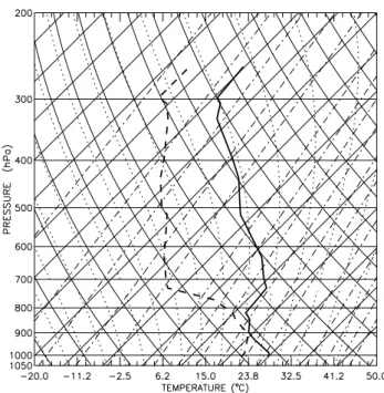
The simulations were initialized with a homogeneous base-state environment of an Israeli autumn day, based on 1 October 2006, 12Z sounding of temperature and moisture from the Bet Dagan meteorological station (without winds). To better approximate conditions at the coast that enhance
O. Altaratz et al.: Aerosols’ influence on warm cumulus cloud 17
Table 1. Parameters for the aerosol particle distribution: ni = total number of aerosol particles per cubic centimeter of air, Ri = geo-metric mean aerosol particle radius in mm, σi= standard deviation in mode i.
Mode i ni(cm−3) Ri(µm) log σi
1 133 0.039 0.657
2 66.6 0.133 0.210
3 3.06 0.29 0.396
convective development, some modifications to the sound-ing were necessary. These modifications included addition of moisture near the surface, a temperature decrease near the surface, and an increase in inversion height (Fig. 1).
The grid resolution was set to 100 m in both radial and vertical directions. The domain was 5100 m in the radial di-rection and 6100 m in the vertical. Convection was initiated by introducing a warm bubble in a small region at the lower boundary of the grid at the domain origin, for one time step. The bubble was warmer by 2◦C from the environment. The
time step of the computation was 2 s and the total simulation time was 90 min. Open boundary conditions were assumed.
Three simulations were performed, for different levels of pollution. The pollution aerosols were added to the back-ground (clean) aerosol distribution in one bin corresponding to a size of 0.3 microns. Cloud 1 represents the clean case (only background aerosols), cloud 2 represents a cloud with 800 cm−3polluted particles and cloud 3 represents a cloud
with 1600 cm−3polluted particles.
3.2 Simulations results
3.2.1 Condensation and evaporation interplay
In all the simulations the clouds start to form after ∼10 min of simulation. The appearance of the maximum vertical depth of these clouds is about 1300 m. The maximal value of the updraft in the cloud is delayed as the cloud is more polluted, in accord to a delay in rainfall initiation. The max-imal values are 4.3 m s−1 for the clean cloud (at 34 min of
simulation), 4.5 m s−1for cloud 2 (at 44 min) and 4.4 m s−1
for the most polluted cloud (at 48 min).
The vertical changes in drop mass and number and the rel-ative importance of the condensation and evaporation pro-cesses are examined for the cores and margins of the clouds, for the different pollution levels. Note that use of the term “core” is not meant to suggest an adiabatic cloud core, but simply the region of the cloud close to its center. Figures 2–3 and 5 show the vertical profiles of drop concentration, drop mass mixing ratio and net evaporated/condensed mass mix-ing ratio at the cloud center and 500 m from cloud center for three stages of cloud development. The point at 500 m from cloud center was chosen to represent cloud margins since it is
Fig. 1. Vertical profiles of temperature and dew point based on 1
October 2006 12Z from Bet Dagan meteorological station, Israel.
far enough from cloud center and it is exposed to entrainment with the drier air, outside the cloud.
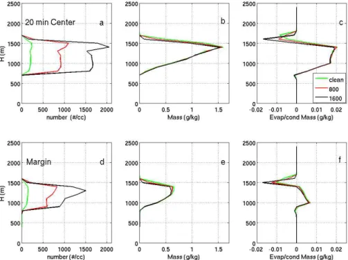
Figure 2 corresponds to the developing stage of the clouds, at 20 min of simulation. At this stage there is still no precip-itation on the ground for any of the clouds. Cloud top height is 1700 m for the clean cloud and 1600 m for the polluted clouds. The top of the clouds are defined as the highest grid point with a mass mixing ratio greater than 0.01 g kg−1.
The differences in the drop number concentrations are eas-ily recognized at all heights for the three clouds. As ex-pected, the most polluted cloud has the highest drop con-centration at cloud center. The maximum drop concentra-tion for the clean cloud is 239 cm−3(at 1500 m height), for
cloud 2 it is 1111 cm−3(at 1500 m) and for the most polluted
cloud 2053 cm−3, at 1400 m. The evaporation at the top of
the clouds is shown both at the cloud centers (Fig. 2c) and cloud margins (Fig. 2f) and is commensurate with the pollu-tion loading. The enhanced evaporapollu-tion is promoted by the smaller size of the drops near the polluted cloud top; due to higher surface to volume ratio there is an increase in the effi-ciency of the evaporation process (Xue and Feingold, 2006; Jiang and Feingold, 2006). It is also shown that due to the en-hanced evaporation, there is less liquid water mass at the top of the polluted clouds (Fig. 2b) and their top height is lower (Xue and Feingold, 2006). The downdraft values at clouds top at 22 min of simulation are −0.6 m s−1for the most
pol-luted cloud and −0.2 m s−1 for the clean cloud, indicating
higher evaporative cooling in the polluted cloud at this stage. Another evidence for that is the thermal gradient at cloud top height, between cloud core and margins, which is −0.4◦in
Fig. 2. The vertical profiles of drop concentration (left boxes), drops mass (central boxes) and net evaporated and condensed mass (during a
time step), at 20 min of simulation, for the centers (upper panel) and margins (500 m from cloud center) of the three clouds. Cloud 1 (clean) – green curve, cloud 2 (800 cm−3) – red curve, cloud 3 (1600 cm−3) – black curve.
the clean case and −0.8◦in the most polluted one. Net
evap-oration rates can be also seen at the base of the clouds where the droplets are exposed to dry air from below but differences are negligible because of the small amounts of water at cloud base.
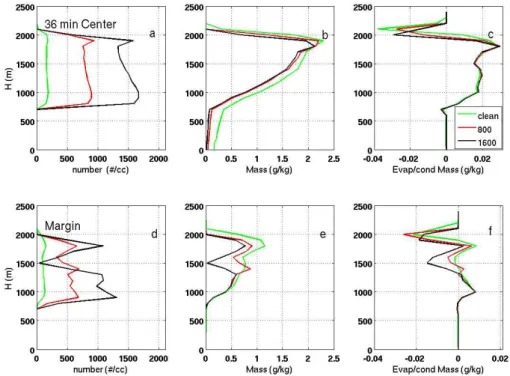
By 36 min (Fig. 3) precipitation reaches the ground in all three case; the rain rates below cloud center are 5.8, 1.7 and 0.8 mm h−1for cloud 1, 2 and 3, respectively. At this stage,
cloud top-height is almost similar for all clouds.
The vertical profiles at clouds margins present a different picture from those at the cloud cores. The most significant difference is for the polluted clouds. While in the cores of the polluted clouds there is net condensation of water mass, at the margins there is a net evaporation over the upper half of the cloud volume. At the margin of the most polluted cloud most of the region above 1400 m is influenced by evapora-tion. This is clearly demonstrated by the lower drop con-centration and mass profiles at the periphery of the polluted clouds. There is a reduction in the value of the drop con-centration and mass in the region between 1400–1800 m, in-dicating that there are regions in the polluted cloud margins which contain fewer drops (both in mass and number) than in the corresponding locations in the clean cloud. Due to that there are differences in clouds width corresponding to the pollution loading. At this stage the mean width of the clean cloud is 404 m, for cloud 2 it is 357 m and for the most polluted cloud it is 347 m (the clouds boundaries are
defined by the grid points with a mass mixing ratio greater than 0.01 g kg−1). Examination of the drop size distribution
at this stage reveals that there are two separate modes in the distribution (as presented later in Fig. 8). Checking the rel-ative importance of those two modes in the evaporation pro-cess near the most polluted cloud edge reveals that 99% of the mass evaporated between 1400–2000 m is from the small drops (with a diameter <100 microns). This evaporation pro-cess exists also in the clean case but it is more significant as the pollution level increases, driven by the higher num-ber of small size drops and higher surface area to volume ratio. Near the top of the cloud, at this stage, evaporation rates are higher in the clean case (see Fig. 3c), due to larger mass available for evaporation at this level. Higher evapora-tion rates at the beginning of the cloud growth in the most polluted cloud (Fig. 2c) caused a significant reduction in the drop mass which can be evaporated at this level.
A consequence of enhanced evaporation process, at the polluted clouds margins, is the generation of stronger hori-zontal winds. We expect to find stronger downdrafts in the polluted clouds margins, due to higher evaporative cooling (Xue and Feingold, 2006). These downdrafts will cause an enhancement of the horizontal winds and therefore enhance-ment of the entrainenhance-ment. Figure 4 presents the vertical pro-files of the horizontal wind velocities, 600 m from cloud cen-ter, for the three clouds, at 36 min of simulation. The stronger radial winds between 1200–1700 m for the most polluted
O. Altaratz et al.: Aerosols’ influence on warm cumulus cloud 19
Fig. 3. As in Fig. 3 but for 36 min of simulation.
cloud, indicate an enhanced mixing between the outer, drier air and the cloud. These results are consistent with those pre-sented by Xue and Feingold (2006) and Jiang et al. (2006) who argued that the smaller drops associated with polluted clouds evaporate more readily. They hypothesized that the enhanced evaporation is responsible for a stronger horizon-tal buoyancy gradient which increases the vertical circulation around the core of the cloud, and increases dilution via en-trainment (Zhao and Austin, 2005). The thermal gradient between clouds’ core and boundary can represent the hori-zontal buoyancy gradient. It was checked for a horihori-zontal plan at 1300 m height (the central part of the cloud) for the three clouds and the results show that during all stages in the clouds lifetime, the clean cloud has a smaller thermal gradi-ent than the polluted clouds.
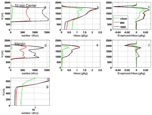
At 52 min of simulation (Fig. 5), cloud top is at 2100 m for all clouds. At this stage in the clean cloud there is less liquid water mass, in the upper region of the cloud in the central part and along most of the margin, compared to the polluted clouds (in contrary to the previous stage, presented in Fig. 3). The higher rain rate of the clean cloud has caused a redistribution of water to lower altitudes (Fig. 5b). At the periphery of the clean cloud there is mostly evaporation at this stage (Fig. 5f); while in the more polluted cases there is still condensation of water at certain levels, suggesting that they are still actively growing. The decaying stage of the clean cloud starts earlier than the polluted clouds because of the enhanced precipitation which cools the surface, stabilizes the atmosphere, and suppresses convection. Yet, the mean width of the clean cloud at this stage is still larger than those
Fig. 4. The vertical profiles of horizontal wind velocity, at 36 min of
simulation, for the margins (600 m from cloud center) of the three clouds. Cloud 1 (clean) – green curve, cloud 2 (800 cm−3) – red curve, cloud 3 (1600 cm−3) – black curve.
of the polluted ones (431 m for the clean cloud and 354 m for the most polluted cloud).
3.2.2 Effects of pollution on rain characteristics
All the clouds precipitated during their life cycle. The rain rates below cloud center as a function of time are shown in Fig 6. Ground precipitation (at intensity >0.01 mm h−1)
started at about 29 min of simulation for the clean cloud, at 32 min for cloud 2 and at 33 min for the most polluted cloud. The precipitation volume at ground level after 90 min
Fig. 5. As in Fig. 3 but for 52 min of simulation. Box g is zoomed-in vertical profiles of drop concentration, below the centers of the three
clouds bases.
.
Fig. 6. The rain rate (mm/h) as a function of time for the 3 clouds.
Cloud 1 (clean) – green curve, cloud 2 (800 cm−3) – red curve, cloud 3 (1600 cm−3) – black curve.
of simulation was 1844 m3 for the clean cloud, 832 m3 for cloud 2 and 520 m3 for the most polluted cloud. As ex-pected, (e.g. Yin et al., 2000; Khain et al., 2005; Teller and Levin, 2006) rain initiation is delayed, lasts longer and the total amount decreases as the cloud becomes more polluted. The time evolution of the rain efficiency (rainfall divided by total amount of condensed water) is similar in trend to the rain rate (Fig. 6). It has the highest values for the clean cloud case during most of the simulation (with a peak value of 7%)
it is lower for cloud 2 (with a peak value of 1.5%) and for the most polluted it is has the lowest values with a peak value of 1.3%.
Next we examine the rain properties below the cloud as influenced by the amount of pollution. Special focus is devoted to analysis of the interplay between evapora-tion/condensation and collision-coalescence processes for the different pollution levels.
Figure 7 shows the mean drop radius for the clean and the most polluted cloud, for the cloud cores and margins, at 52 min of simulation. In general it can be seen that the mean radius of the raindrops below cloud base (below ∼800 m) is much larger than the mean radius of the drops in the cloud. This is because inclusion of the small non-precipitating cloud drops reduces the calculated mean size. Even if they fall be-low cloud base, they are the first to evaporate in the sub-saturated environment. The evaporation process just below cloud base can be recognized as a peak in the vertical evap-oration/condensation mass vertical profile in Fig. 5c. Note that there is evidence of greater sub-cloud evaporation in the clean case primarily because more water is available for evaporation over a deeper layer than in the more polluted cases.
The interesting feature is that within the core of the clouds the mean drop radius of the clean case is larger (as expected) but below cloud base it is smaller, compared to the pol-luted mean drop size. To further investigate the evolution
O. Altaratz et al.: Aerosols’ influence on warm cumulus cloud 21
Fig. 7. The mean drop radius for the clean (green curves) and the
most polluted cloud (black curves) for the cloud cores (–) compared to the margins (*), at 52 min of simulation.
Fig. 8. The mass distribution functions for drops at 1200 m height
(left graph) and at 500 m, at 52 min of simulation, at cloud cen-ter, for the clean cloud (green curve) and most polluted one (black curve).
of the drop size distribution, Fig. 8 presents the mass distri-bution functions of clouds 1 and 3 at cloud center at two lev-els, within and below cloud base (at heights of 1200 m and 500 m). The total mass mixing ratios at 1200 m are: 1 and 1.2 g kg−1for the clean and polluted cloud, respectively. The
total concentration numbers are 95 and 1576 cm−3,
respec-tively. Two modes are recognized in the distribution assum-ing a threshold at a diameter of 100 microns. Lookassum-ing at the mean drop radius, at 52 min of simulation, for the two modes separately (Fig. 9) reveals more detailed information. The large mode mean drop size is larger in the polluted cloud, both above and below cloud base.
In contrast to the large mode, as a result of the additional small aerosols injected to the polluted cloud the small mode mean drop size is larger for the clean cloud both for clouds centers and margins, above cloud base.
Fig. 9. The mean drop radius for the clean (green curves) and the
most polluted cloud (black curves) for the cloud cores (–) compared to the margins (*) for the two modes in the drops size distribution, at 52 min of simulation.
Fig. 10. Time evolution of the mean drop radius below cloud
cen-ter, at 500 m height, for cloud 1 (clean) – green curve, cloud 2 (800 cm−3) – red curve, cloud 3 (1600 cm−3) – black curve.
The finding of a larger mean drop-size below cloud base in the polluted case at 52 min of simulation is not transient. Figure 10 presents the evolution of the mean raindrop radius below cloud center, 500 m above ground. It reveals that the mean drop size in the polluted cloud is larger compared to that in the clean cloud during most of the time that the latter produces ground precipitation (between 38–90 min of simu-lation).
The seemingly counter-intuitive formation of larger drops (in the large mode) in the polluted case can be explained by considering the interplay between small and large drops. Pol-lution aerosol results in a higher number concentration of ac-tivated droplets. This can be seen throughout the simulation by the fact that the polluted cloud has two orders of magni-tude more droplets in comparison to the clean cloud but with
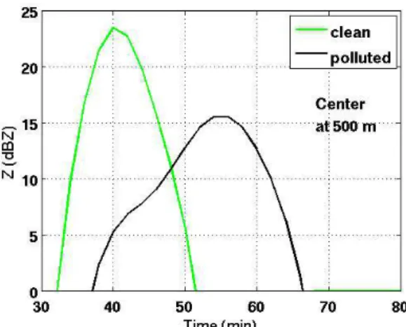
Fig. 11. The calculated radar reflectivity below cloud center at
500 m height for the clean cloud (green curve) and most polluted one (black curve).
Fig. 12. The mass mixing ratio below cloud center at 500 m height
for the clean cloud (green curve) and most polluted one (black curve).
a much smaller average size. Large drops do form in a pol-luted cloud (in much smaller number). These large drops, while falling, collect water mass very efficiently due to two reasons: (1) they have more water-mass to collect (the cal-culated integrals of the curves in Fig. 8 show a larger mass of the small mode in the polluted cloud case) (2) higher col-lection efficiency, due to larger variance in size between the large drops and the background smaller droplets. It results in larger and much fewer rain drops in the polluted cloud.
Below cloud base (Fig. 8b) at 52 min of simulation, only the large mode exists in the mass size distribution, for both clouds. The small-drop peak, which can be recognized above cloud base in the polluted cloud mass distribution (at 1200 m level, Fig. 8a), is reduced significantly below cloud base due to their evaporation. The distance of fall for complete evap-oration of drops smaller than 50 microns increases with the forth power of radius (Rogers and Yau., 1989), therefore the
Fig. 13. Accumulated rain (mm) as a function of the distance from
cloud center (100 m resolution) for cloud 1 (clean) – green columns, cloud 2 (800 cm−3) – red columns, cloud 3 (1600 cm−3) – black columns.
smallest drops are very susceptible to the subsaturated condi-tions below cloud base. The mass mixing ratios at these grid points are 0.7 g kg−1for the clean cloud and only 0.2 g kg−1
for the polluted one. The total number concentrations are 0.003 and 0.00009 cm−3, i.e., there is less mass mixing ratio,
and smaller drop concentrations, but because the reduction in drop concentration is much greater than the reduction in mass mixing ratio, the drops are larger in the polluted case.
The mean drop radius below cloud base has a significant impact on radar reflectivity calculations. Figure 11 presents the calculated radar reflectivity below the bases of clouds 1 and 3, 500 m above ground. It can be compared to the mass mixing ratio for this height, presented in Fig. 12 (the drop concentration at this height is larger below the clean cloud base at all times for which rain is falling). The two clouds present a different time evolution of radar reflectivity. This calculated parameter can be compared in the future to radar observations. By comparison to Fig. 12 it can be seen that there is a trend for the polluted cloud radar reflectivity val-ues towards higher valval-ues. The mass mixing ratio of the most polluted cloud becomes larger than the one of the clean cloud at 58 min but the calculated radar reflectivity becomes larger as early as 48 min into the simulation. The ratio between the maximum mass mixing ratio of the clean and most polluted cloud, is 3.9, and the ratio between the maximum radar re-flectivity values is only 1.5. These are because the sensitivity of the radar reflectivity to the presence of big drops (the radar reflectivity depends in the diameter to the 6th power). The larger drops of the most polluted cloud are shown in Fig. 10. So although the drop mass is significantly reduced by pollu-tion, the radar reflectivity difference is not as marked because of the presence of larger raindrops below cloud base in the polluted case.
The accumulated rain as a function of the distance from the center of the cloud (Fig. 13) demonstrates that, as expected,
O. Altaratz et al.: Aerosols’ influence on warm cumulus cloud 23 most of the rain accumulates below the central part of the
cloud for these no-shear axisymmetrical simulations. The differences between rain amounts collected on the ground in the clean and the polluted case become larger moving away from the center toward the peripheral regions below the clouds. In the middle of the cloud (grid point number 1) the ratio between the accumulated rain in the clean compared to the most polluted cloud is 2.7. At the margin (500 m from the center) this ratio is 21.9. Due to the entrainment and en-hanced evaporation at the margin of the polluted cloud, the rain accumulated on the ground below this region is much smaller than in the clean cloud.
4 Summary
The Tel Aviv University axisymmetrical cloud model was used to study the influence of aerosols on coastal convective clouds of moderate size.
The results show an enhanced evaporation process in the polluted clouds in comparison to the clean cloud; this is the case near cloud top and the lateral margins. At cloud top the evaporation process and the resultant downdrafts (mainly at the first stage of clouds’ lifetime) lead to a lower cloud top height in the polluted clouds in comparison to the clean cloud (Xue and Feingold, 2006). Most of the mass evaporated in the polluted cloud margins and top derives from the small drop mode due to their high surface area to volume ratio. The evaporation process at the lateral margins of the polluted clouds is of importance in determining the amount of cloud water in these regions and the amount of rain which falls from them. Due to these processes the width of the polluted clouds is smaller than for the clean clouds’ width during most of the simulation time (14–56 min). Only at the end of the dissipation stage (that happens earlier in the clean case) it reverses and the clean cloud becomes smaller in the mean horizontal width. The amount of rain from the polluted cloud is suppressed more near the cloud margins than under the cloud core (in a relative sense).
We have shown that unlike in the case of the small cloud droplets, the raindrops are larger in the polluted cloud. This is clearly the case below the cloud where only raindrops ex-ist. Inside the cloud, separation of the large-drop mode from the small one reveals that in the polluted cloud, the drops are larger due to a more efficient collision-coalescence process: fewer large drops collect more numerous, small drops, the latter resulting from an infusion of aerosol. It is expected that these large collector drops will exist in polluted clouds which produce rain. To verify that our results are not uniquely de-pendent on our initial conditions (temperature and humidity profiles and aerosol size distribution) we did several tests. 1) We changed the temperature and humidity profiles 2) re-moved the large aerosol mode (>4 µm). In all those test sim-ulations once the polluted cloud produced rain, the mean size of the polluted cloud rain drops was larger than the clean.
As expected, the polluted convective clouds precipitate less than clean clouds. Increasing the pollution concentra-tion, above the background level, from 0 to 1600 cm−3leads
to a decrease in the total rain volume on the ground by a factor of ∼3.5. Mean drop radius has a significant impact on radar reflectivity calculations. Comparison of the radar reflectivity to the mass mixing ratio shows there is a trend of the polluted-cloud radar reflectivity values towards higher values because of the sensitivity of the radar reflectivity to the presence of big drops.
Acknowledgements. O. Altaratz and I. Koren acknowledge the par-tial support of the ISF (grant 1355/06). A. Kostinski acknowledges support by the Weizmann Institute of Science, Israel and by the NSF grant ATM05-54670. Helpful discussions with D. Rosenfeld are acknowledged.
Edited by: G. McFiggans
References
Ackerman, A. S., Kirkpatrick, M. P., Stevens, D. E., and Toon, O. B.: The impact of humidity above stratiform clouds on indirect aerosol climate forcing, Nature, 432, 1014–1017, 2004. Albrecht, B. A.: Aerosols, cloud microphysics, and fractional
cloudiness, Science, 245, 1227–1230, 1989.
Coakley, J. A. and Walsh, C. D.: Limits to the aerosol indirect ra-diative effect derived from observations of ship tracks, J. Atmos. Sci., 59, 668–680, 2002.
Durkee, P. A., Noone, K. J., and Bluth, R. T.: The Monterey area ship track experiment, J. Atmos. Sci., 57, 2523–2541, 2000. Ferek, R. J., Hegg, D. A., Hobbs, P. V., Durkee, P., and Nielsen, K.:
Measurements of ship-induced tracks in clouds off the Washing-ton coast, J. Geophys. Res., 103, 23 199–23 206, 1998.
Ferek, R. J., Garrett, T., Hobbs, P. V, Strader, S., Johnson, D., Tay-lor, J. P., Nielsen, K., Ackerman, A. S., Kogan, Y., Liu, Q., Al-brecht, B., and Babb, D.: Drizzle suppression in ship tracks, J. Atmos. Sci., 57, 2707–2728, 2000.
Han, Q., Rossow, W. B., Zeng, J., and Welch, R.: Three different behaviors of liquid water path of water clouds in aerosol-cloud interactions, J. Atmos. Sci., 59, 726–735, 2002.
Jaenicke, R.: Aerosol physics and chemistry, Landolt-Brnstein Neue Serie 4b, 391–457, 1988.
Jiang, H., Xue, H., Teller, A., Feingold, G., and Levin, Z.: Aerosol effects on the lifetime of shallow cumulus, Geophys. Res. Lett., 33, L14806, doi:10.1029/2006GL026024, 2006.
Jiang, H. and Feingold, G.: The effect of aerosol on warm con-vective clouds: Aerosol-cloud-surface flux feedbacks in a new coupled large eddy model, J. Geophys. Res., 111, D01202, doi:10.1029/2005JD006138, 2006.
Khain, A., Rosenfeld, D., and Pokrovsky, A.: Aerosol impact on the dynamics and microphysics of deep convective clouds, Q. J. Roy. Meteor. Soc., 131, 2639–2663, 2005.
King, M. D., Radke, L. F., and Hobbs, P. V.: Optical properties of marine stratocumulus clouds modified by ships, J. Geophys. Res. Atmos., 98, 2729–2739, 1993.
Kogan, Y. L.: The simulation of a convective cloud in a 3-D model with explicit microphysics, Part I, Model description and sensi-tivity experiments, J. Atmos. Sci., 48, 1160–1189, 1991. Platnick, S., Durkee, P. A., Nielsen, K., Taylor, J. P., Tsay, S.-C.,
King, M. D., Ferek, R. J., Hobbs, P. V., and Rottman, J. W.: The role of background cloud microphysics in the radiative formation of ship tracks, J. Atmos. Sci., 57, 2607–2624, 2001.
Pruppacher, H. R. and Klett, J. D.: Microphsics of clouds, Reidel, 714 pp., 1978.
Ring, M. D., Radke, L. F., and Hobbs, P. V.: Optical properties of marine stratocumulus clouds modified by ships, J. Geophys. Res., 98, 2729–2739, 1993.
Radke, L. F., Coakley Jr., J. A., and Ring, M. D.: Direct and remote sensing observations of the effects of ships on clouds, Science, 246, 1146–1149, 1989.
Reisin, T., Levin, Z., and Tzivion, S.: Rain production in convective clouds as simulated in an axisymmetric model with detailed mi-crophysics, Part I, Description of the model, J. Atmos. Sci., 53, 497–519, 1996.
Rogers, R. R. and Yau, M. K.: A Short Course in Cloud Physics, 3rd ed., Pergamon, New York, 293 pp., 1989.
Teller, A. and Levin, Z.: The effects of aerosols on precipitation and dimensions of subtropical clouds, a sensitivity study using a numerical cloud model, Atmos. Chem. Phys., 6, 67–80, 2006, http://www.atmos-chem-phys.net/6/67/2006/.
Twomey, S.: Pollution and the planetary albedo, Atmos. Environ., 8, 1251–1256, 1974.
Twomey, S.: The influence of pollution on the shortwave albedo of clouds, J. Atmos. Sci., 34, 1149–1152, 1977.
Tzivion, S., Feingold, G., and Levin, Z.: An efficient numerical solution to the stochastic collection equation, J. Atmos. Sci., 44, 3139–3149, 1987.
Tzivion, S., Reisin, T., and Levin, Z.: Numerical Simulation of Hy-groscopic Seeding in a Convective Cloud, J. Appl. Meteorol., 33, 252–267, 1994.
Xue, H. and Feingold, G.: Large eddy simulations of tradewind cumuli, Investigation of aerosol indirect effects, J. Atmos. Sci., 63, 1605–1622, 2006.
Xue, H., Feingold, G., and Stevens, B.: Aerosol effects on clouds, precipitation, and the organization of shallow cumulus convec-tion, J. Atmos. Sci., in press, 2007.
Yin, Y., Levin, Z., Reisin, T. G., and Tzivion, S.: The effect of giant cloud condensation nuclei on the development of precipitation in convective clouds – A numerical study, Atmos. Res., 53, 91–116, 2000.
Yin, Y., Wurzler, S., Levin, Z., and Reisin, T. G.: Interactions of mineral dust particles and clouds, Effects on precipitation and cloud optical properties, J. Geophys. Res., 107(D23), 4724– 4738, 2002.
Zhao, M. and Austin, P. H.: Life cycle of numerically simulated shallow cumulus clouds, Part II, Mixing dynamics, J. Atmos. Sci., 62, 1291–1310, 2005.