HAL Id: insu-01298980
https://hal-insu.archives-ouvertes.fr/insu-01298980
Submitted on 19 Jul 2020
HAL is a multi-disciplinary open access
archive for the deposit and dissemination of
sci-entific research documents, whether they are
pub-lished or not. The documents may come from
teaching and research institutions in France or
abroad, or from public or private research centers.
L’archive ouverte pluridisciplinaire HAL, est
destinée au dépôt et à la diffusion de documents
scientifiques de niveau recherche, publiés ou non,
émanant des établissements d’enseignement et de
recherche français ou étrangers, des laboratoires
publics ou privés.
Three-dimensional full-kinetic simulation of the solar
wind interaction with a vertical dipolar lunar magnetic
anomaly
Jan Deca, Andrey Divin, Xu Wang, Bertrand Lembège, Stefano Markidis,
Mihály Horányi, Giovanni Lapenta
To cite this version:
Jan Deca, Andrey Divin, Xu Wang, Bertrand Lembège, Stefano Markidis, et al..
Three-dimensional full-kinetic simulation of the solar wind interaction with a vertical dipolar lunar magnetic
anomaly. Geophysical Research Letters, American Geophysical Union, 2016, 43 (9), pp.4136-4144.
�10.1002/2016GL068535�. �insu-01298980�
Three-dimensional full-kinetic simulation of the solar
wind interaction with a vertical dipolar
lunar magnetic anomaly
Jan Deca1,2,3, Andrey Divin4,5, Xu Wang1,2, Bertrand Lembège3, Stefano Markidis6, Mihály Horányi1,2, and Giovanni Lapenta7
1Laboratory for Atmospheric and Space Physics, University of Colorado Boulder, Boulder, Colorado, USA,2Institute for
Modeling Plasma, Atmospheres and Cosmic Dust, NASA/SSERVI, Boulder, Colorado, USA,3Laboratoire Atmosphères, Milieux, Observations Spatiales, Université de Versailles à Saint Quentin, Guyancourt, France,4Physics Department,
St. Petersburg State University, St. Petersburg, Russia,5Swedish Institute of Space Physics (IRF), Uppsala, Sweden, 6High Performance Computing and Visualization, KTH Royal Institute of Technology, Stockholm, Sweden,7Centre for
mathematical Plasma Astrophysics, Department of Mathematics, KU Leuven, Leuven, Belgium
Abstract
A detailed understanding of the solar wind interaction with lunar magnetic anomalies (LMAs) is essential to identify its implications for lunar exploration and to enhance our physical understanding of the particle dynamics in a magnetized plasma. We present the first three-dimensional full-kinetic electromagnetic simulation case study of the solar wind interaction with a vertical dipole, resembling a medium-size LMA. In contrast to a horizontal dipole, we show that a vertical dipole twists its field lines and cannot form a minimagnetosphere. Instead, it creates a ring-shaped weathering pattern and reflects up to 21% (four times more as compared to the horizontal case) of the incoming solar wind ions electrostatically through the normal electric field formed above the electron shielding region surrounding the cusp. This work delivers a vital piece to fully comprehend and interpret lunar observations, as we find the amount of reflected ions to be a tracer for the underlying field structure.1. Introduction
The Luna 2 mission discovered that the Moon, unlike the Earth, lacks a global magnetic field [Dolginov and
Pushkov, 1960]. Soon after the Apollo missions provided the first evidence of localized crustal magnetic fields.
These peculiar features are known as lunar magnetic anomalies (LMAs). LMAs are small with respect to the lunar radius (RL= 1738 km) and typical solar wind ion scales. Models based on low-altitude observations estimate LMA surface magnetic field strengths in between 0.1 and 1000nT [Mitchell et al., 2008; Richmond
and Hood, 2008; Tsunakawa et al., 2015]. Spacecraft and laboratory experiments have revealed a variety of
phenomena associated with these fields, including limb shocks, whistler and electrostatic solitary waves, reflected ions and energetic neutral atoms, the presence of electrostatic potentials above the magnetic struc-ture [Halekas et al., 2008; Hashimoto et al., 2010; Lue et al., 2011; Saito et al., 2012; Futaana et al., 2013; Wang
et al., 2012, 2013; Howes et al., 2015], and the formation of minimagnetospheres [Deca et al., 2014, 2015; Wieser et al., 2010; Vorburger et al., 2012; Bamford et al., 2012; Nishino et al., 2015].
Over the last decade, the evolution from magnetohydrodynamic [Harnett and Winglee, 2003; Shaikhislamov
et al., 2013, 2014; Xie et al., 2015] and hybrid [Kallio et al., 2012; Jarvinen et al., 2014; Fatemi et al., 2015] toward
full-kinetic simulations [Deca et al., 2014, 2015; Ashida et al., 2014] has made it abundantly clear that the solar wind-LMA interaction is highly nonadiabatic. The ability to investigate finite gyroradius effects and charge separation is therefore an absolute must to correctly describe the electron physics-dominated LMA environment.
Deca et al. [2014, 2015] studied the general mechanism and dynamics of the solar wind-LMA interaction
using a dipolar model with the dipole moment parallel to the lunar surface (hereafter the horizontal dipole model). They confirmed that LMAs may indeed be capable to locally shield the lunar surface under various upstream plasma conditions. They identified a population of backstreaming ions and the deflection of mag-netized electrons via the E × B drift motion. The synergy of both mechanisms results in the formation of a minimagnetosphere.
RESEARCH LETTER
10.1002/2016GL068535 Key Points:
• In contrast to a horizontal dipolar LMA, a vertical dipole cannot form a minimagnetosphere
• A ring-shaped weathering pattern is created and reflects up to 21% of the incoming solar wind ions
• The amount of reflected ions is a tracer for the underlying magnetic field structure
Correspondence to: J. Deca,
Citation:
Deca, J., A. Divin, X. Wang, B. Lembège, S. Markidis, M. Horányi, and G. Lapenta (2016), Three-dimensional full-kinetic simulation of the solar wind inter-action with a vertical dipolar lunar magnetic anomaly, Geophys. Res. Lett., 43, 4136–4144, doi:10.1002/2016GL068535.
Received 4 MAR 2016 Accepted 1 APR 2016
Accepted article online 5 APR 2016 Published online 12 MAY 2016
©2016. American Geophysical Union. All Rights Reserved.
Geophysical Research Letters
10.1002/2016GL068535
In this work we rotate the dipole axis by 90∘, having the dipole moment perpendicular to and directed toward the lunar surface, complementing the discussion to characterize the plasma interaction with a small-scale dipole model under partially magnetized plasma conditions in the interaction region. As most LMAs have irregular structures [Mitchell et al., 2008], a vertical dipole is the next vital piece needed to better understand the basic kinetic processes coupling LMAs with surface weathering and lunar swirls—high-albedo markings on the lunar surface. Eventually, the vertical and horizontal models will be combined for more realistic descrip-tions of LMAs. In particular, this analysis will help to evaluate the role of LMAs in the formation history of our Moon and crustal magnetic fields/space weathering on airless bodies in our solar system as it aids to correlate observed LMAs with lunar swirls [Hood and Williams, 1989; Blewett et al., 2011; Hemingway and Garrick-Bethell, 2012; Glotch et al., 2015].Understanding the kinetic physics around LMAs is not only critical to advance lunar science, also at Mars crustal magnetic fields are observed and believed to complicate the solar wind interaction with its atmo-sphere [Acuna et al., 1999]. In addition, artificial minimagnetoatmo-spheres might play an important role in future human space flight as well [Bamford et al., 2014].
2. Simulation Specifics
The implicit moment particle-in-cell code iPic3D [Markidis et al., 2010] has been developed for multiscale plasma simulations, with original studies focused on magnetic reconnection and recently optimized to study the interaction with bodies immersed in plasma. In this work two extra components are implemented on top of the standard code (The iPic3D code is publicly available on GitHub (https://github.com/CmPA/iPic3D).): (1) the ability to have an external field, B′, representing the anomaly, superimposed on the self-consistent
(internal) magnetic field B:
B′(r) = 𝜇0 4𝜋 (3(m⋅ (r − r 0))(r − r0) (r − r0)5 − m (r − r0)3 ) ,
with m the dipole moment (in Am2) and the source located at r
0and (2) electromagnetic open boundary
con-ditions accommodating a uniform drifting Maxwellian plasma through the computational domain with one of the boundaries acting as a perfect absorber representing the lunar surface (see Deca et al. [2015] for details). Currently, photoemission, secondary electron emission, and surface charging [Deca et al., 2013] are under active development for the electromagnetic version of the code. We argue that these physical mechanisms do not influence the main key points of this work.
Considering Cartesian coordinates, the YZ plane is chosen parallel to the lunar surface with the origin at the surface. The X axis is chosen perpendicular to the surface and antiparallel to the unperturbed solar wind flow. The following physical parameters are utilized, representing a situation close to quiet solar wind conditions: the plasma density is set nsw=3 cm−3, corresponding to an ion inertial length d
i∼130 km; the ion and electron temperatures are Tsw= Ti= Te=35 eV, and the solar wind velocity vsw= (−350, 0, 0) km s−1.
To simplify the magnetic structure of the interaction, we neglect any interplanetary magnetic field in this work. The dipole moment m = (Md, 0, 0), where Md=11.2 × 10¹²Am2, resembles the strongest component of the Reiner Gamma two-dipole model by Kurata et al. [2005], but in contrast, we place the dipole vector perpen-dicular to the lunar surface. The size of the simulation domain measures (Lx, Ly, Lz) = (0.625, 1.25, 1.25) di= (80, 160, 160) km. The absorbing surface is located at x = 0, and the dipole is placed at the center of the
YZ plane 13km below the outflow boundary. The grid size is Nx× Ny× Nz= 320 × 640 × 640 with 64 particles per cell per species initially. We use a reduced mass ratio of mi∕me=256, resulting in an electron skin depth
de= 0.0625 di= 32 Δx, with Δx = 254 m the grid spacing. The time step is chosen relative to the ion plasma frequency: Δt = 0.01875 𝜔−1
pi, with𝜔pi= 2.3 × 10³rad/s.
3. Analysis of the Electromagnetic Fields
When the solar wind plasma impinges on the LMA field, the vertical dipole model looses its “ideal” shape. In Figure 1 we show the resulting magnetic field configuration with respect to the initial setup after the simula-tion has reached steady state (after ∼10,000 time steps). Figure 1a shows the magnetic field strength at the surface including magnetic field lines generated in the vicinity of the origin ((x, y, z) = 0), whereas Figure 1b
Figure 1. Two-dimensional profiles of the magnetic and electric field configurations. Superimposed in black are
projected magnetic field lines. (a) Initial (left of the red marker) and final (right of the red marker) magnetic field magnitude in the YZ plane at the lunar surface. A blue arrow indicates the clockwise field line twist. (b) Initial (left of the red marker) and final, compressed configuration (right of the red marker) of the magnetic field magnitude in the XY plane through the dipole center. (c) The electric fieldxcomponent in the XY plane through the dipole center.
presents the configuration along the XY plane through the origin. Note that unlike for the horizontal dipole model, the configuration is cylindrically symmetric. From Figure 1 we find the vertical dipole both compressed (Figures 1b and 1c) and twisted in the clockwise direction looking down onto the surface (Figure 1a). The maximum magnetic field strength at the surface increases from 870 nT to 890 nT in the center of the cusp. The largest compression, however, is found 9 km away from the center where the field strength rises from roughly 470 to 520 nT at the surface. The field lines are being dragged (pushed down) onto the surface (Figure 1b). Concentrating on Figure 1a, we identify three distinct segments in the magnetic field lines projected onto the surface. Their structure is representative for the field in the entire simulation domain. Most central we observe a radially outward pointing segment where the dipole field dominates the electron dynamics (up to roughly 15 km from the center). Ions become magnetized only in the very center of the dipole cusp. The ion gyroradius reads ∼700 m at the surface in the cusp center. Between 15 and 50 km from the center the field lines are curved. In this region the electron population transitions from an unmagnetized (𝜌e∼10 km at 50 km) to a magnetized regime (𝜌e≲2 km below 15 km). Ions and electrons decouple, resulting in a net current density component, Jnet= Je+ Ji, pointing along the direction of flow toward the surface (Figure 2a). We call the lower boundary of this region the electropause (indicated with a red dash on the figure), the loca-tion where the electron kinetic (solar wind + thermal) pressure equals the magnetic pressure. Finally, the field lines originating from the dipole field connect to the boundaries of the simulation domain in the outermost segment. Note that in our simulation we have neglected the interplanetary magnetic field (IMF). The inclusion of various IMF magnitudes and orientations is under active investigation.
Figure 2c shows the generation of a circular current system in a clockwise direction when looking down on the surface. Both the ∇B and E × B drift steer the electron motion. Whereas the former dominates the interac-tion above x = 30 km, the latter drift mechanism is dominant within and directly above the electron shielding region (a region where mostly electrons are shielded away from the surface, leaving a positively charged area [Howes et al., 2015], see also the discussion of Figure 3 in the next paragraph) where a normal electric field exists (Figure 1c) due to charge separation. Above the electropause only a fraction of the electron population is magnetized, and hence, the circular (electron) current twists the magnetic field lines in a clockwise direction following the electron motion. Note that reversing the dipole moment would also reverse the twist direction. Figure 3 shows the density structure resulting from the vertical dipole configuration. Both the ion and electron charge density profiles (Figures 3b and 3c) and prevail a higher density bulge (up to 3.5 times the free-stream solar wind density) near the origin as they are funneled (and possibly reflected) within the magnetic cusp. Observe as well the population of particles pushed sideways (away from the cusp center) along the com-pressed magnetic field. This is most pronounced in the electron charge density profile (Figure 3b) as electrons are magnetized in this area of the simulation domain and a large fraction cannot reach the surface [Howes et al., 2015]. Adding up the ion and electron charge density at the surface results in the profile shown in Figure 3a.
Geophysical Research Letters
10.1002/2016GL068535
Figure 2. Two-dimensional profiles of the net current density components (Je+ Ji) in the XY plane. (a) x, (b) y, and (c) z components. Superimposed in black are projected magnetic field lines. The height of the electropause above the lunar surface at the dipole center is indicated with a red dash.
Around the central bulge, dominated by the electron population (for most of the electrons the mirror point finds itself below the surface), we observe a positively charged ring formed because up to 70% of the lighter plasma species is prevented from reaching the surface as they travel along the magnetic field into the cusp. The associated electric field in the XY plane is displayed in Figure 1c. Most ions travel almost undisturbed to the surface in this region [Howes et al., 2015], resulting in a ring visible in the density structure up to 5 km above the surface under the adopted plasma conditions. We anticipate that reducing the solar wind pressure will increase the height of the electron shielding region.
Figure 3. Two-dimensional profiles of the net charge density (𝜌net=𝜌e+𝜌i) in the YZ plane at the (a) lunar surface and
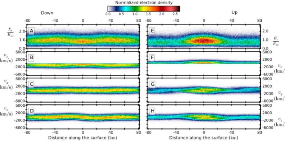
Figure 4. (a–d) Electron and (e–h) ion distribution functions along the profile parallel to the solar wind flow and
through the center of the dipole. Figures 4a and 4e show the total energy distribution normalized to the solar wind energy. Figures 4b–4d and 4f–4h hold the velocity distributions along the three Cartesian axes of the simulation domain normalized to the solar wind density.
4. Analysis of the Energy and Velocity Distribution Functions
In this section we concentrate on the ion and electron energy/velocity distributions along the direction of flow and across the simulation domain parallel to the surface. Figure 4, showing the distributions along the line (Y =0, Z=0), is constructed by grouping all particles per species within a 6 × 6 cell (1.524 × 1.524 km) domain into 50 uniform energy/velocity bins according to their position along the axis. The axis itself is divided into 200 position bins. Figures 5 and 6 are constructed analogously, but this time dividing along the Y axis at
x = 25 km, parallel to the surface.
4.1. Along the Direction of Flow
Figure 4 depicts the line parallel to the dipole axis and through the dipole center hence perpendicular to the lunar surface. Down to 25 km above the lunar surface the energy and velocity profiles are largely undisturbed. Moving closer to the surface, the electron total energy profile shows a steady 50% increase toward the surface starting from 15 km altitude. In this region the electron perpendicular velocity distribution widens (Figures 4c and 4d) as the electron gyroorbit tightens with increasing magnetic field strength toward the surface. Below 10 km the electron population is accelerated into the cusp (Figure 4b) by the charge-separation normal electric field (Figure 1c). Note that the broad near-surface distribution in vyand vzis the typical signature of magnetic mirroring (but cut short by the absorbing surface).
Figure 5. Electron distribution functions along the profile parallel to the surface and along the Y axis atx = 25km above the surface, split up into the (a–d) downstreaming and (e–h) upstreaming populations. Figures 5a and 5e show the total energy distribution normalized to the solar wind energy. Figures 5b–5d and 5f–5h hold the velocity distributions along the three Cartesian axes of the simulation domain normalized to the solar wind density.
Geophysical Research Letters
10.1002/2016GL068535
Figure 6. Ion distribution functions along the profile parallel to the surface and along the Y axis atx = 25km above the surface, split up into the (a–d) downstreaming and (e–h) upstreaming populations. Figures 6a and 6e show the total energy distribution normalized to the solar wind energy. Figures 6b–6d and 6f–6h hold the velocity distributions along the three Cartesian axes of the simulation domain normalized to the solar wind density.
In contrast to the energy profile for the electron population, the ion energy distribution (Figure 4e) super-imposes two distinct components consistent with an almost undisturbed clean Maxwellian plasma, i.e., the flowing solar wind plasma perpendicular to the lunar surface and a beam of electrostatically reflected ions. Evaluating the vxdistribution (Figure 4f ) we find a significant reflected component all the way up to the inflow boundary of the simulation domain, accounting for 21% of the ion population, i.e., 21% of the incoming ions are reflected when looking directly above the cusp region (integrating over a cylinder with diameter 1.524 km and height 254 m). Note, this does not implicate that ions are retroreflected, we merely capture the distribu-tion passing our line of sight as ions are electrostatically reflected by the normal electric field (Figure 1c). The very clear cutoff in the reflected velocity component, not exceeding the chosen upstream solar wind speed, can easily be identified and is in qualitative agreement with observations [Lue et al., 2014; Saito et al., 2012;
Fatemi et al., 2014]. We find, hence, that both a horizontal and vertical dipole are capable of reflecting a
sig-nificant fraction of the ion population. In our setup the vertical dipole is about a factor 4 more efficient under the chosen plasma conditions as compared to the horizontal dipole model [Deca et al., 2014, 2015]. This fact can be attributed to the different electric field structures of both setups. Whereas the horizontal model scat-ters the reflected ions mostly under a shallow angle with respect to the surface, the semitoroidal structure of the vertical case focuses the reflected ions more upward [Deca et al., 2016].
Finally, due to the absence of a significantly strong normal electric field directly above the cusp, similar to the charge separation field generated when a minimagnetosphere forms around a horizontal dipole [see Deca
et al., 2015, Figure 5], the ion population is not significantly slowed down before reaching the surface through
the dipole cusp. A vertical dipole configuration, i.e., a dipole moment perpendicular to the lunar surface, therefore, does not form a minimagnetosphere in the traditional sense [Lin et al., 1998] (a density cavity within a higher density halo shielding the lunar surface from the impinging solar wind plasma). Most ions and electrons will be absorbed at the lunar surface before being reflected/deflected away from the surface within the cusp region. The electron shielding region surrounding the cusp, however, forms a ring where both plasma species are to some degree prevented from reaching the lunar surface. In the best shielded region 71% of the electron population is shielded away versus 28% of ions. Note, the electron shielding efficiency is much lower as compared to a horizontal configuration where almost the entire electron population cannot reach the surface within the density halo [Deca et al., 2014, 2015]. The ion shielding efficiency, on the other hand, is similar as the normal electric field above the electron shielding region reaches a comparable magnitude,
Ex,max∼150mV
m [Figure 1c versus Figure 5 in Deca et al. [2015].
4.2. Parallel to the Surface
To characterize the behavior of the ion and electron populations at various radial distances from the dipole center, we generate a similar series of 1-D profiles as in Figure 4, but parallel to the surface. This time, however, we split the distributions in their downstreaming and upstreaming components, taking the sign of
the lunar surface hence above the positively charged density ring and the complex ion reflection region (Figures 5 and 6).
Figures 5a–5d show the energy and velocity distribution functions of the downstreaming electrons and indi-cate little deflection from the initial drifting Maxwellian distribution released into the simulation domain along the entire width of the box. The small rotational component inevitably invoked by the magnetized electrons interacting with the vertical dipole structure is most clearly seen in the vzdistribution (the wobble at ±20 km). In the upstreaming component (Figures 5e–5h), on the other hand, the bulge in the central cusp region is readily observed and consists partially of reflected electrons spiraling (Figures 5g and 5h) upward out of the cusp on top of the initial distribution. The reflected population cannot be identified as a separate compo-nent in Figures 4a–4d, because the thermal spread of the electron distribution is larger than the magnitude of the upstreaming component. It is therefore quickly reintegrated into the bulk distribution. With exception of the central bulge, the upstreaming electrons are 25% less energetic as compared to their downstreaming counterparts.
As the ion population is nonmagnetized at 25 km above the lunar surface, the downstreaming popula-tion keeps its perfect drifting Maxwellian shape (Figures 6a–6d). The upstreaming/reflected populapopula-tion (Figure 6e–6h), on the other hand, shows that the lion’s share of the ions is reflected close to the center axis of the vertical dipole with energies on the lower side of the energy distribution as compared to the initialized downstreaming population. Similar to the electrons, also the reflected ion population shows a spiraling tendency upward as they are reflected by the electrostatic electric field (Figure 1c). Close to the surface and the cusp all particles are briefly “magnetized” to some degree. Traveling away from the surface, their trajec-tories straighten out again as the magnetic field magnitude drops, leaving the ion with a significant velocity component oblique to the solar wind direction. The E × B drift motion is greatest in this region and most likely the main responsible for the spiraling tendency of the reflected ions. A detailed study of the electron and ion reflection processes around dipolar LMAs is under active investigation.
5. Concluding Remarks
In this work we have discussed the solar wind interaction with a vertical dipole resembling a medium-size vertical LMA using a three-dimensional full-kinetic electromagnetic particle-in-cell approach. For simplicity the case study was performed without IMF. We find that the magnetic field is compressed by the solar wind pressure and twisted in a clockwise direction as the ion and electron populations decouple above the lunar surface. In contrast to a horizontal dipole, the vertical magnetic field structure does not form a minimagne-tosphere. We find that roughly 21% of the impinging ion plasma is reflected, close to a factor 4 more than the typical numbers obtained for a horizontal dipole [Deca et al., 2014, 2015]. Both numbers are within the ranges observed by the most recent lunar missions and can possibly be used as tracers to reveal the underly-ing magnetic structure [e.g., Halekas et al., 2013; Lue et al., 2014; Vorburger et al., 2015, and references therein]. In addition, they indicate the ranges to expect for more general simulation setups and parameter studies. Of course, not a single observed LMA can be characterized as a single dipole. Nevertheless, understand-ing the details of the idealized scenarios first is a must to built more comprehensive models in the future. Investigating the structural outcome and particle dynamics of the latter might shed new, clarifying light on the suggested correlations between LMAs and lunar swirls, high-albedo markings, and space weathering, in general. In particular, studying the weathering patterns predicted by simulations with a realistic magnetic field model will help evaluate the importance of the solar wind standoff mechanisms.
References
Acuna, M. H., et al. (1999), Global distribution of crustal magnetization discovered by the Mars Global Surveyor MAG/ER Experiment, Science, 284, 790–793, doi:10.1126/science.284.5415.790.
Ashida, Y., H. Usui, I. Shinohara, M. Nakamura, I. Funaki, Y. Miyake, and H. Yamakawa (2014), Full kinetic simulations of plasma flow interactions with meso- and microscale magnetic dipoles, Phys. Plasmas, 21(12), 122903, doi:10.1063/1.4904303.
Bamford, R. A., B. Kellett, W. J. Bradford, C. Norberg, A. Thornton, K. J. Gibson, I. A. Crawford, L. Silva, L. Gargaté, and R. Bingham (2012), Minimagnetospheres above the lunar surface and the formation of lunar swirls, Phys. Rev. Lett., 109(8), 81101, doi:10.1103/PhysRevLett.109.081101.
Bamford, R. A., et al. (2014), An exploration of the effectiveness of artificial mini-magnetospheres as a potential solar storm shelter for long term human space missions, Acta Astronaut., 105(2), 385–394, doi:10.1016/j.actaastro.2014.10.012.
Blewett, D. T., E. I. Coman, B. R. Hawke, J. J. Gillis-Davis, M. E. Purucker, and C. G. Hughes (2011), Lunar swirls: Examining crustal magnetic anomalies and space weathering trends, J. Geophys. Res., 116, E02002, doi:10.1029/2010JE003656.
Acknowledgments
This work was supported in part by NASA’s Solar System Exploration Research Virtual Institute (SSERVI): Institute for Modeling Plasmas, Atmosphere, and Cosmic Dust (IMPACT). Resources supporting this work were provided by the NASA High-End Computing (HEC) Program through the NASA Advanced Supercomputing (NAS) Division at Ames Research Center. This work also utilized the Janus supercomputer, which is supported by the National Science Foundation (award CNS-0821794) and the University of Colorado Boulder. The Janus supercomputer is a joint effort of the University of Colorado Boulder, the University of Colorado Denver, and the National Center for Atmospheric Research. This research has received funding from the European Commission’s FP7 Program under the grant agreement EHEROES (project 284461, www.eheroes.eu). Test simulations were conducted on the computational resources provided by the PRACE Tier-0 project 2013091928 (SuperMUC supercomputer). Part of this work was inspired by discussions within International Team 336: “Plasma Surface Interactions with Airless Bodies in Space and the Laboratory” at the International Space Science Institute, Bern, Switzerland. Access to the raw data may be provided upon motivated request to J.D.
Geophysical Research Letters
10.1002/2016GL068535
Deca, J., G. Lapenta, R. Marchand, and S. Markidis (2013), Spacecraft charging analysis with the implicit particle-in-cell code iPic3D, Phys. Plasmas, 20(10), 102902, doi:10.1063/1.4826951.
Deca, J., A. Divin, G. Lapenta, B. Lembège, S. Markidis, and M. Horányi (2014), Electromagnetic particle-in-cell simulations of the solar wind interaction with lunar magnetic anomalies, Phys. Rev. Lett., 112(15), 151102, doi:10.1103/PhysRevLett.112.151102.
Deca, J., A. Divin, B. Lembège, M. Horányi, S. Markidis, and G. Lapenta (2015), General mechanism and dynamics of the solar wind interac-tion with lunar magnetic anomalies from 3-D pic simulainterac-tions, J. Geophys. Res. Space Physics, 120, 6443–6463, doi:10.1002/2015JA021070. Deca, J., A. Divin, X. Wang, B. Lembège, S. Markidis, G. Lapenta, and M. Horányi (2016), Solar wind interaction with lunar magnetic
anomalies: Vertical vs. horizontal dipole, in Lunar and Planetary Science Conference, Lunar and Planetary Science Conference, vol. 47, p. 1065, LPI Contribution No. 1903, Woodlands, Tex.
Dolginov, S. S., and N. V. Pushkov (1960), Magnetic field of the outer corpuscular region, in Proceedings from the 6th International Cosmic Ray Conference, vol. 3, edited by S.I. Syrovatsky, p. 30, Moscow, Russia.
Fatemi, S., M. Holmström, Y. Futaana, C. Lue, M. R. Collier, S. Barabash, and G. Stenberg (2014), Effects of protons reflected by lunar crustal magnetic fields on the global lunar plasma environment, J. Geophys. Res. Space Physics, 119, 6095–6105, doi:10.1002/2014JA019900. Fatemi, S., C. Lue, M. Holmström, A. R. Poppe, M. Wieser, S. Barabash, and G. T. Delory (2015), Solar wind plasma interaction with
Gerasimovich lunar magnetic anomaly, J. Geophys. Res. Space Physics, 120, 4719–4735, doi:10.1002/2015JA021027.
Futaana, Y., S. Barabash, M. Wieser, C. Lue, P. Wurz, A. Vorburger, A. Bhardwaj, and K. Asamura (2013), Remote energetic neutral atom imaging of electric potential over a lunar magnetic anomaly, Geophys. Res. Lett., 40, 262–266, doi:10.1002/grl.50135.
Glotch, T. D., J. L. Bandfield, P. G. Lucey, P. O. Hayne, B. T. Greenhagen, J. A. Arnold, R. R. Ghent, and D. A. Paige (2015), Formation of lunar swirls by magnetic field standoff of the solar wind, Nat. Commun., 6, 6189, doi:10.1038/ncomms7189.
Halekas, J. S., G. T. Delory, D. A. Brain, R. P. Lin, and D. L. Mitchell (2008), Density cavity observed over a strong lunar crustal magnetic anomaly in the solar wind: A mini-magnetosphere?, Planet. Space Sci., 56, 941–946, doi:10.1016/j.pss.2008.01.008.
Halekas, J. S., A. R. Poppe, J. P. McFadden, and K.-H. Glassmeier (2013), The effects of reflected protons on the plasma environment of the moon for parallel interplanetary magnetic fields, Geophys. Res. Lett., 40, 4544–4548, doi:10.1002/grl.50892.
Harnett, E. M., and R. M. Winglee (2003), 2.5-D fluid simulations of the solar wind interacting with multiple dipoles on the surface of the Moon, J. Geophys. Res., 108, 1088, doi:10.1029/2002JA009617.
Hashimoto, K., et al. (2010), Electrostatic solitary waves associated with magnetic anomalies and wake boundary of the Moon observed by KAGUYA, Geophys. Res. Lett., 37, L19204, doi:10.1029/2010GL044529.
Hemingway, D., and I. Garrick-Bethell (2012), Magnetic field direction and lunar swirl morphology: Insights from Airy and Reiner Gamma, J. Geophys. Res., 117, E10012, doi:10.1029/2012JE004165.
Hood, L. L., and C. R. Williams (1989), The lunar swirls—Distribution and possible origins, in Lunar and Planetary Science Conference Proceedings, vol. 19, edited by G. Ryder and V. L. Sharpton, pp. 99–113, Cambridge Univ. Press, Houston, Tex.
Howes, C. T., X. Wang, J. Deca, and M. Horányi (2015), Laboratory investigation of lunar surface electric potentials in magnetic anomaly regions, Geophys. Res. Lett., 42, 4280–4287, doi:10.1002/2015GL063943.
Jarvinen, R., M. Alho, E. Kallio, P. Wurz, S. Barabash, and Y. Futaana (2014), On vertical electric fields at lunar magnetic anomalies, Geophys. Res. Lett., 41, 2243–2249, doi:10.1002/2014GL059788.
Kallio, E., et al. (2012), Kinetic simulations of finite gyroradius effects in the lunar plasma environment on global, meso, and microscales, Planet. Space Sci., 74, 146–155, doi:10.1016/j.pss.2012.09.012.
Kurata, M., H. Tsunakawa, Y. Saito, H. Shibuya, M. Matsushima, and H. Shimizu (2005), Mini-magnetosphere over the Reiner Gamma magnetic anomaly region on the Moon, Geophys. Res. Lett., 32, L24205, doi:10.1029/2005GL024097.
Lin, R. P., D. L. Mitchell, D. W. Curtis, K. A. Anderson, C. W. Carlson, J. McFadden, M. H. Acuna, L. L. Hood, and A. Binder (1998), Lunar surface magnetic fields and their interaction with the solar wind: Results from lunar prospector, Science, 281, 1480, doi:10.1126/science.281.5382.1480.
Lue, C., Y. Futaana, S. Barabash, M. Wieser, M. Holmström, A. Bhardwaj, M. B. Dhanya, and P. Wurz (2011), Strong influence of lunar crustal fields on the solar wind flow, Geophys. Res. Lett., 38, L03202, doi:10.1029/2010GL046215.
Lue, C., Y. Futaana, S. Barabash, M. Wieser, A. Bhardwaj, and P. Wurz (2014), Chandrayaan-1 observations of backscattered solar wind protons from the lunar regolith: Dependence on the solar wind speed, J. Geophys. Res. Planets, 119, 968–975, doi:10.1002/2013JE004582. Markidis, S., G. Lapenta, and Rizwan-uddin (2010), Multi-scale simulations of plasma with iPIC3D, Math. Comput. Simul., 80(7), 1509–1519,
doi:10.1016/j.matcom.2009.08.038.
Mitchell, D. L., J. S. Halekas, R. P. Lin, S. Frey, L. L. Hood, M. H. Acuña, and A. Binder (2008), Global mapping of lunar crustal magnetic fields by Lunar Prospector, Icarus, 194, 401–409, doi:10.1016/j.icarus.2007.10.027.
Nishino, M. N., Y. Saito, H. Tsunakawa, F. Takahashi, M. Fujimoto, Y. Harada, S. Yokota, M. Matsushima, H. Shibuya, and H. Shimizu (2015), Electrons on closed field lines of lunar crustal fields in the solar wind wake, Icarus, 250, 238–248, doi:10.1016/j.icarus.2014.12.007. Richmond, N. C., and L. L. Hood (2008), A preliminary global map of the vector lunar crustal magnetic field based on Lunar Prospector
magnetometer data, J. Geophys. Res., 113, E02010, doi:10.1029/2007JE002933.
Saito, Y., M. N. Nishino, M. Fujimoto, T. Yamamoto, S. Yokota, H. Tsunakawa, H. Shibuya, M. Matsushima, H. Shimizu, and F. Takahashi (2012), Simultaneous observation of the electron acceleration and ion deceleration over lunar magnetic anomalies, Earth Planets Space, 64, 83–92, doi:10.5047/eps.2011.07.011.
Shaikhislamov, I. F., V. M. Antonov, Y. P. Zakharov, E. L. Boyarintsev, A. V. Melekhov, V. G. Posukh, and A. G. Ponomarenko (2013), Mini-magnetosphere: Laboratory experiment, physical model and Hall MHD simulation, Adv. Space Res., 52, 422–436, doi:10.1016/j.asr.2013.03.034.
Shaikhislamov, I. F., Y. P. Zakharov, V. G. Posukh, A. V. Melekhov, V. M. Antonov, E. L. Boyarintsev, and A. G. Ponomarenko (2014), Experimental study of a mini-magnetosphere, Plasma Phys. Controlled Fusion, 56(2), 25004, doi:10.1088/0741-3335/56/2/025004.
Tsunakawa, H., F. Takahashi, H. Shimizu, H. Shibuya, and M. Matsushima (2015), Surface vector mapping of magnetic anomalies over the Moon using Kaguya and Lunar Prospector observations, J. Geophys. Res. Planets, 120, 1160–1185, doi:10.1002/2014JE004785. Vorburger, A., P. Wurz, S. Barabash, M. Wieser, Y. Futaana, M. Holmström, A. Bhardwaj, and K. Asamura (2012), Energetic neutral atom
observations of magnetic anomalies on the lunar surface, J. Geophys. Res., 117, A07208, doi:10.1029/2012JA017553.
Vorburger, A., P. Wurz, S. Barabash, M. Wieser, Y. Futaana, A. Bhardwaj, and K. Asamura (2015), Imaging the South Pole-Aitken basin in backscattered neutral hydrogen atoms, Planet. Space Sci., 115, 57–63, doi:10.1016/j.pss.2015.02.007.
Wang, X., M. Horányi, and S. Robertson (2012), Characteristics of a plasma sheath in a magnetic dipole field: Implications to the solar wind interaction with the lunar magnetic anomalies, J. Geophys. Res., 117, A06226, doi:10.1029/2012JA017635.
Wang, X., C. T. Howes, M. Horányi, and S. Robertson (2013), Electric potentials in magnetic dipole fields normal and oblique to a surface in plasma: Understanding the solar wind interaction with lunar magnetic anomalies, Geophys. Res. Lett., 40, 1686–1690, doi:10.1002/grl.50367.
Wieser, M., S. Barabash, Y. Futaana, M. Holmström, A. Bhardwaj, R. Sridharan, M. B. Dhanya, A. Schaufelberger, P. Wurz, and K. Asamura (2010), First observation of a mini-magnetosphere above a lunar magnetic anomaly using energetic neutral atoms, Geophys. Res. Lett., 37, L05103, doi:10.1029/2009GL041721.
Xie, L., L. Li, Y. Zhang, Y. Feng, X. Wang, A. Zhang, and L. Kong (2015), Three-dimensional hall mhd simulation of lunar minimagnetosphere: General characteristics and comparison with chang’E-2 observations, J. Geophys. Res. Space Physics, 120, 6559–6568,