Comparing a ballistic trajectory to terrain using digital elevation data

(1)

Comparing a Ballistic Trajectory to Terrain using Digital Elevation Data by

Jeremy R. Henry

Submitted to the Department of Electrical Engineering and Computer Science in Partial Fulfillment of the Requirements for the Degrees of

Bachelor of Science in Electrical Engineering and Computer Science and

Master of Science in Electrical Engineering and Computer Science

at the

Massachusetts Institute of Technology February 1995

The author hereby grants to MIT permission to reproduce and to distribute publicly paper and electronic copies of this thesis

document in whole or in part.

Signature of Author _

Certified by , -

-Accepted by

Prof. Tomaozano-Pbrez

Massachusetts Institute of, Tehnology Thpsi SIAdvisor 1

rgenthaler

Massach s Institute of Technology Chairman,\Committee on Graduate Students

Eng.

MASSACHUSETTS INSTITUTE ...I. • - , rl '•V

(2)

(3)

CONTENTS LIST OF TABLES 5 LIST OF FIGURES 7 ACKNOWLEDGMENT 9 ABSTRACT 11 1. INTRODUCTION 13 2. TECHNICAL BACKGROUND 14 2.1. Previous Research 14 2.2. Coordinate Systems 14 2.3. DTED 22 2.4. Ballistic Trajectories 25

2.5. Computational Environment Constraints 28

3. BASIC SYSTEM DESCRIPTION 29

3.1. System Inputs 30

3.2. System Components 31

3.3. System Output 37

3.4. System Analysis and Evaluation 38

4. TRUTH MODEL COMPARISON SYSTEM 52

4.1. Basic Description 52

4.2. Truth Model System Components 53

4.3. Analysis of Truth Model 60

5. POINT TO POINT COMPARISON SYSTEM 71

5.2. Point to Point System Components 71

5.3. Analysis of Point to Point System 72

6. CRANE COMPARISON SYSTEM 77

6.2. Crane System Components 78

6.3. Analysis of Crane System 80

7. OCTREE COMPARISON SYSTEM 88

7.2. Octree System Components 89

7.3. Analysis of Octree System 92

8. DISCUSSION AND CONCLUSIONS 99

8.1. System Comparison 99

8.2. Conclusions 105

8.3. Additional Discussion 105

(4)

(5)

LIST OF TABLES

Table 1. Post Spacing of DTED by Latitudinal Zone ... 23

Table 2. DTED Memory Requirements per Block Size ... ... 36

Table 3. General description of test cases ... 43

Table 4. Curve-fitting polynomials to the altitude component of trajectories... 64

Table 5. Curve-fitting polynomials to the crossrange component of trajectories ... 66

Table 6. Truth Model Accuracy Results for Test Case #1 ... 67

Table 7. Truth Model Accuracy Results for Test Case #2 ... .... 67

Table 8. Truth Model Accuracy Results for Test Case #3 ... .... 67

Table 14. Truth Model Efficiency Results ... ... ... 70

Table 15. Accuracy Results of Point To Point System for Test Case #1 ... 73

Table 23. Point To Point System Efficiency Results ... 76

Table 24. Maximum Error per Test Case due to Linear Interpolation ... 81

Table 25. Accuracy Results of Crane System for Test Case #1 ... 84

Table 33. Crane System Efficiency Results... 87

Table 34. Accuracy Results of Octree System for Test Case #1 ... 93

(6)

Table 42. Octree System Efficiency Results... 97

Table 43. Test Results on Octree Construction... 98

Table 44. Timing Results of Comparison Systems ... 00

Table 45. Accuracy Results of Comparison Systems ... 101

(7)

LIST OF FIGURES

Figure 1. Earth Centered Coordinate System ... ... ... 15

Figure 2. Geodetic Latitude ... ... 16

Figure 3. Geodetic Longitude ... ... 17

Figure 4. Organization of Basic Comparison System... ... 29

Figure 5. Swatch encompassing all possible ballistic trajectories ... . 32

Figure 6. Block selection based on a swatch ... ... ... 33

Figure 7. Intersection Points... ... 38

Figure 8. Subsystems which contribute to time usage. ... .... .. 40

Figure 9. F ractal P lot... 54

Figure 10. DTED map with square marked for fractal interpolation ... 55

Figure 11. Location of sample points in relation to the reference location ... 56

Figure 12. Recursive midpoint interpolation using four neighbors ... 58

Figure 13. Fractal Interpolation of Rough Terrain ... ... 61

Figure 14. Fractal Interpolation of Medium Terrain ... ... 61

Figure 15. Fractal Interpolation of Smooth Terrain ... 61

Figure 16. Surfaces produced with various fractal parameters... ... . 62

Figure 17. Altitude comparison of actual trajectory to interpolated trajectory ... 63

Figure 18. Crossrange comparison of actual trajectory to interpolated trajectory ... 65

Figure 19. Example Comparison Points in Crane Comparison System ... 77

Figure 20. Division of volume into octants... 88

Figure 21. Octree data structure ... ... 89

Figure 22. Graphic Representation of Timing Results...100

Figure 23. Graphic Representation of Maximum Horizontal Error...102

(8)

(9)

ACKNOWLEDGMENT

The author wishes to thank Professor Tomas Lozano-PBrez of the Massachusetts Institute of Technology and Mr. Dan Hogan for advising this project.

For technical guidance the author wishes to thank Mr. Bennie Burnsed, Mrs. Anne Helgerman, Mr. Matthew Crane, Mr. Peter Samsel, Mr. Eric Helgerman, Mr. Wayne Marzotto, and Mr. Cotton Seed.

For their assistance and resources the author wishes to thank Mr. Jason Henry, Miss Rima AiYun Woo, and Mr. Jin S. Choi.

For their love and support the author wishes to thank Mrs. Lulu S. Henry, Mr. and Mrs. John W. Henry, and Miss Jody Henry.

(10)

(11)

Comparing a Ballistic Trajectory to Terrain using Digital Elevation Data by

Jeremy R. Henry

Submitted to the Department of Electrical Engineering and Computer Science in Feb. 1995 in partial fulfillment of the Requirements for the Degrees of Bachelor or Science in Electrical Engineering and Computer Science and

Master of Science in Electrical Engineering and Computer Science

ABSTRACT

A system is needed which will compare a terrestrial launch ballistic trajectory to a digital map of the underlying terrain in order to determine the points at which the trajectory intersects the terrain. Three candidate comparison algorithms are presented. First, a brute-force algorithm which compares the elevation of the trajectory at one meter intervals to an interpolated terrain elevation. Second, an

algorithm which only checks the trajectory elevation at points at which it passes between two existing terrain elevation sample points. Third, an algorithm which divides the problem space using an octree data structure. The trajectory is checked

against every data structure volume through which it passes.

It is desired to determine which of the candidate algorithms displays the optimal performance using criteria such as computation time, memory usage, and accuracy. In order to determine the optimal approach, each of the candidate algorithms is implemented as a computer program. The implementations are then analyzed and compared using a series of test cases. The results of the comparison are described. The optimal system is shown to be an approach using an octree data structure. This system displays satisfactory space and time efficiency while achieving above-average accuracy. The approach employs a divide and conquer strategy, and concentrates its resources on checking the most interesting portions of the trajectory.

(12)

(13)

1. INTRODUCTION

A system is needed which is able to compare predicted ballistic trajectories to the earth's surface in order to determine if and where the trajectory intersects the terrain. The ballistic trajectories are simple terrestrial launch parabolic paths which are represented as a series of points in space. Previous methods of checking trajectory involved painstaking and often inaccurate manual examination of available contour maps. With the introduction and widespread availability of digital terrain elevation databases, it becomes possible to automate the process, increasing both accuracy and efficiency. However, several different approaches to performing the actual comparison are possible, and little is known of their relative efficiency or accuracy. Efficiency, measured in terms of time and memory consumed by the comparison algorithm, can only be considered in the context of a specific type of processing environment. For the purpose of this project, a single sequential processor with a limited amount of random access memory is used.

The accuracy of a comparison algorithm is much more difficult to analyze then the efficiency. One obvious method of testing accuracy is to perform field tests and observations. However this method is outside the scope of this project. Furthermore, this method is made infeasible by the desire to determine not only where a trajectory path enters the terrain, but also the point at which it exits the terrain obstruction after passing through it. So instead of field testing, an artificial terrain is constructed based on the data in the existing terrain elevation database. This high resolution, artificially created terrain is then used along with an exacting, brute-force algorithm to determine the exact location of terrain intersections down to the necessary level of accuracy. The intersection locations resulting from this approach are then used as the baseline against which the accuracy of all other comparison methods are evaluated.

In an attempt to find a best possible comparison method, three possible algorithms were identified, each of which has the capability to perform the desired comparison. In selecting the candidates, it was desired to exercise a variety of possible techniques. The description of an approach was not limited to the comparison itself, but also included any processing which may be performed on the trajectory or the terrain elevation data. Divide-and-conquer as opposed to brute-force iterative methods were also explored.

The overall goal of this project was then to implement the candidate comparison systems on a representative computer architecture, and then to analyze and compare the performance of the different approaches over a series of test cases. The objective being to find the model which offers the best performance in terms of processing time, memory usage, and accuracy.

(14)

2. TECHNICAL BACKGROUND

2.1. Previous Research

Numerous articles have been published on the use of digital terrain elevation data for a wide variety of applications. These include watershed determination [LEE92],

planetary surface rendering (for satellite testing) [YOKOY89], perspective terrain rendering [BARBE91] [MILLE86], and others. However, it appears as though very little if any research has been done on the use of digital terrain data to determine intersection points between the terrain and arbitrary paths defined in space, whether these paths describe the flight of meteors, re-entrant satellites, ground-launched ballistic projectiles, low-flying aircraft, etc. This may be due to the relatively scarce availability of digital terrain elevation databases. The database used in this project, DTED, is a product of the United States Department of Defense, and as yet has only a limited distribution.

It may also be observed that very little research has been done on applications which use elevation data quantitatively rather than qualitatively. This is most likely due to the lack of accuracy inherent in most available digital elevation databases. The DTED product used for this project also has serious accuracy limitations. These limitations were summarily ignored in order to minimize the scope of the project and still obtain meaningful results.

2.2. Coordinate Systems

This project is concerned primarily with the determination of terrestrial locations and elevations. There are numerous coordinate systems with which terrestrial locations can be described, and this project employs three of them; Earth-Centered Cartesian Coordinate System, WGS 84 Geodetic Coordinate System, and a local Trajectory Coordinate System. Many of the terms used in the description of coordinate systems are used in different contexts by different authors. In order to insure clarity, the three coordinate systems listed above as well as conversions among the three are described in detail in this section.

2.2.1. Earth-Centered Cartesian Coordinate System

The Earth-Centered Cartesian Coordinate System is the most basic of the coordinate systems used to describe terrestrial locations. Locations are defined using three coordinates. These coordinates represent distances along the three axes of a regular three-dimensional Cartesian coordinate system. The axes are labeled as U-V-W and distances along them are measured in meters.

The origin of the system is at the center of the reference ellipsoid, where the reference ellipsoid is the geometric object approximating the earth. The center of this reference ellipsoid is very nearly equal to the gravitational center of the earth. The 'U' axis lies where the plane of the Greenwich meridian (zero degrees longitude)

intersects the equatorial plane (zero degrees latitude). The 'W' axis lies along the earth's axis of rotation in the direction of the north pole. The 'V' axis lies so that the axes U-V-W form a right-handed coordinate system.

(15)

Equator

Pole

I 11111i IVI0 l luJI ll

Figure 1. Earth Centered Coordinate System 2.2.2. WGS 84 Geodetic Coordinate System

This is a terrestrial coordinate system based on the WGS 84 ellipsoid. As mentioned before, the reference ellipsoid is a geometric object approximating the earth. The WGS 84 ellipsoid is a specific example of a reference ellipsoid. The WGS 84 Geodetic Coordinate System locates points on or near the surface of the ellipsoid using three coordinates. These coordinates are referred to as latitude (represented as

4),

longitude (represented as X), and elevation (represented as h).

The WGS 84 ellipsoid is an ellipsoid of revolution with specific values defined for its semi-major and semi-minor axes. For many applications, a perfect sphere is sufficient as a model of the earth. However, for applications which require greater accuracy, the ellipsoid of revolution is commonly used. The ellipsoid of revolution is the geometric volume obtained by rotating an ellipse around one of its axes (in this case, its minor axis).

The ellipsoid is used for geodesy because it more closely approximates the actual shape of the earth. The earth is not perfectly spherical in shape. It is elliptical, widest at the equator and flattened on the poles due to the apparent centrifugal acceleration caused by the earth's rotation. The ellipsoid of revolution represents the shape which the earth's oceans would conform to if they were free to adjust to the effects of gravity and the earth's rotation, ignoring the tidal effects of the sun and moon and any localized gravitational anomalies in the earth itself.

Because the ellipsoid of revolution can be derived entirely from a single ellipse, the ellipsoid can be completely defined using the same two parameters used to describe the ellipse. There are several choices as to which two parameters to use to describe the ellipsoid. For simplicity, this project will generally use the lengths of the semi-major and semi-minor axes.

(16)

semi-major axis: semi-minor axis:

a = 6,378,137.000 meters b = 6,356,752.314 meters

Using these two parameters, several other parameters can be determined which will be useful in different cases. These include:

flattening: f = a- b = 1 /298.257223563

a

semi-major eccentricity squared: semi-minor eccentricity squared:

a

2 _- _b2

ea 2 2 2 ea 2f - f2

b - b 12 - ea 2 _{(1 - f)2}

The WGS 84 Geodetic Coordinate System locates points on this ellipsoid using three coordinates: latitude, longitude, and elevation.

The geodetic latitude is the angle which the normal to the reference ellipsoid at the specified point makes with the plane of the equator. Latitudes are defined between -90 and +90 degrees with the positive latitude lying north of the equator.

Normal to Ellipsoid ;tion

Figure 2. Geodetic Latitude

The geodetic longitude is the angle formed by the projection of the radius vector of the specific point onto the equatorial plane and the vector from the polar axis to the

reference (Greenwich) meridian. Longitudes are defined between -180 and +180 degrees with the positive longitudes lying east of the reference meridian.

Elliosc

South Pole

(17)

Ellipsoid

Vector in Question Reference Meridian

Figure 3. Geodetic Longitude

The geodetic elevation is the height of the specified point above or below the surface of the ellipsoid (mean sea level). This height is measured along a line which is normal to the surface of the ellipsoid at the point in question. Note also that the line normal to the surface of the ellipsoid represents the direction of the combined accelerations due to gravity and the earth's rotation. Thus the definition of height in this manner agrees with our general concept of "up" and "down".

2.2.3. Trajectory Coordinate System

The Trajectory Coordinate System is a three dimensional Cartesian coordinate system. Locations in this coordinate system are specified by three coordinates; Downrange, Vertical, and Crossrange. The Trajectory Coordinate System is oriented such that the plane described by the downrange and crossrange axes is tangent to the reference ellipsoid at the location of the trajectory launch. Thus the origin of the Trajectory Coordinate System is at the longitude and latitude of the launch point with an elevation of h = 0. The downrange axis is oriented in the direction of the terminating point of the trajectory.

Consider an arbitrary trajectory. The Downrange axis lies in a plane which is tangent to the reference ellipsoid at the location of the launch. It is oriented in the direction of the terminating point of the trajectory. The Vertical axis is normal to the ellipsoid at the location of the launch. Its direction is away from the center of the ellipsoid, or "up". The Crossrange axis is oriented so that the Downrange-Vertical-Crossrange axes form a right-handed coordinate system. If the launch point of the trajectory has an elevation of h which is not equal to zero (or sea level), then the trajectory, instead of initiating from (downrange = 0, vertical = 0, crossrange = 0), would instead initiate from the point (downrange = 0, vertical = h, crossrange = 0).

(18)

To fully specify a location in the Trajectory Coordinate System requires more than simply the Downrange, Crossrange, and Vertical coordinates. It is also necessary to specify the location and orientation of the Trajectory Coordinate System itself. The location is specified by the coordinate of the origin of the Trajectory Coordinate System in either Earth-Centered Cartesian Coordinates or in WGS 84 Geodetic Coordinates. The orientation is specified by the azimuth of the Downrange axis in radians. The "azimuth" is the angle which the Downrange axis projected onto the reference ellipsoid forms with a line on the reference ellipsoid which originates from the origin of the Trajectory Coordinate System and passes through the north pole. Any angle measured in this way is referred to as an "azimuth".

This Trajectory Coordinate System earns its name from the fact that this is the coordinate system in which the trajectory points are originally determined by the ballistic model.

2.2.4. Conversions Between Coordinate Systems

It is often necessary to convert the representation of a point from one coordinate system to another. These conversions are described in detail below. Unless otherwise stated, these conversions are derived independently or taken from the following sources [MILD] [VANIC86].

2.2.4.1. Converting Earth-Centered Cartesian to WGS 84 Geodetic

A location is specified in the Earth-Centered Cartesian Coordinate system by the coordinates (U, V, W). It is desired to convert this representation to the (4, X, h) or (latitude, longitude, elevation) coordinates of the WGS 84 Geodetic Coordinate System.

Calculation of the longitude is fairly straight-forward.

=2 -atan

_U+P

V

Note however that the equation breaks down (a divide by zero is attempted) when U+P = 0. This case corresponds to a point which lies on the international date line (1800 E longitude). In this case the negative U value is exactly offset by the positive P value. So when U+P = 0 then X = ir (1800 E longitude).

The computation of the geodetic latitude requires an iterative solution. The following solution comes from Rapp [RAPP84]. Rapp goes on to state that for terrestrial applications the solution converges to 0.1 millimeter of accuracy after only one iteration. As all of the applications of this procedure are terrestrial, one iteration of this algorithm is presented as a closed-form solution.

a-W

PO

_{=atan( b-P} W + eb2 b - sin3

PO

tan 0o = p a e 2 2 . o P-a ea acos 0 1 =atan ((1- f ) tan ) SW +eb2 -b- sin3

_P

1 = a tan -a- cos3

(19)

Where : a = semi-major axis of WGS 84 ellipsoid b = semi-minor axis of WGS 84 ellipsoid

P = VU2 + V2 _{= distance from the polar axis}

ea2 = semi-major eccentricity of the WGS 84 ellipsoid

eb2 _{= semi-minor}_{eccentricity of the WGS 84 ellipsoid}

f = flattening of the WGS 84 ellipsoid

Note that the equation for Do breaks down (a divide by zero is attempted) when P = 0. As P is the distance from the polar axis, this case corresponds to a point which lies on the north or south pole. So if W > 0 then = n i2 (900 N latitude). If W < 0 then

I

=

-n/2 (900 S latitude).

The calculation of h follows from the calculation of latitude.

a N=

l- ea2 . Sin2)

h= P-N

Cos

Where : a = semi-major axis of WGS 84 ellipsoid P = VU2 + V2 = distance from the polar axis

ea2 ₌_semi-major_{eccentricity of the WGS 84 ellipsoid}

Note that the equation for h breaks down when 0 = n or -7c. This corresponds to the points on the north or south poles. Thus in polar regions, the following equation is preferred:

h= -N+ea2.N

sin 0

2.2.4.2. Converting Earth-Centered Cartesian to Trajectory

A location is specified in the Earth-Centered Cartesian Coordinate system by the coordinates (U, V, W). It is desired to convert this representation to the (dr, v, cr) (or (downrange, vertical, crossrange)) coordinates of the Trajectory Coordinate System. This conversion requires that the orientation and location of the Trajectory Coordinate System be specified. This is accomplished by the location of the trajectory system origin given in geodetic coordinates (4o, Xo, ho), and the azimuth of the downrange axis given in radians (ODR).

Step 1. Subtract the U, V, W offsets to the location of the trajectory system origin from the (U, V, W) coordinate of the location to obtain the (AU, AV, AW) values from the origin of the Trajectory Coordinate System to the location.

a

N=

1 - ea2 - _sin2₍

0)

SAU 'U ((N+ ho)-cos(dO) cos(X₀)

AV = V (N+ ho).cos(4Oo). sin(X0 )

(20)

Step 2. Rotate by ko about the W axis to align the U axis to point toward the polar axis.

M

m -cos(X 0) -sin(X 0) 0')( AU)

n -sin(x,) cos( ₀,) 0 AV

AW 0 0 1 AW

In this step, the m axis is parallel to the U-V plane and points directly towards the polar axis. The n axis also parallel to the U-V plane and is perpendicular to the m axis such that the m-AW-n axes form a right-handed coordinate system.

Step 3. Align the m-n plane with the N-E plane by rotating about the n axis by 0o.

'

N)I

sin(O4)

0 cos(°

0 )

m

V=

-cos(O

0

)

0 sin(O

0

)

n

SE0 1 0 )AW)

Step 4. Rotate the North-Vertical-East coordinate system to coincide with the downrange-vertical-crossrange coordinate system by rotating about the Vertical axis by ODR.

r

dr')

cos(ODR) sin(oDR)

vI=

0

1

0 I

V

cr,) -sin(ODR) o CoS(ODR)

),

E)

Result. The matrices from steps 2-4 can be combined into the following matrix (note that the components of the matrix are given in a shortened representation to aid presentation).

dr

-cos

ksin

o

_-cos

o

_{- sinX}

-

_{sin -sinX sin}

O

_cos

8 +

_cos

_Xsin

_cos

4 _s

_cos

_'(

_AU"

v = cos c - os sink -cos 4 sin

j

AV

cr) cos k . sin o. sin6 -sink .cos6 sink -sin .sin6 +cos .- cos6 - cos 4 . sinO) AW)

2.2.4.3. Converting WGS 84 Geodetic to Earth-Centered Cartesian

A location is specified in the WGS 84 Geodetic Coordinate System by the coordinates

(4,

X, h) or (latitude, longitude, elevation). It is desired to convert this representation to the (U, V, W) of the Earth-Centered Cartesian Coordinate System.

a N= 1- ea2 si2() U= (N+ h) cos(o) cos(6) V=(N+ h). cos(4) ) sin(6) W =(N- (1 - e2) + h) .sin(4)

(21)

2.2.4.4. Converting WGS 84 Geodetic to Trajectory

A location is specified in the WGS 84 Geodetic Coordinate System by the coordinates

(0, X, h) (or (latitude, longitude, elevation)). It is desired to convert this representation to the (dr, v, cr) (or (downrange, vertical, crossrange)) coordinates of the Trajectory Coordinate System. This conversion requires that the orientation and location of the Trajectory Coordinate System be specified. This is accomplished by the location of the trajectory system origin given in geodetic coordinates (Oo, X0, ho), and the azimuth of the downrange axis given in radians (tDR).

This conversion is not performed directly. Instead, the Earth-Centered Cartesian Coordinate System as an intermediary. First convert from the WGS 84 Geodetic Coordinate System to the Earth-Centered Cartesian Coordinate System as described in Section 2.2.4.3. Then convert the resulting (U, V, W) coordinates to the Trajectory Coordinate System using the conversion described in Section 2.2.4.2.

2.2.4.5. Converting Trajectory to Earth-Centered Cartesian

A location is specified in the Trajectory Coordinate by the coordinates (dr, v, cr) (or (downrange, vertical, crossrange)). It is desired to convert this representation to the (U, V, W) coordinates of the Earth-Centered Cartesian Coordinate System. The conversion from the Trajectory Coordinate System also requires that the orientation and location of the Trajectory Coordinate System be specified. This is accomplished by the location of the trajectory system origin given in geodetic coordinates (0o, ko, ho), and the azimuth of the downrange axis given in radians (ODR).

Step 1. Convert the point to a North-Vertical-East coordinate system by rotating about the Vertical axis by 8DR.

V 0 1 0 v

EJ sin(ODR) 0 Cos(ODR) cr

I

Step 2. Align the dr-cr plane with the U-V plane by rotating about the E axis by Oo.

' m ( 'sin(o 0 ) -cos(0o) 0) WN'

n

0

0 1 V

AW) Lcos(0o) sin(o) 0 E

In this step, the m axis is parallel to the U-V plane and points directly towards the polar axis. The n axis also parallel to the U-V plane and is perpendicular to the m axis.

Step 3. Rotate by

[

X, about the W axis to align the m axis with U.

AU-

(-cos(X

0

)

-sin(x

0

)

0)

(

m

AV = -sin( 0o) cos(ko) 0 n

AW 0 0 1,1 tAW)

Result. The matrices from steps 1-3 can be combined into the following matrix (note that the components of the matrix are given in a shortened representation to aid presentation).

(22)

SAU

(-cos-

sinO-cosO- sink sinO cosk-coso cos ksino-sinO-sinX cosO6

(dr

AV = - sink sin .cos +cosX.sin0 sink cos sink. sin • sin +cos kcos6

1

AW cos -cos 0 sin 0 -cos -sin 0, cr)

Step 4. Add the U, V, W offsets to the location of the trajectory system origin to obtain the (U, V, W) coordinates.

a N=

SU'

(

AU

**(N+ho).-cos(*,) cos(X)'**

V =

AV

+ (N+

h

₀

)cos(

₀

)

-sin(X

₀

)

W AW (N.(1-ea2)+ ho)sin(go)

2.2.4.6. Converting Trajectory to WGS 84 Geodetic

A location is specified in the Trajectory Coordinate by the coordinates (dr, v, cr) (or (downrange, vertical, crossrange)). It is desired to convert this representation to the

(4,

X, h) or (latitude, longitude, elevation) coordinates of the WGS 84 Geodetic Coordinate System. The conversion from the Trajectory Coordinate System also requires that the orientation and location of the Trajectory Coordinate System be specified. This is accomplished by the location of the trajectory system origin given in geodetic coordinates (04, X0, ho), and the azimuth of the downrange axis given in

radians (ODR).

There is no way to perform this conversion directly. Instead, it is necessary to use the Earth-Centered Cartesian Coordinate System as an intermediary. First convert from the Trajectory Coordinate System to the Earth-Centered Cartesian Coordinate System as described in Section 2.2.4.5. Then convert the resulting (U, V, W) coordinates to the WGS 84 Geodetic Coordinate System using the conversion described in Section 2.2.4.1.

2.3. Digital Terrain Elevation Data

The digital elevation data which will be used in this project is the Department of Defense standard product, the Digital Terrain Elevation Data (DTED). This data is produced by the Defense Mapping Agency in accordance with Military Specification MIL-D-89001 [MIL89]. The format of DTED is described in detail in the military specification for DTED, but an overview of that format will be presented here.

2.3.1. DTED Organization

DTED is a raster format product in which the elevation of the earth's surface is sampled at discrete points called "posts". At each post, a measurement is taken between the elevation of the terrain and the elevation of the WGS 84 spheroid. This measurement is essentially the height above (or below) sea level of the terrain. These post elevations are then grouped into blocks called "cells". A cell contains a two-dimensional array of post elevations which covers an area one degree of latitude by one degree of longitude. Each cell is labeled by the WGS 84 geodetic coordinate of its south-west corners. The cells are always referenced to integral degree values of latitude and longitude.

(23)

The posts are located in a regular grid pattern of rows and columns where rows correspond to lines of latitude and columns correspond to lines of longitude. The rows and columns fall along integral seconds of latitude or longitude. As stated previously, the southwest corner of each cell lies at an integral degree value of latitude and longitude. Therefore the west-most column and the south-most row or DTED posts also falls at an integral degree value of latitude or longitude. The remaining rows and columns of the cell are evenly spaced at an integral number of seconds apart. For example, the rows may be every three seconds of latitude apart and the columns every six seconds of longitude apart.

2.3.2. DTED Variation

Because of the irregular spacing of the lines of latitude and the convergence at the poles of the lines of longitude, the posts are not spaced regularly on the surface of the earth. The variation between lines of latitude is not severe, and therefore DTED ignores this variation. To account for the longitudinal variation, which becomes quite severe as we move from the equator towards the poles, DTED divides both the northern and southern hemispheres into 5 latitudinal zones. The longitudinal post spacing is different in each of the 5 zones. This helps to alleviate the greater part of the variation, but minor variation in longitudinal post spacing still occurs within each zone. These zones are described in Table 1.

DTED Level 1 DTED Level 2

Zone Latitude Longitude Latitude Longitude

Latitude Spacing Spacing Spacing Spacing

800_{N to 90}0_N _{3 sec. of lat. 18 sec. of long.} _{1 sec. of lat.} _{6 sec. of long.}

750N to 80oN 3 sec. of lat. 12 sec. of long. 1 sec. of lat. 4 sec. of long.

70°N to 750N 3 sec. of lat. 9 sec. of long. 1 sec. of lat. 3 sec. of long.

500_{N to 70oN} _{3 sec. of lat.} _{6 sec. of long.} _{1 sec. of}_lat. _{2 sec. of long.}

00 to 50ON 3 sec. of lat. 3 sec. of long. 1 sec. of lat. 1 sec. of long.

500S to 0" 3 sec. of lat. 3 sec. of long. 1 sec. of lat. 1 sec. of long.

700S to 50°S 3 sec. of lat. 6 sec. of long. 1 sec. of lat. 2 sec. of long. 750S to 700S 3 sec. of lat. 9 sec. of long. 1 sec. of lat. 3 sec. of long.

800S to 750_S _{3 sec. of lat. 12 sec. of long.} _{1 sec. of lat.} _{4 sec. of long.}

900S to 800S 3 sec. of lat. 18 sec. of long. 1 sec. of lat. 6 sec. of long. Table 1. Post Spacing of DTED by Latitudinal Zone

Note that DTED is defined between 900S and 90ON latitude. In practice, this project will only deal with latitudes between 800_{S and 84}0_{N latitude. Although it will not be} discussed further here, these boundaries are due to the limitations of the Universal Transverse Mercator (UTM) system which is only defined between 800_{S and 84}0_N latitude.

(24)

2.3.3. DTED Accuracy

The DTED is not 100% accurate. As stated above, the DTED is organized into blocks called "cells". Each of these cells measures 1 degree longitude by 1 degree latitude. The accuracy of the DTED is specified separately for each cell. The accuracy specifications consist of four values. These are: absolute horizontal accuracy, absolute vertical accuracy, point to point horizontal accuracy, point to point vertical

accuracy.

Absolute accuracy specifications measure the accuracy of the DTED with respect to the true earth terrain elevation. An absolute vertical accuracy value of x meters indicates that the post described in the DTED is within x meters of the altitude of the actual terrain with 90% probability. Likewise an absolute horizontal accuracy value of

x meters indicates that a piece of terrain of the given elevation exists within x meters

of the indicated location with 90% probability.

Relative accuracy specifications measure the accuracy of any single DTED measurement with respect to surrounding DTED measurements. A relative vertical accuracy value of y meters indicates that if the DTED specifies that adjacent posts A and B are z meters apart vertically, then the actual points on the earth which correspond to points A and B are actually (z-y) to (z+y) meters apart with 90% probability.

The accuracy of the DTED affects the accuracy of the comparison system. However, for the purposes of this project, these accuracy values will be ignored. Since it is impossible, barring actual field observation, to determine the nature or biases of the DTED inaccuracies, it will be assumed that the DTED values are correct as listed in the database.

2.3.4. DTED Versions

There are two versions of DTED. These are DTED Level 1 and DTED Level 2. The formats of these two versions are very similar. Their only difference is in the density of the data which they contain. DTED Level 1 is less dense than DTED Level 2. Level 1 is based on a latitude post spacing of 3 arcseconds and longitude post spacing of 3, 6, 9, 12, and 18 arcseconds (the variation occurs across the five latitudinal zones). Level 2 is based on latitude post spacing of 1 arcsecond and longitude post spacing of 1, 2, 3, 4, and 6 arcseconds (again the variation occurs across the five latitudinal zones).

A system which uses DTED must be able to handle both versions of DTED. Furthermore, cells of the two different versions may be interleaved.

Currently, DTED Level 2 has not reached the stage of widespread production and distribution. For this reason, DTED Level 2 will not be available for use on this project. Although it may be possible to simulate DTED Level 2 by appropriate interpolation DTED Level 1 data, it is unknown how closely the result would resemble actual Level 2 data. Therefore, no DTED Level 2, either real or simulated, will be

used on this project. However, all algorithms and implementations must still be able to handle interleaved sections of DTED Level 1 and Level 2.

(25)

2.4. Ballistic Trajectories

The ballistic trajectories which are to be compared to the DTED represent the path which a spin-stabilized ballistic projectile traces in space as it leaves the ground, arches up to apogee, and then falls again to the earth. In a vacuum this path would be a perfect parabola. However, the introduction of atmosphere and meteorological effects causes the path to diverge from this ideal. There are several algorithms and models which may be used to determine the path of a spin-stabilized projectile in an atmosphere. The model which is used on this project as well as the factors which affect it are described below.

2.4.1. Ballistic Model

The trajectories to be checked will be generated by a ballistic trajectory model described by Mastrey in her 1989 paper "Generation and Evaluation of a Ballistic Algorithm Development Model" [MASTR89]. Mastery's work is based on the trajectory model algorithm described in "A Modified Point Mass Trajectory Model for Rocket-Assisted Artillery" [BRL79]. This ballistic trajectory model is well documented and several implementations of the model have already been produced. Therefore the implementation of the model will not be addressed. However, the model is very general in that it allows many parameters to affect the flight of the projectile. Addressing all possible variations in ballistic trajectories is beyond the scope of this project, and so several of the available parameters to the ballistic model will be ignored or left constant. Each of the factors which affect the trajectory and the manner in which it will be handled in this project is addressed individually below: 2.4.1.1. Projectile

The general ballistic model can simulate an unlimited number of different types of spin-stabilized projectiles. All that is required for the model to handle an arbitrary projectile is a collection of physical and ballistic characteristics of that projectile. This information includes such Information as weight, drag, center-of-gravity, etc.

For this project, a single projectile type will be used. This projectile is the most basic type of projectile in that it is non-assisted, non-base-bleed, and single-staged.

The term "assisted" refers to rocket-assisted projectiles. These projectiles burn a self-contained propellant after initial launch in order to gain or maintain velocity during flight. The projectile which will be used in this project is non-assisted which means that its only source of motive power is from the initial launch. After the launch, the projectile is free-flying.

The term "base-bleed" refers to a class of projectiles which bleed a gas from their base during some stage of their flight in order to decrease drag. The projectile which will be used in this project is non-base-bleed which means that during the entire flight of the projectile, it will be affected by drag.

The term "single-stage" refers to a class of projectiles which act and are acted upon homogeneously throughout all portions of the flight. Other projectiles may change the composition of the projectile in mid-flight, thus altering the ballistic and physical characteristics of the projectile.

2.4.1.2. Meteorological Conditions

The general ballistic model allows the air temperature, air density, wind direction, and wind speed to be defined for 26 different layers of the atmosphere.

(26)

For this project, a single set of meteorological conditions will be used. This single set is referred to as the standard MET which has wind velocities of zero at every atmospheric layer.

2.4.1.3. Earth Model

The earth model parameter of the ballistic model determines whether the apparent Coriolis force acting on the projectile in flight will be taken into account. The Coriolis force has only a minor effect on the flight of the projectile, especially on shorter trajectories, and therefore the ballistic model is able to ignore the effect, if so

indicated, in order to speed up processing.

For this project the apparent Coriolis force will be taken into account by the ballistic model. Because the Coriolis force is dependent on the direction of travel of the projectile, as well as the latitude of the launch location, this means that trajectories which are similar in launcher elevation or launch velocity are none-the-less not interchangeable. It is therefore not feasible to calculate and store all possible trajectories before-hand.

2.4.1.4. Launch Conditions

As the projectile is non-assisted and there are no winds in the meteorological data, the launch supplies the only motive force to the projectile, and thus the launch conditions completely determine the trajectory which the projectile will follow. The launch conditions consist of the following factors: geodetic latitude of the launch location, height of launch above sea level, azimuth of launch, launcher elevation, and launch velocity.

The geodetic latitude of the launch location is necessary in computing the apparent Coriolis force acting on the projectile.

The height of the launch above sea level is used to determine the distance from the projectile to the center of gravity of the earth. This distance is needed to determine the magnitude of the earth's gravity acting on the projectile.

The azimuth of launch is necessary in that it allows the model to calculate the apparent Coriolis force acting on the projectile. The Coriolis force is a function of

(among other things) the direction of travel of the projectile in relation to the earth. The launch elevation of the launch is measured in radians above (or below) the

horizontal. The horizontal is defined to be a plane which is tangent to the earth's spheroid at the location of launch. For the purposes of this project, only launch elevations between -3 and 85 degrees from the horizontal will be considered.

The launch velocity is a single value which indicates the velocity of the projectile in three dimensional space in the direction of travel in meters per second. For the purposes of this project, only launch velocities between 100 and 1500 meters per second will be considered.

(27)

2.4.2. Trajectory Representation

The ballistic model produces a set of location coordinates which represent discrete points in the path of the trajectory. An average trajectory contains from 100 to 200 of these points. Extremely short distance trajectories may contain less than 100 points, while longer trajectories, or trajectories which terminate a substantial distance below the height of origin, may contain more than 200 points. The location coordinates are originally calculated in the Trajectory Coordinate System but they are made available in the form of WGS 84 Geodetic Coordinates as well.

The trajectory points are not uniformly spaced in either the downrange direction or in any other dimension. The distance between points is actually a function of the current acceleration of the projectile which is continuously varying over the course of the trajectory.

While it can be assumed that the projectile will pass through each of the location coordinates during its flight, the location of the projectile at any points between two adjacent trajectory points is undefined. However, given that there are no winds in the meteorological dataset and that the Coriolis force has a very minute affect on the path of the projectile, the only major forces acting on the projectile while in flight are gravity and the viscosity of the atmosphere. This makes it possible to predict that the projectile follows a roughly parabolic curve in the space between known points.

2.4.3. Trajectory Characteristics

The model which will be used is deterministic. That is, there are no random variables used in the computation of the trajectory, and therefore the results obtained from the ballistic model are reproducible. Thus it is possible to determine characteristics of trajectories and count on these characteristics holding true for future trajectories as well.

All trajectories calculated using the ballistic model have the same general shape. The trajectory curves downward according to gravity and to the right owing to the spin stabilization of the projectile and the fact that the projectile tips, or pitches over towards the earth as it flies (i.e., upon launch the nose of the projectile is pointing up while upon landing the nose of the projectile is pointing down).

As stated previously, the trajectory points are originally calculated in the Trajectory Coordinate System. One useful aspect of this representation is that the trajectory may be considered to be a function of the downrange dimension. That is, for each downrange value from zero (the launch point) to the impact point (the trajectory exists only between these bounds), there is a unique projectile location in both the crossrange and altitude dimensions.

Another useful aspect of the trajectory coordinate system representation is that the trajectory path may be decomposed into two separate functions; altitude as a function of downrange, and crossrange as a function of downrange. These functions are independent of one another and thus may be addressed separately. Both of these functions tend to resemble parabolic curves.

(28)

2.5. Computational Environment Constraints

This project will address the difficulties encountered when the trajectory / terrain comparison is performed in a real-time embedded system. The comparison system will therefore be subjected to a set of timing and memory constraints which may be typical of an embedded processing environment.

The implementation model against which the algorithms described in this project are analyzed consists of a single sequential processor with a limited amount of random access memory. The memory available to this processor is divided into three parts: code memory, data memory, and stack memory. The code memory is limited to 1 megabyte. However, all of the models described in this paper fall well under this limitation. The data memory consists of heap memory which is used to store static data structures as well as data which is too large to be stored on the stack, such as the DTED. The amount of data memory used by each comparison system will be monitored during test case runs. The stack memory is limited to 1 megabyte. The amount of stack memory used by the comparison systems will not be closely monitored like the data memory usage. Instead, the memory initially allocated for stack usage will be limited to 1 megabyte, and the run-time system will indicate if this maximum is exceeded. However, it is projected that 1 megabyte of stack space is quite sufficient for the needs of the comparison systems described in this paper. The time to perform the trajectory / terrain comparison is not limited in any way, but the time taken required by a comparison system to perform the actual comparison will factor into its evaluation.

The accuracy with which the trajectory / terrain comparison is performed is required to be accurate to within 100 meters in the horizontal direction in order to be considered "correct". The computational environment affects accuracy by dictating the data types which are available. The data types available on the model processor consist of a 2 byte signed integer, a 4 byte signed long integer, and an 8 byte floating point type

(29)

3. BASIC SYSTEM DESCRIPTION

The primary objective of this project is to analyze and evaluate three different comparison systems in order to determine which system performs the trajectory /

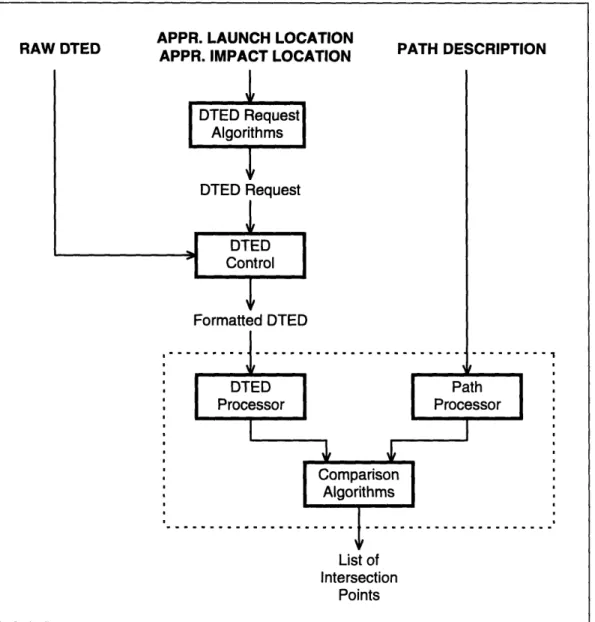
terrain comparison in the least amount of time while still observing memory and accuracy requirements. Each of the comparison systems has access to the same input data and is required to produce the same type of output data. In composition, each system has roughly the same organization and structure. This organization is graphically represented in Figure 4.

APPR. LAUNCH LOCATION

APPR. IMPACT LOCATION PATH DESCRIPTION

List of Intersection

Points

Figure 4. Organization of Basic Comparison System

This diagram shows the inputs to a comparison system, the five blocks of processing which must be performed, and the eventual output of the system. Each of these components is described below.

29

(30)

3.1. System Inputs

As indicated in Figure 4, the basic comparison system has three inputs. These are: raw DTED, the approximate launch and impact locations, and a description of the trajectory path. Each of these inputs is described individually below.

3.1.1. Raw DTED

The raw DTED is one of the basic inputs to a comparison system. It consists of the DTED data files which reside on the original DTED CDs. The format of these data files corresponds to the description found in the military specification on DTED [MIL89]. This format has been discussed previously.

A single DTED data file in its original format contains far more data that could ever be needed to perform a single trajectory comparison. Therefore, certain portions of DTED are selected for use by the comparison system and only these sections are stored and used by the comparison system.

3.1.2. Approximate Launch and Impact Locations

The approximate launch and impact locations are two of the basic inputs to a comparison system. Each approximate location is a geodetic coordinate (without an elevation component) which indicates the actual location of the launch or impact point to within 1 kilometer. In order to put a reasonable limit on the size of the problem space, the distance between the approximate launch and impact points is limited to 50 kilometers.

The approximate launch and impact locations are needed to determine what portions of DTED will be loaded from the raw DTED files into main memory. These values are only approximations of the actual launch and impact points because problem is defined such that the actual locations are not known until after the DTED has been loaded into main memory. This is too late for the actual values to be used in determining the necessary portions of DTED to actually load into main memory.

3.1.3. Path Description

The description of the trajectory path is one of the basic inputs to a comparison system. A path description consists of a set of between 2 and 500 projectile locations. Each location is represented in both the Trajectory Coordinate System as well as the WGS 84 Geodetic Coordinate System. Each location value specifies the position of the projectile at some point of the trajectory.

As has been stated previously, the path which the projectile follows between the points given in the path description is unknown, and can only be approximated.

Due to the nature of the problem, the path description is not made available to the comparison system until after the selected portions of raw DTED have been requested and loaded into main memory (this is what necessitates the availability of the approximate launch and impact locations). The actual launch and impact locations are made available at the same time as the path description, as they simply consist of the first and last points (respectively) of the path description.

(31)

3.2. System Components

Each of the comparison systems consists of five subsystems: The DTED Request Algorithms, The DTED Controller, The DTED Processor, The Trajectory Processor, and The Comparison Algorithms. Each of these subsystems is described individually below.

3.2.1. DTED Request Algorithms

The DTED Request Algorithms are responsible for examining the approximate launch and impact locations which are input to the system and determining the specific portions of DTED which are required to check any valid ballistic trajectory (trajectories which may be produced by the ballistic model) which could exist between the two points. The request which is formulated by the DTED Request Algorithms will be passed on to the DTED Controller which will load the requested portions of DTED into main memory. The amount of DTED requested may not exceed the 4 megabyte memory constraints placed upon the amount of data memory. The time required for the DTED Request Algorithms to determine the necessary portions of DTED will be included in the time taken by the entire system to perform the trajectory / terrain comparison.

The DTED Request Algorithms are based on the approximate launch and impact locations rather than the actual trajectory which is to be checked by the comparison system. This is because the problem is defined such that the actual trajectory is not available until after the DTED Controller has completed its task. Since the DTED Request Algorithms supply the input to the DTED Controller, this indicates that the DTED Request Algorithms must finish before the actual trajectory is made available. The request formulated by the DTED Request Algorithms is represented as a list of block identifiers. A block is the basic unit of DTED which will be further described in Section 3.2.2. A block identifier is the geodetic latitude and longitude of the southwest corner of a DTED block. A block of DTED will be loaded into main memory by the DTED Controller if and only if the identifier of the block is contained in the request formulated by the DTED Request Algorithms.

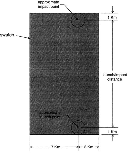
As each comparison system includes a set of DTED Request Algorithms, it is possible that each comparison system may request different portions of DTED. This allows algorithms with specialized DTED requirements to increase or decrease the amount of DTED which must be loaded into main memory. However, most comparison systems use a very basic version of the DTED Request Algorithms. This version requests every block of DTED in a rectangle which encompasses the approximate launch point, the approximate impact points, and a large area surrounding these points called the "swatch". This "swatch" is guaranteed to contain all possible trajectories between the approximate launch and impact points.

(32)

The swatch is a function of the approximate launch and impact locations. The swatch appears as a rectangle whose major axis is oriented in the same direction as the line connecting the approximate launch point to the approximate impact point. The long edge of the swatch is essentially this connecting line extended 1 kilometer on each end (1 kilometer from the approximate launch point extending in the direction away the approximate impact point, and 1 kilometer from the approximate impact point extending in the direction away from the approximate launch point). The short side of the swatch rectangle lies perpendicular to the long edge and extends 3 kilometers in the positive crossrange direction (to the right looking from the approximate launch point to the approximate impact point) and 7 kilometers in the negative crossrange direction (to the left of the launch-impact segment). The swatch is larger to the left of the launch/impact line than to the right because the direction of the projectile's spin causes it to veer to the right during flight. Thus projectiles are launched at an azimuth to the left of the impact point line and allowed to veer back to the right to their intended impact point. The swatch is pictured in Figure 5.

approximate impact point 1 Km swatch launch/impact launch/impact distance 1 Km

T

S7 Km --- - 3 Km

--Figure 5. Swatch encompassing all possible ballistic trajectories

(33)

V-The DTED Request Algorithm first computes the swatch, and then determines the identifiers of all DTED blocks which lie either totally or partially within the area defined by the swatch (as shown in Figure 6). This list of identifiers is then sent to the DTED Controller as the DTED request.

Figure 6. Block selection based on a swatch 3.2.2. DTED Controller

The DTED Controller is responsible for accepting the DTED request from the DTED Request Algorithms and loading the specified blocks into main memory. The DTED Controller also performs, as it reformats the data from DTED file format into blocks, a limited analysis of the data. This analysis is limited to what can be done in a single pass over the data. No iteration may be performed. This single pass corresponds to the single pass which is made as the DTED controller system transfers the data from the DTED files to main memory. Unlike the other components of a comparison system, this subsystem has no timing or memory requirements. The time and memory used by this system is not monitored, and therefore counts in no way towards the analysis or evaluation of the comparison system.

3.2.2.1. Justification for Block Organization of DTED

The purpose of the DTED Controller is to load blocks of DTED into main memory. Each block of DTED covers an area 180 arcseconds by 180 arcseconds. Each block also contains indexing and overhead information which describes the shape and location of the block as well as the organization of the DTED within the block. Each block also contains information specific to the block which may be useful for certain optimizations. The conversion from the original DTED format to the block format requires time and memory. However, this reformatting is a necessary procedure. The reasons for introduction of the block organization strategy are described below.

33 -···-a···-··*···.···c···~·· -- ···-r·-·--i-·- -·-r--··-··- ·- ·i·-·-r--··-··-··-·-r--··-··-·C·-· ··· -·-r--··-··-- ··· · ··· ···· ·~··i···2-'·'~·-1~··· ·-·- · ·i ·· ·--x·xr--···· ·-· ·r··· -x~'-x~~~x-*?ix""~x"~^rxr ·- ··d··-·--·I--··-i-····-

(34)

-·---C---r--·"---The DTED is originally stored on Compact Disc in the 1 degree by 1 degree cells which are described in the military specification for DTED [MIL89]. A single cell of level 2 DTED can contain as many as 12,967,201 elevation posts which requires 24.7 megabytes of memory (as each elevation post consists of a two byte integer). A cell can cover an area as large as 111.3 kilometers by 111.3 kilometers, so in the best case, the entire swatch will be contained within a single cell. Even if only one cell is needed, this may still require 24.7 megabytes of memory which far exceeds the 4 megabytes allowed for storage of data. Since the DTED cells are non-overlapping, in the worst case, a swatch may lie on the intersection of four separate cells which would require nearly 100 megabytes of memory which is certainly unavailable. Furthermore, four cells of DTED would cover nearly 50,000 square kilometers. This is far more than is needed.

The swatch described in Section 3.2.1 encompasses all the DTED which could possibly be needed by a comparison system. As stated previously, the approximate launch and impact locations may only be separated by at most 50 kilometers. This means that the largest swatch possible covers 10 by 52 kilometers or 520 square kilometers.

These facts all seem to indicate that the original storage format of the DTED is intractable for this system. A more reasonable approach is to organize the DTED into uniformly sized blocks which are substantially smaller than the original DTED cells. It has not been shown that a block organization is optimal, but other concepts have been considered and discarded. An alternate concept such as organizing the DTED into rows or columns is made difficult by the fact that the resolution of DTED may change across cell boundaries in both the latitude and longitude directions. Another alternate concept such as storing each elevation post individually is considered to be a special case of uniformly sized blocks with a size of 1 by 1. Thus for the purposes of this project, the DTED will be organized into uniformly sized blocks.

3.2.2.2. Selection of Block Size

As the surface of the earth is the surface of a sphere, there are two methods in which to measure areas on the surface: square kilometers or square arcseconds. The DTED is organized along the lines of the WGS 84 Geodetic Coordinate System which uses angular units. The result is that a square kilometer encompasses different numbers of elevation posts depending on where on the earth the square kilometer is located. A square arcsecond, on the other hand, will always encompass the same number of elevation posts regardless of location (except for variation in DTED resolution due to the latitudinal zones). Furthermore, the surface of the earth cannot be evenly tiled with square kilometers while this is not a problem with square arcseconds. For these reasons, the size of the DTED blocks will be measured in arcseconds of latitude by arcseconds of longitude.

In selecting a block size, it is optimal to choose the largest size possible while still remaining within the memory limits allowed for DTED storage. The larger block size decreases the amount of indexing information because this information is stored on a per block basis. However, a block size which is too large will result in excess unneeded data being carried piggyback by the DTED which is actually needed (as was shown to be the case with the original 1 degree by 1 degree cells). Furthermore, the shape of blocks should be roughly square as this also decreases the total amount of overhead needed.