Comparison and optimization of control policies in automobile manufacturing systems by simulation

(1)

Comparison and optimization of control policies in

automobile manufacturing systems by simulation

by

Chiwon Kim

B.S., Mechanical Engineering

Seoul National University, Republic of Korea, 2002 Submitted to the Department of Mechanical Engineering in partial fulfillment of the requirements for the degree of

Master of Science in Mechanical Engineering at the

MASSACHUSETTS INSTITUTE OF TECHNOLOGY June 2004

c

Author . . . . Department of Mechanical Engineering

May 7, 2004

Certified by . . . . Stanley B. Gershwin Senior Research Scientist, Department of Mechanical Engineering Thesis Supervisor

Accepted by . . . . Ain A. Sonin Chairman, Department Committee on Graduate Students

(2)

(3)

Comparison and optimization of control policies in automobile manufacturing systems by simulation

by Chiwon Kim

Submitted to the Department of Mechanical Engineering on May 7, 2004, in partial fulfillment of the

requirements for the degree of

Master of Science in Mechanical Engineering

Abstract

This thesis studies material flow control policies for automobile manufacturing systems. Various control policies are implemented in simulations of manufacturing systems to test whether they increase the efficiencies of the systems in terms of specific performance mea-sures of interest. Among the control policies, Control Point Policy (CPP) is deeply studied, because this policy is designed for controlling complex manufacturing system with multiple product types.

First, fundamental research in CPP is presented to understand the effects of the pa-rameters on single product type manufacturing systems. Then, multiple product type, assembly-disassembly systems are studied with various control policies, including hybrid policies. Finally, a real automobile manufacturing system case study is presented, and var-ious control policies are experimented on in the simulation model. Because the evaluations of performances are done by simulations, the speed of simulation becomes a very impor-tant problem. This thesis therefore presents a new approach to accelerating the speed of simulation.

Thesis Supervisor: Stanley B. Gershwin

(4)

(5)

Acknowledgments

I would like to thank my advisor, Dr. Stanley Gershwin, for his inspiration, guidance and support throughout the duration of my stay at MIT. I would also like to thank Dr. Alain Patchong for the support in PSA research center. Thanks also go to my colleagues, Youngjae Jang, Jongyoon Kim, Zhenyu Zhang, and Ketty Tanizar. In addition, special thanks to Giha Hyun, and the members of Club4.3. Most of all, the unlimited support from my parents enables me to be what I am now.

(6)

(7)

List of Figures

2-1 Serial Line Model . . . 22

2-2 CP1, DD1, Each . . . 28 2-3 CP1, DD1, Total . . . 28 2-4 CP1, DD2, Each . . . 30 2-5 CP1, DD2, Total . . . 30 2-6 CP2, DD1, Each . . . 31 2-7 CP2, DD1, Total . . . 31 2-8 CP2, DD2, Each . . . 33 2-9 CP2, DD2, Total . . . 33 2-10 CP12, DD1, Each . . . 34 2-11 CP12, DD1, Total . . . 35 2-12 CP12, DD2, Each . . . 35 2-13 CP12, DD2, Total . . . 36

2-14 Two Different Policies . . . 37

2-15 Control Point 1, Due date schemes 1 and 2 . . . 39

2-16 Control Point 2, Due date schemes 1 and 2 . . . 40

2-17 Control Point 1, 2, Due date schemes 1 and 2 . . . 40

2-18 Due Date Scheme 1, all results . . . 41

2-19 Due Date Scheme 2, all results . . . 42

3-1 Multiple parts type manufacturing system . . . 46

3-2 Effect of BBS assumption on Static Priority . . . 47

3-3 Earliest Due Date Policy applied to the model . . . 49

3-4 CONWIP Policy applied to the model . . . 51

(12)

3-6 CONWIP Policy with Static Priority WIP-PR tradeoff curve . . . 53

3-7 CONWIP Policy with EDD using DD2 . . . 54

3-8 CONWIP Policy with EDD using DD2 WIP-PR tradeoff curve . . . 54

3-9 Control Point Policy applied to the model . . . 55

3-10 Control Point Policy with DD2 and Static Priority . . . 57

3-11 Control Point Policy with DD2, SP; WIP-PR tradeoff curve . . . 57

3-12 Modified Control Point Policy applied to the model . . . 58

3-13 Control Point Policy with EDD (DD2) . . . 60

3-14 Control Point Policy with EDD (DD2); WIP-PR tradeoff curve . . . 60

3-15 Hybrid CPP/CONWIP applied to the model . . . 62

3-16 Hybrid CPP/CONWIP with Static Priority and Takt=1.4 . . . 63

3-17 Hybrid CPP/CONWIP with Static Priority and Takt=1.4; WIP-PR tradeoff curve . . . 63

3-18 Hybrid CPP/CONWIP with Static Priority and Takt=2.4 . . . 64

3-19 Hybrid CPP/CONWIP with Static Priority and Takt=2.4; WIP-PR tradeoff curve . . . 64

3-20 Hybrid CPP/CONWIP with Dynamic Priority and Takt=1.4 . . . 65

3-21 Hybrid CPP/CONWIP with Dynamic Priority and Takt=1.4; WIP-PR trade-off curve . . . 66

3-22 Hybrid CPP/CONWIP with Dynamic Priority and Takt=2.4 . . . 67

3-23 Hybrid CPP/CONWIP with Dynamic Priority and Takt=2.4; WIP-PR trade-off curve . . . 67

4-1 Typical Manufacturing System . . . 72

4-2 Manufacturing system to be modified . . . 73

4-3 Manufacturing System with two assembly lines . . . 76

4-4 Substitution Scheme for Assembly Lines . . . 77

4-5 Substitute Machine for Assembly Line . . . 78

4-6 A sample path of random events in assembly line and main line . . . 79

4-7 Markov process model for the simplified assembly system . . . 80

4-8 Embedded Markov chain model for the simplified assembly system . . . 81

(13)

4-10 The simplified model . . . 84

4-11 Exponential two machine one buffer model . . . 85

4-12 Substitution Scheme for Main Lines . . . 85

5-1 PSA Aulnay Factory Layout . . . 90

5-2 The Body Shop Layout . . . 91

5-3 The Body Shop Simulation Model . . . 94

(14)

(15)

List of Tables

2.1 Machine Parameters . . . 22

2.2 Design of simulation experiments: Parameters . . . 25

2.3 Design of simulation experiments: Hedging times . . . 25

2.4 Design of simulation experiments for Hedging times in Control Points 1 and 2 26 2.5 CP1 HT = 80, Due Date Scheme 1, Expected CT = 100 . . . 26

2.6 CP1 HT = 80, Due Date Scheme 2, Takt = 1.25 . . . 27

2.7 CP2 HT = 80, Due Date Scheme 1, Expected CT = 100 . . . 27

2.8 CP2 HT = 80, Due Date Scheme 2, Takt = 1.25 . . . 29

2.9 HT1 = 80, HT2 = 40, Due Date Scheme 1, Expected CT = 100 . . . 29

2.10 HT1 = 80, HT2 = 40, Due Date Scheme 2, Takt = 1.25 . . . 32

3.1 Machine Parameters . . . 46

3.2 Static Priority Results . . . 48

3.3 EDD with due date scheme 1 results . . . 50

3.4 EDD with due date scheme 2 results . . . 50

4.1 Parameters for the simulation . . . 84

4.2 Simulation Results . . . 84

5.1 The body shop performance when policy unchanged . . . 99

5.2 The body shop performance when policy unchanged without pauses and MEF processing stations in the system . . . 99

5.3 CONWIP policy results for the body shop . . . 100

5.4 Samples of token based CPP simulation results . . . 101

(16)

(17)

Chapter 1

Introduction

1.1 Objectives and overview

The efficiency of its manufacturing systems is usually one of the most important concerns of any company. There has been active research on the control of material flow in manufac-turing systems, which has led to several well-known control policies such as MRP, Kanban, and CONWIP. Recently, a new control policy named Control Point Policy (CPP) was de-veloped, which is a method for real-time decision-making in production systems and is derived using dynamic programming. One of the goals of this thesis is to find a systematic way to determine the values of optimal parameters in CPP as well as to develop a method to predict overall performance of the manufacturing systems as parameters vary, by using dynamic discrete-event simulation.

This thesis investigates the requirements of a good control policy in the environment of multiple product types, which is common in automobile companies. Robustness, balancing, and ease of optimization are studied. New control policies such as a hybrid of CPP and CONWIP are suggested. Since the speed of simulation is important, a general approach is developed to simplify the model of a portion of a manufacturing system. The simula-tion with this simplificasimula-tion is much faster and is accurate. Finally, a case study of PSA Peugeot Citro¨en, a French automobile company, is presented, and control of one of PSA’s manufacturing systems is investigated based on the research presented in this thesis.

(18)

1.2 Literature Review

Analytical methods to predict the performances of manufacturing systems can be found in [7]. In this book, an analysis of discrete, exponential, and continuous time models are presented. A two-machine, one-buffer line model serves as a building block to analyze general tree structured assembly–disassembly systems. In addition, an extensive review of models and results of the manufacturing flow line literature can be found in [4]. This paper presents exact methods for obtaining quantitative measures of performance for small systems and approximate methods for large systems.

One of the most popular push control policies, Manufacturing Resource Planning (MRP II), is introduced in [10]. This book also describes Material Requirement Planning (MRP), Earliest Due Date (EDD), and Kanban. This book is a extensive reference of the dynamics of manufacturing systems.

The CONWIP control policy, which is one of the most famous pull control policies, is described in [19], [10]. Research on the comparison of pull policies with push policies is presented in [20]. This paper explains the apparent superior performance of pull systems. Another comparison of production line control mechanisms can be found in [2].

The issue of customer service in pull production systems is presented in [18]. This paper also shows that CONWIP not only has better service than a pure kanban system, but also solves certain implementation problems. In addition, [3] shows the performance of the hybrid of CONWIP and the finite buffer policy.

The CPP is introduced in [8]. This paper presents details of CPP with three alternative versions of CPP: time-based, surplus-based, and token-based. The CPP is based on a dynamic programming problem formulation of factory scheduling. An analytical solution to the dynamic programming problem for a simple factory is presented in [21]. Also, simulation experiments of CPP are investigated in [5], [9], and [22]. In particular, [9] is for the single product type manufacturing systems, and [22] is for the multiple product type systems.

Li [14] presents the overlapping decomposition method for the estimation of the produc-tion rate of a complex manufacturing system with assembly, parallel, rework, feed-forward and scrap operations. The idea in this paper is extended in the simulation substitution methodology presented in this thesis.

(19)

Various simulation algorithms, including design of experiment and variance reduction tech-nique can be found in these books.

Kouikoglou and Phillis [12] present the method of acceleration of the simulation by separating major events from minor events. By combining analytical methods for minor events and the discrete event simulations for major events, this book shows that the speed can be improved while the accuracy is acceptable for most purposes.

Many queuing networks models assume that certain random variables are independent and exponentially distributed. In modelling manufacturing systems, it is common to assume that the mean time to failure and the mean time to repair are independent and follow exponential distributions. Inman [11] assesses the validity of two common assumptions regarding the randomness in automobile manufacturing systems with actual data collected from automotive body welding lines.

PSA Aulnay factory, which is the source of the case study in this thesis, is introduced in [16]. This paper treats the improvements of throughput with minimal capital investment and no compromise in quality.

1.3 Thesis Outline

Chapter 2 investigates the relations between parameters in CPP for single product type, serial line manufacturing systems. Chapter 3 treats an extension of the research in Chapter 2 to multiple product types and presents some hybrid control policies in order to include more performance measures such as balancing performance. Chapter 4 studies substitution approaches in order to accelerate the speed of simulation while maintaining the accuracy. Chapter 5 introduces an automobile company case study. Various control policies are im-plemented in a simulation model of the factory.

(20)

(21)

Chapter 2

Parameters in the Control Point

Policy For Single Part Type

This chapter has two purposes. The first is to study a method of getting optimal tradeoffs between performance measures in the Control Point Policy (CPP). The other is to interpret what the parameters of CPP actually mean. A simple serial line model with single part type is explored to study the effects of the parameters. Two different due date assignment schemes are used independently for comparison. The Simul8 discrete event based simulation package is used.

The assessment of the performance of a control policy is a very important issue. In previous research on CPP, it was common to investigate the tradeoff between service level and work in process (WIP). However, in this thesis, production rate is used instead of service level. By using production rate instead of service level, we can eliminate simulation parameters which are related to service level such as a customer arrival rate in the MTO environment. In addition, there is a strong positive correlation between production rate and service level.

2.1 Model Description and Assumption

2.1.1 Serial Line Model

Figure 2-1 shows the model that is studied in this chapter. The model consists of three identical but unsynchronized machines. The parameters of the machines and buffers are in

(22)

RM Buffer

VM1: Due date assignment

VM2: Control Point 1 VM3: Control Point 2

Machine 1 Machine 2 Machine 3

Buffer 0 Buffer 1 Buffer 2 FG buffer

Figure 2-1: Serial Line Model

Table 2.1. There is no bottleneck in the system because of the symmetry. Often engineers try to balance the capacity of each machine in most factories, so it is reasonable to study such models that have no specific bottleneck. Note that a machine in Figure 2-1 can also represent a complex processing station.

Table 2.1: Machine Parameters M1 M2 M3 Processing Time 1 1 1

MTTR 10 10 10

MTTF 90 90 90

In addition, in order to provide variability, the processing time, failure time, and repair time follow the exponential distribution. The small squares in the model represent virtual machines (VM) for the implementation of CPP. These VMs have perfect reliability and zero or deterministic processing times. In particular, VM1’s processing time is zero, so buffer 0 is full all the time. The rule to calculate the processing times of VMs other than VM1 is explained in the following subsections. There are five buffers in the model as follows.

• RM buffer – raw material buffer with unlimited capacity and never starved

• Buffer 0 – capacity of 50 parts waiting for the production

• Work in process buffers 1, 2 – capacities of 50 parts each

(23)

2.1.2 Implementation of CPP

The implementation of the Control Point Policy can be done easily by introducing virtual machines. The first virtual machine assigns the due dates to the parts passing through. The second and the last virtual machines apply the hedging time logic to the parts. In addition, adding and removing control points at the system is equivalent to adding and removing virtual machines.

Hedging time logic The hedging time logic of the single part type CPP can be expressed in the following form.

1. Select the part in the buffer with the earliest due date.

2. Calculate the virtual machine processing time τvm for that part, where

τ = Due date - Simulation running time - Hedging time τvm = |τ |+τ₂

Proof If the part is ready, VM processing time is zero. Thus this part can pass through without delay. If the part is not ready, then just after the VM processing time calculated above, it becomes ready.

2.1.3 Due date Assignment Schemes

Due date assignment scheme 1 (DD1)

Due date = Entry time + Expected cycle time

An expected cycle time is one of the performance measures, but we should estimate it before running the simulation. Thus we can see the expected cycle time as an independent parameter to control, even though the name of this parameter implies something measured. From now on, expected cycle time is an independent parameter of this due date scheme. In a manufacturing system with this due date scheme, a part is assigned a due date that is not related to the state of the system if the expected cycle time is constant. Suppose the production is behind the target production by some random events. The system does not try to catch up the target production because the due date is not related to the state of

(24)

the system, and the capacity is wasted as a result. On the other hand, we have control of the flow if the target production rate is less than the capacity of the system with this due date scheme. Parameters to optimize are hedging times and an expected cycle time. Note that cycle time in this thesis is called lead time in some literature, we use processing time to describe a single machine.

Due date assignment scheme 2 (DD2)

Due date = (Takt time)(Serial number + an offset)

Intuitively, this scheme is favorable in a situation in which explicit target production rate exists. As will be demonstrated, this scheme is much more robust in handling the random events in the system. In contrast to due date scheme 1, this scheme allows catching up with the target production rate, so less of the capacity is wasted. Parameters to optimize are hedging times and the takt time.

2.2 Design of Simulation Experiments

The purpose of this section is to present the design of the simulation experiments using the serial line model. First, the location and the number of control points are considered as follows.

1. Simulation with single control point (CP1) result

2. Simulation with single control point (CP2) result

3. Simulation with multiple control points (CP1,CP2) result

We can get useful insights about the CPP behavior by comparing the single control point simulation results to the results of multiple control points.

2.2.1 Single control point experiments with due date scheme 1

In the first group of simulation experiments, we activate only control point 1 with due date scheme 1. There are two parameters to tune: a hedging time for control point 1 and an expected cycle time for due date scheme 1. There are 10 sets of simulations in this group.

(25)

A set of simulations consists of 25 runs. Each set has different expected lead time values, and each run in a set has different hedging time values. See Table 2.2 and Table 2.3.

In the second group of simulation experiments, we activate only control point 2 with due date scheme 1. The design of the simulation experiments is the same as the first group except that we are using hedging times for control point 2 instead of hedging times for control point 1.

2.2.2 Single control point experiments with due date scheme 2

In the third group of simulation experiments, we activate only control point 1 with due date scheme 2. A takt time and an offset are the parameters to control as well as a hedging time. However, because the offset affects only the duration of the transient period of the system, we can fix it as a constant. Thus there are only two parameters to vary: a takt time and a hedging time. There are 10 sets of simulations in this group and each set consists of 25 runs. Each set has a different takt time, and each run has a different hedging time. These are summarized in Table 2.2 and Table 2.3.

For the experiments of control point 2 with due date scheme 2 as the last group of simulation experiments, the design is the same as the third group except that we are using hedging times for control point 2 instead of hedging times for control point 1.

Table 2.2: Design of simulation experiments: Parameters

Set number 1 2 3 4 5 6 7 8 9 10

Expected CT 0 20 40 60 80 100 120 140 160 180 Takt Time 0.25 0.5 0.75 1 1.25 1.5 1.75 2 2.25 2.5

Table 2.3: Design of simulation experiments: Hedging times

Run number 1 2 3 4 5 6 7 · · · 21 22 23 24 25

Hedging times 0 10 20 30 40 50 60 · · · 200 210 220 230 240

2.2.3 Control Point 1 and 2 experiments

As we decide the values of hedging time 1 and hedging time 2, it is reasonable to assume that hedging time 1 is bigger than hedging time 2. Expected cycle time is used for each

(26)

set of simulations as in Table 2.2 and 2.3 for the due date scheme 1. Similarly, takt time is used for each set of simulations as in Table 2.2 and 2.3 the due date scheme 2. Hedging times are assigned as in Table 2.4 in a set of simulations.

Table 2.4: Design of simulation experiments for Hedging times in Control Points 1 and 2

Run 1 2 3 4 5 6 7 8 9 10 11 12 13 HT1 20 40 40 40 60 60 60 80 80 80 80 100 100 HT2 10 10 20 30 10 30 50 10 30 50 70 10 30 Run 14 15 16 17 18 19 20 21 22 23 24 25 HT1 100 100 100 120 120 120 120 120 120 140 140 140 HT2 50 70 90 10 30 50 70 90 110 30 70 110

2.3 Simulation Results

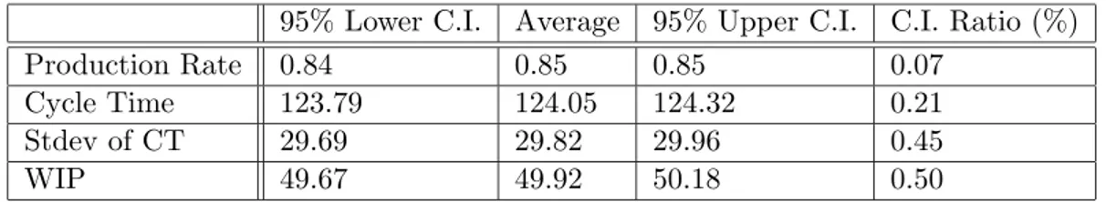
2.3.1 Statistical Validations

This section confirms that the results are statistically acceptable before the actual results of the sets of simulations are presented. The simulation duration of each run in a set is 1,000,000 minutes with warming up period 5,000 minutes. Table 2.5 to 2.10 gives important measures for the reliability of the data. The number of replications to get the confidence intervals is 250. Note that the C.I. ratio is defined as the ratio of the length of confidence interval (95% level) to the magnitude of the measure. For more information of confidence intervals, see [17].

Table 2.5: CP1 HT = 80, Due Date Scheme 1, Expected CT = 100 95% Lower C.I. Average 95% Upper C.I. C.I. Ratio (%)

Production Rate 0.84 0.85 0.85 0.07

Cycle Time 123.79 124.05 124.32 0.21

Stdev of CT 29.69 29.82 29.96 0.45

WIP 49.67 49.92 50.18 0.50

Tables 2.5 - 2.8 show that lengths of confidence intervals are significantly small. The ratios of confidence intervals to the average of performance measures are less than 1%. Therefore, we can trust that the average values of these performance measures are in the

(27)

Table 2.6: CP1 HT = 80, Due Date Scheme 2, Takt = 1.25

95% Lower C.I. Average 95% Upper C.I. C.I. Ratio (%)

Cycle Time 103.45 103.75 104.05 0.29

Stdev of CT 26.30 26.51 26.72 0.79

WIP 28.01 28.28 28.55 0.96

Table 2.7: CP2 HT = 80, Due Date Scheme 1, Expected CT = 100 95% Lower C.I. Average 95% Upper C.I. C.I. Ratio (%)

Cycle Time 123.42 123.69 123.95 0.22

Stdev of CT 29.91 30.04 30.18 0.45

WIP 49.46 49.71 49.97 0.51

steady state of the system.

Tables 2.9 and 2.10 show statistical validations in situations of two control points. These tables give similar information as before, but they contain more information, including the confidence intervals of the standard deviations of the performance measures such as PR and WIP. For example, in Table 2.9, the confidence interval of the standard deviation of WIP is [1.48, 1.77] with confidence interval ratio 11.51%. The C.I. ratio seems rather high in this case, but the length of C.I. are small. This is acceptable because what we are interested in this chapter are the steady state behaviors of the average values of performance measures.

2.3.2 Control Point 1 Simulation Results

Figure 2-2 shows plots of the CP1 simulation results with due date scheme 1. In this figure, each small plot has a different expected cycle time parameter values from Table 2.2. Figure 2-3 shows the plots of all results in a single figure. In other words, all the plots in Figure 2-2 are aggregated in Figure 2-3.

In Figure 2-2, we can see that when expected cycle time is low, the hedging time param-eter does not affect the steady state behavior of the system. Moreover, as expected cycle time increases, the the system gains more control over the tradeoff between the WIP and production rate. However, as shown in Figure 2-3, the set of simulations with the largest

(28)

0.2 0.3 0.4 0.5 0.6 0.7 0.8 0.9 0 10 20 30 40 50 60 Production rate WIP CP1 DD1

Set 1 through 10. Each has 25 runs with different hedging time. Control Point 1 Optimization with Due Date Scheme 1

0.2 0.3 0.4 0.5 0.6 0.7 0.8 0.9 0 10 20 30 40 50 60 Production rate WIP CP1 DD1 0.2 0.3 0.4 0.5 0.6 0.7 0.8 0.9 0 10 20 30 40 50 60 Production rate WIP CP1 DD1 0.2 0.3 0.4 0.5 0.6 0.7 0.8 0.9 0 10 20 30 40 50 60 Production rate WIP CP1 DD1 0.2 0.3 0.4 0.5 0.6 0.7 0.8 0.9 0 10 20 30 40 50 60 Production rate WIP CP1 DD1 0.2 0.3 0.4 0.5 0.6 0.7 0.8 0.9 0 10 20 30 40 50 60 Production rate WIP CP1 DD1 0.2 0.3 0.4 0.5 0.6 0.7 0.8 0.9 0 10 20 30 40 50 60 Production rate WIP CP1 DD1 0.2 0.3 0.4 0.5 0.6 0.7 0.8 0.9 0 10 20 30 40 50 60 Production rate WIP CP1 DD1 0.2 0.3 0.4 0.5 0.6 0.7 0.8 0.9 0 10 20 30 40 50 60 Production rate WIP CP1 DD1 0.2 0.3 0.4 0.5 0.6 0.7 0.8 0.9 0 10 20 30 40 50 60 Production rate WIP CP1 DD1 Figure 2-2: CP1, DD1, Each 0.2 0.3 0.4 0.5 0.6 0.7 0.8 0.9 1 0 10 20 30 40 50 60 Production rate WIP CP1 DD1 Figure 2-3: CP1, DD1, Total

(29)

Table 2.8: CP2 HT = 80, Due Date Scheme 2, Takt = 1.25

95% Lower C.I. Average 95% Upper C.I. C.I. Ratio (%)

Cycle Time 130.82 131.00 131.17 0.13

Stdev of CT 25.55 25.69 25.84 0.57

WIP 49.87 50.09 50.31 0.44

Table 2.9: HT1 = 80, HT2 = 40, Due Date Scheme 1, Expected CT = 100 95% Lower C.I. Average 95% Upper C.I. C.I. Ratio (%)

Production Rate 0.84 0.84 0.84 0.07 Stdev of PR 0.00 0.00 0.00 10.82 Cycle Time 125.26 125.52 125.78 0.21 Stdev of CT 29.55 29.68 29.81 0.45 WIP 49.87 50.11 50.36 0.49 Stdev of WIP 1.48 1.67 1.77 11.51 Buffer 1 28.99 29.11 29.23 0.42 Buffer 2 20.88 21.01 21.13 0.59 Stdev of Buffer 1 0.87 0.98 1.04 11.32 Stdev of Buffer 2 0.89 1.01 1.05 11.51

expected cycle time is a superset of all the other sets.

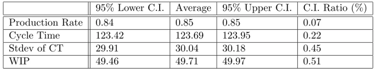
Figure 2-4 and 2-5 have similar structures as Figure 2-2 and 2-3. Figure 2-4 shows each plot of CP1 simulation results with due date scheme 2. In Figure 2-4, each small plot has a different takt time as in Table 2.2. Also, Figure 2-5 shows the plots of all results of Figure 2-4 in the same graph.

An important observation is that the hedging time parameter does not make any differ-ence in the steady state behavior of the system in due date scheme 2. Only the takt time parameter affects the tradeoff between WIP and production rate. In this sense, we can say that the control policy with due date scheme 2 is less sensitive to the internal states of the system.

2.3.3 Control Point 2 Simulation Results

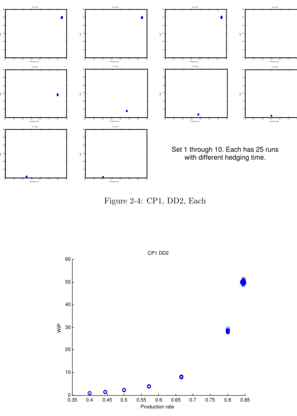
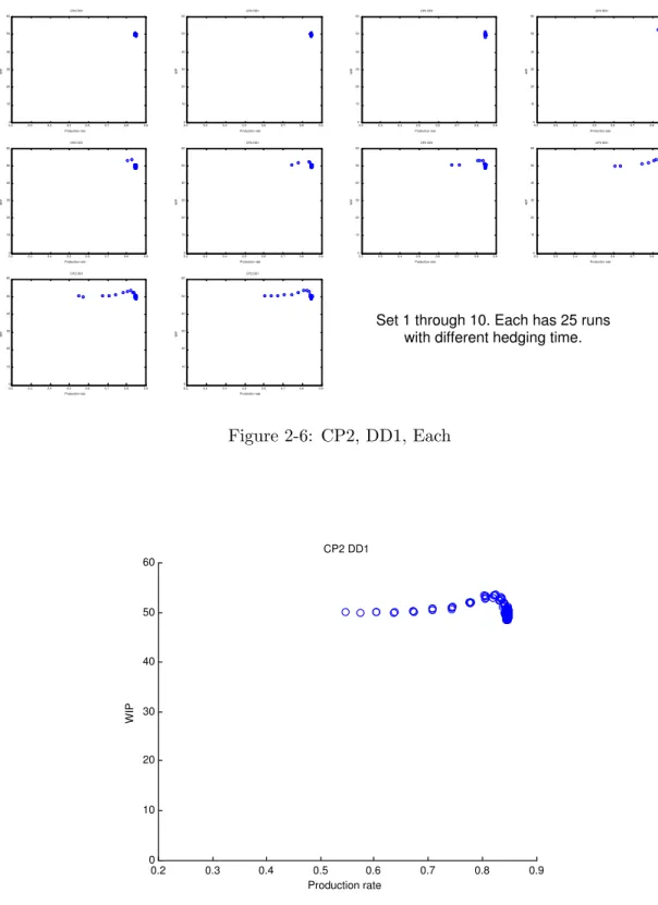
Figure 2-6 and 2-7 show the results for the group of simulations activating control point 2 with due date scheme 1. The structures of the figures are the same as previous section.

(30)

0.2 0.3 0.4 0.5 0.6 0.7 0.8 0.9 0 10 20 30 40 50 60 Production rate WIP CP1 DD2 0.2 0.3 0.4 0.5 0.6 0.7 0.8 0.9 0 10 20 30 40 50 60 Production rate WIP CP1 DD2 0.2 0.3 0.4 0.5 0.6 0.7 0.8 0.9 0 10 20 30 40 50 60 Production rate WIP CP1 DD2 0.2 0.3 0.4 0.5 0.6 0.7 0.8 0.9 0 10 20 30 40 50 60 Production rate WIP CP1 DD2 0.2 0.3 0.4 0.5 0.6 0.7 0.8 0.9 0 10 20 30 40 50 60 Production rate WIP CP1 DD2 0.2 0.3 0.4 0.5 0.6 0.7 0.8 0.9 0 10 20 30 40 50 60 Production rate WIP CP1 DD2 0.2 0.3 0.4 0.5 0.6 0.7 0.8 0.9 0 10 20 30 40 50 60 Production rate WIP CP1 DD2 0.2 0.3 0.4 0.5 0.6 0.7 0.8 0.9 0 10 20 30 40 50 60 Production rate WIP CP1 DD2 0.2 0.3 0.4 0.5 0.6 0.7 0.8 0.9 0 10 20 30 40 50 60 Production rate WIP CP1 DD2 0.2 0.3 0.4 0.5 0.6 0.7 0.8 0.9 0 10 20 30 40 50 60 Production rate WIP CP1 DD2

Figure 2-4: CP1, DD2, Each 0.350 0.4 0.45 0.5 0.55 0.6 0.65 0.7 0.75 0.8 0.85 10 20 30 40 50 60 Production rate WIP CP1 DD2 Figure 2-5: CP1, DD2, Total

(31)

Figure 2-6: CP2, DD1, Each 0.2 0.3 0.4 0.5 0.6 0.7 0.8 0.9 0 10 20 30 40 50 60 Production rate WIP CP2 DD1 Figure 2-7: CP2, DD1, Total

(32)

Table 2.10: HT1 = 80, HT2 = 40, Due Date Scheme 2, Takt = 1.25 95% Lower C.I. Average 95% Upper C.I. C.I. Ratio (%)

Production Rate 0.80 0.80 0.80 0.01 Stdev of PR 0.00 0.00 0.00 15.09 Cycle Time 121.50 121.70 121.90 0.17 Stdev of CT 24.46 24.63 24.80 0.68 WIP 41.54 41.73 41.93 0.47 Stdev of WIP 1.12 1.28 1.35 12.56 Buffer 1 28.99 29.08 29.17 0.30 Buffer 2 12.54 12.65 12.76 0.88 Stdev of Buffer 1 0.62 0.70 0.74 10.66 Stdev of Buffer 2 0.80 0.90 0.94 10.92

expected cycle time is low, the hedging time parameter does not affect the steady state behavior of the system. The system gains more control over the tradeoff between the WIP and production rate as the expected cycle time increases. Figure 2-7 shows that the set of simulations with the largest expected cycle time is a superset of all the other sets.

There is no tradeoff between the WIP and production rate in Figure 2-7. Rather, there exists explicitly the best WIP level and production rate, which is the rightmost point. The overshoot is because WIP is piling up in front of the control point, which prevents parts to pass due to the control logic.

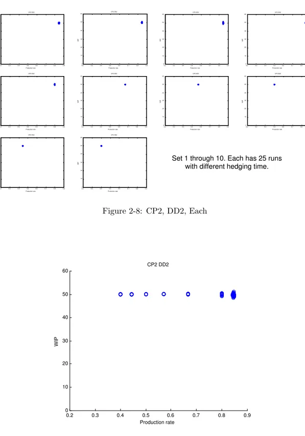
Figure 2-8 shows each plot of CP2 simulation results with due date scheme 2. Figure 2-9 shows aggregated plots of all results in a single figure.

As in the previous section, hedging time parameter does not make any differences in the steady state behavior of the system with due date scheme 2. Only takt time parameter affects the tradeoff between WIP and production rate. Again due date scheme 2 seems more robust to the internal states of the system. In addition, there is no change in WIP as parameters vary in Figure 2-9. Thus there exists explicit optimal set of parameters which gives us the largest production rate.

2.3.4 Control Point 1 and 2 Simulation Results

Figure 2-10 and 2-11 show the results for the group of simulations activating both the control point 1 and control point 2 with due date scheme 1. The structures of the figures

(33)

Figure 2-8: CP2, DD2, Each 0.2 0.3 0.4 0.5 0.6 0.7 0.8 0.9 0 10 20 30 40 50 60 Production rate WIP CP2 DD2 Figure 2-9: CP2, DD2, Total

(34)

0.2 0.3 0.4 0.5 0.6 0.7 0.8 0.9 0 10 20 30 40 50 60 Production rate WIP CP 12 DD1 0.2 0.3 0.4 0.5 0.6 0.7 0.8 0.9 0 10 20 30 40 50 60 Production rate WIP CP 12 DD1 0.2 0.3 0.4 0.5 0.6 0.7 0.8 0.9 0 10 20 30 40 50 60 Production rate WIP CP 12 DD1 0.2 0.3 0.4 0.5 0.6 0.7 0.8 0.9 0 10 20 30 40 50 60 Production rate WIP CP 12 DD1 0.2 0.3 0.4 0.5 0.6 0.7 0.8 0.9 0 10 20 30 40 50 60 Production rate WIP CP 12 DD1 0.2 0.3 0.4 0.5 0.6 0.7 0.8 0.9 0 10 20 30 40 50 60 Production rate WIP CP 12 DD1 0.2 0.3 0.4 0.5 0.6 0.7 0.8 0.9 0 10 20 30 40 50 60 Production rate WIP CP 12 DD1 0.2 0.3 0.4 0.5 0.6 0.7 0.8 0.9 0 10 20 30 40 50 60 Production rate WIP CP 12 DD1 0.2 0.3 0.4 0.5 0.6 0.7 0.8 0.9 0 10 20 30 40 50 60 Production rate WIP CP 12 DD1 0.2 0.3 0.4 0.5 0.6 0.7 0.8 0.9 0 10 20 30 40 50 60 Production rate WIP CP 12 DD1

Set 1 through 10. Each has 25 runs with different hedging time. Control Point 1, 2 Optimization with Due Date Scheme 1

Figure 2-10: CP12, DD1, Each

are the same as in previous sections.

As we can see in Figure 2-10, when the expected cycle time is small, hedging times do not affect the behavior of the system. As the expected cycle time increases, the steady state behavior of the system has wider range of tradeoff between WIP and production rate. Furthermore, the scattered data is bounded with the boundary of the convex hull of the scattered data. We can separate the boundary into a concave part and a convex part. The relation of the convex boundary and the single control point results is suggested in the following section. Actually, it turns out that the convex part of the boundary is almost the same as the curve of the single control point cases.

In the sets using larger expected cycle times, what approximately determines the pro-duction rate is the hedging time of control point 1, while what determines the WIP level is the difference between the hedging times for the control points. As hedging time difference gets smaller, the lower WIP is observed. If the difference is big, the trajectory is similar to that of single control point 2 with due date scheme 1.

Figure 2-12 shows each plot of CP1 and CP2 simulation results with due date scheme 2. Figure 2-13 shows an aggregated plot of all results.

(35)

0.2 0.3 0.4 0.5 0.6 0.7 0.8 0.9 0 10 20 30 40 50 60 Production rate WIP CP 12 DD1 Figure 2-11: CP12, DD1, Total 0.2 0.3 0.4 0.5 0.6 0.7 0.8 0.9 0 10 20 30 40 50 60 Production rate WIP CP 12 DD2 0.2 0.3 0.4 0.5 0.6 0.7 0.8 0.9 0 10 20 30 40 50 60 Production rate WIP CP 12 DD2 0.2 0.3 0.4 0.5 0.6 0.7 0.8 0.9 0 10 20 30 40 50 60 Production rate WIP CP 12 DD2 0.2 0.3 0.4 0.5 0.6 0.7 0.8 0.9 0 10 20 30 40 50 60 Production rate WIP CP 12 DD2 0.2 0.3 0.4 0.5 0.6 0.7 0.8 0.9 0 10 20 30 40 50 60 Production rate WIP CP 12 DD2 0.2 0.3 0.4 0.5 0.6 0.7 0.8 0.9 0 10 20 30 40 50 60 Production rate WIP CP 12 DD2 0.2 0.3 0.4 0.5 0.6 0.7 0.8 0.9 0 10 20 30 40 50 60 Production rate WIP CP 12 DD2 0.2 0.3 0.4 0.5 0.6 0.7 0.8 0.9 0 10 20 30 40 50 60 Production rate WIP CP 12 DD2 0.2 0.3 0.4 0.5 0.6 0.7 0.8 0.9 0 10 20 30 40 50 60 Production rate WIP CP 12 DD2 0.2 0.3 0.4 0.5 0.6 0.7 0.8 0.9 0 10 20 30 40 50 60 Production rate WIP CP 12 DD2

Set 1 through 10. Each has 25 runs with different hedging time. Control Point 1, 2 Optimization with Due Date Scheme 2

(36)

0.2 0.3 0.4 0.5 0.6 0.7 0.8 0.9 0 10 20 30 40 50 60 Production rate WIP CP 12 DD2 Figure 2-13: CP12, DD2, Total

In due date scheme 2 with both of the control points, the tendency is more explicit. The convex hull of the scattered data can be obtained, as in due date scheme 1, which turn out that the same shapes as single control point cases. What determines the production rate is takt time, while what determines the WIP level is the difference between the hedging times. The smaller the difference, the lower the WIP level. If the difference is big, then the trajectory is similar to that of single control point 2 with due date scheme 2.

2.4 Interpretations

In this section, the results of previous section are interpreted, and the due date schemes are analyzed and compared. This section is completed by representing insights from the simulation experiments of the Control Point Policy.

2.4.1 Criteria of a good policy

There are several requirements for a good control policy. Though the criteria of a good policy are restricted to single part type manufacturing systems in this chapter, the requirements below are quite general.

(37)

Production Rate WIP

0 1

Optimal Control Tradeoff Curves

Control Policy A

Control Policy B

Figure 2-14: Two Different Policies

An optimal performance curve can be obtained by the boundary of convex hull of the data from many sets of simulations. For example, in Figure 2-11, we can get an approximately optimal curve from the convex part of the boundary of the convex hull. Optimal performance curves of two different policies, which are operated with optimal parameter values, are shown in Figure 2-14. Control policy B is a better policy than control policy A because control policy B has lower level of inventory for each value of the production rate. Furthermore, the average queuing time in the system is lower in control policy B than control policy A from Little’s Law ([6]).

• Robustness and Sensitivity

The policy should be robust to the random events of the system. For example, if a machine failure occurs, a better policy will somehow compensate for the bad effects of the failure. On the other hand, a good policy should be sensitive to the parameters of the policy. For example, in the due date scheme 2 as Figure 2-5, the hedging time parameter has no role in the control policy. In this case, we can get rid of the hedging time parameter from the policy itself.

• Ease of optimization

Generally, the optimization of a control policy is difficult and time-consuming. Even though a company uses a very fast simulation model of a manufacturing system, the number of simulation experiments to find the optimal set of parameters grows

(38)

exponentially in the number of parameters. Therefore, to find the optimal parameters, the number of parameter should be small.

• Ease of implementation

The implementation of the policy should be easy. For example, the implementation of multiple control points would be more complex than the implementation of a single control point. In principle, the implementation of control policy should not involve any actual change in the machines for ease of implementation of a control policy.

2.4.2 Capacity and target production rate

The capacity of the model can be obtained by running the simulation without any control logic. The capacity of the model is 0.85 parts/min, and at that capacity, the average WIP is 50. In due date scheme 1, expected cycle time determines the target production rate for the system. From the Little’s law, low expected cycle time means higher production rate while keeping the average inventory constant. Also, in due date scheme 2, the takt time parameter directly determines the target production rate.

Intuitively, if the target production rate is greater than the capacity, then the system should be at its capacity point. In case of the simulation sets 1 through 4, where the expected cycle time and takt time are lower than or equal to 40 and 1 respectively, the target production rate is greater than the capacity. Therefore, as in Figures 2-2, 2-4, 2-6, 2-8, 2-10 and 2-12, the first four small plots just have one big aggregated point each, which is actually 25 points with different hedging time values.

As a conclusion, if the target production rate is greater than capacity, control logic becomes less useful. Note that this is not a disadvantage of that control policy. Rather, a bad control policy will remain effective and reduce the flow to less than capacity even though the target production rate is greater than the capacity.

2.4.3 Due date assignment scheme comparison

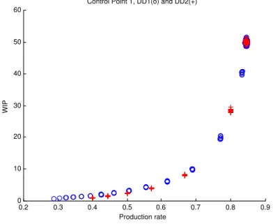
Figure 2-15 shows all the simulation results which makes use of only Control Point 1. In other words, it is a figure that Figures 2-3 and 2-5 are added. Similarly, Figure 2-16 shows all the simulation results of single control point 2 regardless of due date schemes. Therefore, it is a figure that Figures 2-7 and 2-9 are added. Finally, Figure 2-17 is for the simulation

(39)

0.2 0.3 0.4 0.5 0.6 0.7 0.8 0.9 0 10 20 30 40 50 60

Control Point 1, DD1(o) and DD2(+)

Production rate

WIP

Figure 2-15: Control Point 1, Due date schemes 1 and 2

results of both control points utilization, which is a figure that Figures 2-11 and 2-13 are added. A circle is used for each data point from due date scheme 1, while a plus sign is used for each data point from due date scheme 2.

In Figure 2-15, the curve of due date scheme 2 is only slightly lower than, or almost the same as the curve of due date scheme 1. Therefore the first criterion of Section 2.4.1 cannot be applied. In terms of robustness, due date scheme 2 is better, because it is not affected by the hedging time parameters. Furthermore, there is no reason to keep a hedging time parameter as a parameter for the control policy because due date scheme 2 is not sensitive to the control parameter at all. Therefore, due date scheme 2 has only a single parameter that is a takt time parameter, while due date scheme 1 has a expected cycle time and hedging time parameters. Thus, due date scheme 2 is a better policy in terms of ease of optimization.

In Figure 2-16, the optimal parameter sets are explicit, and they are coincident with each other. Further, the optimal parameter set gives the same performance as when there is no control logic. In Figure 2-17, two results from each due date scheme share almost the same region. Therefore the abilities of two due date schemes with two control points are almost the same.

(40)

0.2 0.3 0.4 0.5 0.6 0.7 0.8 0.9 0 10 20 30 40 50 60

Control Point 2, DD1(o) and DD2(+)

Production rate

WIP

Figure 2-16: Control Point 2, Due date schemes 1 and 2

0.2 0.3 0.4 0.5 0.6 0.7 0.8 0.9 0 10 20 30 40 50 60

Control Point 1 and 2, DD1(o) and DD2(+)

Production rate

WIP

(41)

0.2 0.3 0.4 0.5 0.6 0.7 0.8 0.9 0 10 20 30 40 50 60

Due Date Assignment Scheme 1, CP1(o), CP2(triangles), CP1 and CP2(+)

Production rate

WIP

Figure 2-18: Due Date Scheme 1, all results

2.4.4 Control Point Locations and Policy Performance

Figure 2-18 aggregates all the simulation results done with due date scheme 1. In other words, it is a figure that Figures 2-3, 2-7, and 2-11 are added. Similarly, Figure 2-19 aggregates all the simulation results done with due date scheme 2. Thus Figure 2-19 is a figure that Figures 2-5, 2-9, and 2-13 are added. Control point 1 results are marked with circles, and control point 2 results are marked with triangles, while two-control-point results are marked with pluses.

As in the Figures 2-18 and 2-19, the results of control point 1 simulation experiments serve as a lower bound of the region covered by the results from both of the control points. At the same time, the results of control point 2 simulation experiments serve as a upper bound of the region covered by the results from two control points.

As a conclusion, the locations of control points are important. Furthermore, control point 1 is enough for the best performance of CPP implemented into the single part type, serial line manufacturing systems.

(42)

0.2 0.3 0.4 0.5 0.6 0.7 0.8 0.9 0 10 20 30 40 50 60

Due Date Assignment Scheme 2, CP1(o), CP2(triangles), CP1 and CP2(+)

Production rate

WIP

Figure 2-19: Due Date Scheme 2, all results

2.5 Conclusions and Insights

2.5.1 Summary

In this chapter, a single part type, serial line manufacturing system simulation model is developed and tested. The implementation of the Control Point Policy into a simulation is done easily by introducing virtual machines. Two different due date assignment schemes are explored. Each due date assignment scheme and the CPP control logic have parameters such as expected cycle time, takt time, and hedging times. Sets of simulations are designed and the results are collected. Confidence intervals for the results are obtained for several sets of simulations.

2.5.2 Conclusions and Insights

The following is the conclusions to this chapter. Note that the conclusions are confined to the single part type, serial line manufacturing systems.

• If the target production rate is higher than the capacity, a good control policy should behave like a simple push policy. The Control Point Policy has this property.

(43)

steady state behavior of the system only when the target production rate is smaller than capacity.

• In due date scheme 2 with a single control point, hedging time has no meaning. Therefore we can modify the policy so that hedging time is no longer a parameter. Then the policy becomes easier to optimize.

• If both control points are activated, and the target production rate is less than the capacity, the difference between the hedging times affects the steady state behavior of the system. If the gap is small, then the behavior approaches that of the case in which only control point 1 is activated. On the other hand, if the gap is large, then the behavior approaches that of the case in which only control point 2 is activated.

• The location of control points is one of the most important factors that affects the performance of the control. Single control point 1 shows best performance than any other combination.

Finally, we can get some insights from the conclusions above.

• The hedging time parameter has its meaning only in some special cases.

• It is better to use only single control point. This provides the best performance, and it is easiest to optimize and implement.

• It is better to put the control point as far upstream as possible.

• Due date scheme 2 is potentially better in terms of robustness and ease of optimization, because we can have one fewer parameter.

(44)

(45)

Chapter 3

Comparison of control policies for

two part types

In this chapter, a two part type manufacturing system is explored. In particular, each part type shares one resource which is a machine or a processing station. Various control policies are applied to this system, and compared. The goal of this chapter is to see the behaviors of this system. By using this system as an example, we can get useful and practical insights for lager scale multiple part type manufacturing systems.

The main performance measures are production rate, average level of work in pro-cess(WIP), and cycle time. In the multiple part type manufacturing environment, it is often important to balance the flows between two part types. For example, in some auto-mobile manufacturing systems, there is no preference between models, and any model can not be less important because of marketing reasons. Therefore the degree of unbalance is included as one of performance measures. The definition of the degree of unbalance in this chapter is defined as

|P rA− P rB|

P rA+ P rB

where P rA is the production rate of part type A, and P rB is the production rate of part

(46)

Part Type A Part Type B Machine A1 Machine A3 Machine B1 Machine B3 Machine 2 Buffer A1 Buffer A2 Buffer B1 Buffer B2 RM Buffer RM Buffer FG Buffer FG Buffer

Figure 3-1: Multiple parts type manufacturing system

3.1 Model description

Figure 3-1 is the basic model that is investigated with several control policies. Table 3.1 shows the parameters of the machines in the model. Each processing time, MTTR, and MTTF follows an exponential distribution. RM buffers are raw material buffers and they are never starved by assumption. Also, FG buffers are finished goods buffers for each part type. FG buffers are never blocked. Every other buffer has finite capacity of 25.

Table 3.1: Machine Parameters

M-A1 M-B1 M2 M-A3 M-B3

Processing Time 2 2 1 2 2

MTTR 10 10 10 10 10

MTTF 90 90 90 90 90

The machine 2 (M2) should make decision which part to load whenever both buffer A1 and buffer B1 are not empty, and buffer A2 and B2 are not full. The simplest rule is giving static priority to one part type. This chapter shows many alternative rules. It is assumed that part type A has higher priority if we use static priority.

3.1.1 BBS assumption

Blocking before service (BBS) assumption means that a machine loads a part only when the downstream buffers are not full. Therefore, if the downstream buffers are full, the machine remains idle. Blocking after service (BAS) assumption means that a machine loads a part

(47)

whenever it is possible. Therefore, though downstream buffers are full, the machine loads a part into it, and holds it until a space is available in the downstream buffers.

In case of serial line manufacturing systems with single part type, BBS or BAS assump-tion is not so important, because the difference of the two assumpassump-tions is less than a change in the downstream buffer size by 1. However, in the multiple part type cases, the effect of BBS assumption is not clear. In this section, the effect of BBS assumption is presented.

See Figure 3-2. The production rates of part type A are the same regardless of whether we assume BBS or BAS. In other words, the production rate of the higher priority part type A is not affected by this assumption. However, the production rate of the lower priority part type B is severely affected by the BBS assumption.

0.5 1 1.5 2 2.5 0 0.05 0.1 0.15 0.2 0.25 0.3 0.35 0.4 0.45 0.5 M2 Processing Time Production Rate

Effect of BBS in Static Priority

BBS Part type A BBS Part type B no BBS Part type A no BBS Part type B

Figure 3-2: Effect of BBS assumption on Static Priority

This can be interpreted as follows. Assume BAS, and suppose that machine M-A2 is down. Then buffer A2 may become full. At the same time, if the buffer A1 is not empty, M2 will try to load a part of type A, even though part type A is blocked downstream. Moreover, the loading of a part of type A into M2 will block of the route of part type B, though part

(48)

type B is not blocked downstream, and not starved upstream. This inappropriate blockage never happens the system with BBS control logic. Therefore, in the following simulations in this chapter, BBS logic is implemented in every model.

3.1.2 Static Priority Rule Results

Table 3.2 shows the simulation results of the basic model with the static priority rule. The data in this table will be the basic result to be compared throughout the chapter. Note that the C.I. ratio means the ratio of the length of confidence interval (95% level) to the magnitude of the measure.

The production rate of part type A is higher because the higher priority is given to part type A. The total production rate is about 0.860 parts/minute, and the degree of unbalance in production is about 7%.

Table 3.2: Static Priority Results Average C.I. ratio(%) Production Rate A 0.459 0.19

Production Rate B 0.399 0.35 Cycle Time A (min) 59.807 1.90 Cycle Time B (min) 67.988 0.76

Buffer A1 8.041 3.38 Buffer B1 15.582 0.81 Buffer A2 16.917 1.51 Buffer B2 9.236 1.26 Buffer A 24.958 2.11 Buffer B 24.818 0.97 Unbalance(%) 7.012 3.21

3.2 Earliest Due Date Policy

In this section, the model in Figure 3-1 will be operated with Earliest Due Date Policy.

3.2.1 EDD implementation

There are two virtual machines required to implement EDD policy, and these virtual ma-chines assign due dates. Machine 2 selects a part with earliest due date in buffer A1 and

(49)

M-A1 B-A1 M2 B-B1 M-B1 M-A3 B-A2 B-B2 M-B3 Part Type A Part Type B RM Buffer RM Buffer FG Buffer FG Buffer Virtual Machine 1 Virtual Machine 2

Figure 3-3: Earliest Due Date Policy applied to the model

buffer B1. Each virtual machine has zero processing time. The EDD policy gives priority to the part type that has the earliest due date. Note that the EDD policy is involved only when both of the two part types are available.

There are two ways to assign due dates. One is that due date = entry time + expected cycle time (due date scheme1). Because the control logic just compares due dates in EDD policy, we may set the expected cycle time any value. The other due date assignment scheme is using the takt time (due date scheme2). Due date = takt · (number of each part type produced + offset). The number of parts passed the entry of the system is counted independently for each part type. In addition, the takt time can be set to 1 without loss of generality in the EDD policy, because EDD compares the due dates between different part types, and takt is just a scaling factor of due dates in this policy. In addition, it is safe to set the offset to any constant in this due date assignment scheme.

3.2.2 EDD results

Table 3.3 shows the results of EDD with due date scheme 1. Table 3.4 shows the results of EDD with due date scheme 2. The total production rates are about 0.870 in both due date schemes, and 0.870 is only slightly higher than the total production rate of static priority simulation. However, the balance is improved significantly.

As shown in the tables, the performances of two due date schemes are very similar. Thus we can conclude that how the due date is assigned is not important, provided that the due

(50)

date is assigned fairly between the two part types. From now on, EDD will be simulated only with due date scheme 2 (DD2) which makes use of the takt time.

Table 3.3: EDD with due date scheme 1 results Average C.I. ratio(%) Production Rate A 0.436 0.21 Production Rate B 0.436 0.20 Cycle Time A 68.905 1.01 Cycle Time B 68.655 0.87 Buffer A1 15.801 1.09 Buffer B1 15.763 1.03 Buffer A2 10.809 1.89 Buffer B2 10.734 1.63 Buffer A 26.611 1.41 Buffer B 26.497 1.28 Unbalance(%) 0.247 27.04

Table 3.4: EDD with due date scheme 2 results Average C.I ratio(%) Production Rate A 0.435 0.16 Production Rate B 0.435 0.16 Cycle Time A 65.215 1.19 Cycle Time B 65.006 1.05 Buffer A1 14.756 1.60 Buffer B1 14.701 1.38 Buffer A2 10.206 2.14 Buffer B2 10.170 1.88 Buffer A 24.962 1.82 Buffer B 24.871 1.58 Unbalance(%) 0.025 36.59

3.3 Constant Work In Process Policy: CONWIP

In this section, the CONWIP policy is experimented on to control multiple part type man-ufacturing systems.

(51)

M-A1 B-A1 M2 B-B1 M-B1 M-A3 B-A2 B-B2 M-B3 Part Type A Part Type B RM Buffer RM Buffer FG Buffer FG Buffer CONWIP LOOP for Part type 1

CONWIP LOOP for Part type 2 CONWIP Buffer 1

CONWIP Buffer 2

Figure 3-4: CONWIP Policy applied to the model

3.3.1 CONWIP Implementation

Two independent CONWIP loops for each part type are applied to the model. Figure 3-4 shows the model with the CONWIP policy. Each CONWIP loop has two parameters: the invariant and the size of CONWIP buffer. Here, we assume that the size of CONWIP buffer is infinite, or bigger than the invariant. Because balance is also an important performance measure, we set the invariants to be equal. Therefore, this policy has only one actual parameter.

Even though the model makes use of CONWIP loops to regulate flows, a part selection scheme must exist at M2. Thus, the following sections give the results of CONWIP with the static priority scheme and CONWIP with EDD.

3.3.2 CONWIP with Static Priority Results

This section shows the results of CONWIP policy experiment with the static priority rule. Figures 3-5 and 3-6 show various tradeoffs between performance measures. The PR vs. invariant graph in Figure 3-5 shows that production rates are increasing as the invariant increases. The shape of the degree of unbalance graph seems unusual, because the difference between maximum and minimum unbalance is small. Generally, part type B has a longer cycle time and a larger buffer level while it has a lower production rate. However, the B2 buffer level is lower than that of buffer A2, because levels of buffer A2 and B2 are directly

(52)

0 10 20 30 40 50 0.3 0.35 0.4 0.45 0.5

CONWIP with Static Priority

Production rate Invariant A B 0 10 20 30 40 50 4.5 5 5.5 6 6.5 7 Degree of unbalance (%) Invariant 0 10 20 30 40 50 0 20 40 60 80

Cycle Time (min)

Invariant A B 0 10 20 30 40 50 0 5 10 15 20 25 Buffer Level Invariant A B 0 10 20 30 40 50 0 5 10 15 20

Upstream Buffer Level

Invariant A1 B1 0 10 20 30 40 50 0 5 10 15 20

Downstream Buffer Level

Invariant

A2 B2

Figure 3-5: CONWIP Policy with Static Priority to Part type A

related to the production rates.

3.3.3 CONWIP with EDD (using DD2) Results

This section presents the results of the CONWIP policy with EDD using due date scheme 2 (DD2). Figures 3-7 and 3-8 show the results. Though not shown here, the results of CONWIP with EDD using DD1 are essentially the same.

Everything is symmetric between part type A and B in the results. The shape of the degree of unbalance seems scattered, but it is because the difference between maximum and minimum unbalance is small. This policy has an advantage in that the situation is symmetric between part types and we have control over the production rate. For example,

(53)

0.320 0.34 0.36 0.38 0.4 0.42 0.44 0.46 5 10 15 20 25

CONWIP with Static Priority: WIP - PR tradeoffs

Buffer Level of each part type

Production Rate A

B

Figure 3-6: CONWIP Policy with Static Priority WIP-PR tradeoff curve

as in section 3.2, EDD can balance production between part types, but EDD alone has no control over production rate. In other words, this CONWIP–EDD policy gives us a typical WIP–PR tradeoff curve. By using this WIP–PR tradeoff curve, we can do cost–profit optimization with inventory costs and sales profit.

3.4 Control Point Policy with two part types and static

pri-ority

The Control Point Policy was originally developed for controlling multiple part-type manu-facturing systems with complex routings including reentrant loops. In this section, the two part type CPP with static priority is explored.

3.4.1 CPP implementation

Figure 3-9 shows the model with CPP. Parameters of CPP for the systems with multiple part types are static buffer priority, hedging times, buffer sizes, due date assignment schemes, and locations of control points. In this model, it is assumed that the buffer sizes are fixed. There are two kinds of due date assignment schemes as we have seen in the previous chapter. From the insights of that chapter, due date scheme 2 is easier to optimize because it has less parameters, but it still gives the best WIP-PR tradeoff curve. In other words, if the due date scheme 2 is used, it does not need to consider the hedging time values. There-fore, hedging times can be set to any constant without affecting the results. The due date

(54)

0 10 20 30 40 50 0.3 0.35 0.4 0.45 0.5 CONWIP EDD DD2 Production rate Invariant A B 0 10 20 30 40 50 0.015 0.02 0.025 0.03 0.035 0.04 Degree of unbalance(%) Invariant 0 10 20 30 40 50 0 20 40 60 80

Cycle Time (min)

Invariant A B 0 10 20 30 40 50 0 5 10 15 20 25 Buffer Level Invariant A B 0 10 20 30 40 50 0 5 10 15

Invariant A1 B1 0 10 20 30 40 50 0 5 10 15

Invariant

A2 B2

Figure 3-7: CONWIP Policy with EDD using DD2

0.320 0.34 0.36 0.38 0.4 0.42 0.44 5 10 15 20 25

CONWIP EDD DD2: WIP - PR tradeoffs

Production Rate A

B

(55)

M-A1 B-A1 M2 B-B1 M-B1 M-A3 B-A2 B-B2 M-B3 Part Type A Part Type B RM RM FG FG Virtual Machine 1 Virtual Machine 2 Control Point

Figure 3-9: Control Point Policy applied to the model

scheme 2 says that due date = takt·(serial number of that part type + offset). Here, offset is simply set to a constant, because it does not affect the steady state behavior of the system.

The control logic is as follows. A part is available if it is not blocked in the downstream. A part is ready among available parts, if

Current Time + Hedging Time ≥ Due Date

Then, the Control Point Policy says

1. Look at buffer B-A1. If there is any ready part, load it into M2. (If there are multiple ready parts, select a part by the FIFO rule.)

2. If not, then look at B-B1. If there is any ready part, then load it into M2.

3. Otherwise, let M2 be idle until there is a ready part in B-A1 or B-A2.

Note that the term due date is slightly generalized. A due date is an indicator related to the M2 passing time in this policy, because we can set the hedging time to any arbitrary value without affecting the steady state response of the system. Also, a static buffer priority is given to part type A, as we can see in the logic above.

Practical implementation of CPP logic In the original CPP statement in [8], there is a simple guideline how long we should wait for next CPP logic to be checked, and the decision is made by some calculation. There are two alternatives. One is to make the waiting time reasonable small, and then to regularly check the availability and readiness of parts.

(56)

The other is to make use of reliable virtual machines, and to assign their processing times some meaningful values. After the processing in the virtual machines, the parts become ready. The method with virtual machines is more intuitive and easier to implement.

3.4.2 Two part type CPP with DD2 and Static Priority results

Figures 3-10 and 3-11 show the results of the CPP with static priority. When the takt time is less than 2.2 minutes, the target production rate is greater than the capacity of the system, so CPP concentrates on the production of higher priority part type A. There-fore the production rate of part type A attains its maximum, which is the capacity of the processing line A (M-A1 – B-A1 – M2 – B-A2 – M-A3). Note that the capacity of the processing line A is around 0.46 parts/min from Table 3.2, and the production rate of part type A from Figure 3-10 is also around 0.46 parts/min if the takt time is less then 2.2 min-utes. The system shows the same behavior, whenever the target production rate is higher than the capacity, or the takt time is less than a specific value related to the system capacity.

On the other hand, if the takt time is large enough, so that the target production rate is lower than the system capacity, then the production is balanced even though CPP uses the static buffer priority. Thus, if we run the manufacturing systems below the capacity limitation, CPP gives quite favorable results in terms of balance.

One thing to note is that the total buffer level is always the same. Thus, Figure 3-11 shows no tradeoff between PR and WIP, though CPP has a control over the production rate. Thus this results motivates hybrid of CPP and CONWIP in order to have a control over the total buffer level as well.

3.5 Control Point Policy with two single part type control

points: Hybrid CPP/EDD

From the insights of the previous chapter, it is essential for the performance of a manufac-turing system to locate control points as far upstream as possible. Generally, in the original multiple part type CPP, control points are located at locations into where two or more flows are merging. The only such location is M2, and by selecting M2 as a control point, we lose

(57)

0 1 2 3 0.3 0.35 0.4 0.45 0.5 CPP DD2 Production rate takt A B 0 1 2 3 0 2 4 6 8 Degree of unbalance(%) takt 0 1 2 3 60 65 70 75 80 85

Cycle Time (min)

takt A B 0 1 2 3 10 20 30 40 Buffer Level takt A B 0 1 2 3 0 5 10 15 20 25

takt A1 B1 0 1 2 3 0 5 10 15 20 25

takt A2 B2

Figure 3-10: Control Point Policy with DD2 and Static Priority

0 0.05 0.1 0.15 0.2 0.25 0.3 0.35 0.4 0.45 0.5 10 15 20 25 30 35 40 CPP DD2: WIP - PR tradeoffs

Production Rate

A B

(58)

M-A1 B-A1 M2 B-B1 M-B1 M-A3 B-A2 B-B2 M-B3 Part Type A Part Type B RM RM FG FG Control Point 1

for part type A

Control Point 2 for part type B

Figure 3-12: Modified Control Point Policy applied to the model

controls of the buffers B-A1, B-A2. Therefore, a slightly modified CPP is applied to the system in this section.

3.5.1 Hybrid CPP/EDD implementation

This section studies the use of two control points which are for different part types, and are located as far upstream as possible. See Figure 3-12. One more advantage of due date assignment scheme 2 is that, because the due date is not related to the entry time, the due date assignment and the control logic can be implemented at the same virtual machines. Therefore, in Figure 3-12, a control point assigns a due date to a part, and then it applies the control logic to regulate the flow. The modified logic is as follows.

A part is available if it is not blocked in the downstream. A part is ready among available parts, if

Current Time + Hedging Time ≥ takt · (Serial number + Offset)

Note that hedging time and offset does not affect the steady state results of the system. Thus they can be set to arbitrary constants if we use due date scheme 2.

Practical implementation of CPP logic into simulation Similarly, if we make use of reliable virtual machines with appropriately assigned processing times, the implementation of CPP becomes easier.