HAL Id: hal-01286469
https://hal.archives-ouvertes.fr/hal-01286469
Submitted on 10 Mar 2016
HAL is a multi-disciplinary open access
archive for the deposit and dissemination of
sci-entific research documents, whether they are
pub-lished or not. The documents may come from
teaching and research institutions in France or
abroad, or from public or private research centers.
L’archive ouverte pluridisciplinaire HAL, est
destinée au dépôt et à la diffusion de documents
scientifiques de niveau recherche, publiés ou non,
émanant des établissements d’enseignement et de
recherche français ou étrangers, des laboratoires
publics ou privés.
Game Semantics and Normalization by Evaluation
Pierre Clairambault, Peter Dybjer
To cite this version:
Pierre Clairambault, Peter Dybjer. Game Semantics and Normalization by Evaluation. 18th
Interna-tional Conference on Foundations of Software Science and Computation Structures (FoSSaCS), Apr
2015, Londres, United Kingdom. �10.1007/978-3-662-46678-0_4�. �hal-01286469�
Game Semantics
and Normalization by Evaluation
Pierre Clairambault1 and Peter Dybjer2
1
CNRS, ENS Lyon, Inria, UCBL, Universit´e de Lyon
2 Chalmers University of Technology
Abstract. We show that Hyland and Ong’s game semantics for PCF can be presented using normalization by evaluation (nbe). We use the bijective correspondence between innocent well-bracketed strategies and PCF B¨ohm trees, and show how operations on PCF B¨ohm trees, such as composition, can be computed lazily and simply by nbe. The usual equa-tions characteristic of games follow from the nbe construction without reference to low-level game-theoretic machinery. As an illustration, we give a Haskell program computing the application of innocent strategies.
1
Introduction
In game semantics [17,3] types are interpreted as games between two players (Player/Opponent), and programs as strategies for Player. Combinators for pro-grams become operations on strategies that can be quite complex. Composition of strategies for instance, involves an intricate mechanism of parallel interaction plus hiding `a la CCS. The proof that they satisfy required equations is typically lengthy and non-trivial. In Hyland and Ong’s game semantics of PCF [17] in particular, strategies interpreting programs are innocent : recall that a strategy is a set of admissible plays for Player, and is innocent when Player’s action only depends on a subset of the play called the P-view. So innocent strategies are specified – and often defined as – a set of P-views (the view functions). Composing two such strategies involves computing the full set of plays of both strategies, composing these using parallel interaction plus hiding, and computing the P-views of the compound strategy. These computations are quite complex.
Several authors have tried to give more direct or elegant presentations of innocent strategies and their composition. Quite early, Curien gave syntactic representations of innocent strategies as abstract B¨ohm trees [10] and gave an abstract machine (the VAM) to compose them – this machinery is also quite involved. Amadio and Curien [5] reason about innocent strategies for PCF syn-tactically as PCF B¨ohm trees and compose them via infinitary rewriting. Finally and more recently, Harmer, Hyland and Melli`es gave an elegant categorical re-construction of innocent strategies from a basic category of simple games [16]. The resulting algorithm to compose strategies is however still quite involved.
In the present paper we provide yet another presentation of the innocent game semantics for PCF. Like Amadio and Curien we represent strategies as
PCF B¨ohm trees. However, we use normalization by evaluation (nbe) [6] rather than infinitary rewriting. As Aehlig and Joachimski [4] showed, nbe can be used for computing the potentially partial and infinite B¨ohm trees of the untyped lambda calculus, and not only for computing normal forms. To this end they used lazy evaluation for computing the finite approximations of the B¨ohm tree. We here adapt the nbe technique to PCF B¨ohm trees. To compute an oper-ation on terms (PCF B¨ohm trees, strategies), we first evaluate them in a non-standard semantic domain where we then perform the corresponding semantic operation. Finally, the result is read back to the resulting PCF B¨ohm tree. For example, composition of PCF B¨ohm trees is performed by ordinary function composition in the semantic domain.
Finally note that our construction and its soundness are independent of the standard presentation of game semantics. The fact that our model agrees with the standard presentation of the innocent model for PCF follows from high-level reasons that use the soundness, adequacy and definability properties of game semantics. In particular, our contribution does not (and does not aim to) give insights into the low-level combinatorics of innocent interaction.
Related work. The first author and Murawski [9] use nbe to generate representa-tions of innocent strategies in boolean PCF by higher-order recursion schemes. They exploit the fact that booleans can be replaced by their Church encoding. In contrast we consider here PCF with a datatype for lazy natural numbers, which is infinite. Thus our proof requires different techniques and is significantly more complex. Our approach is not particular to natural numbers and should smoothly extend to McCusker’s games for recursive types [18].
Our non-standard semantic domain is similar to those used for previous work on untyped nbe [15,14], where semantic elements can be thought of as infinitary terms in higher order abstract syntax (hoas). We define a semantic domain for PCF B¨ohm trees in hoas, and show how to compute semantic operations in such a way that certain commuting conversions are executed. This is a key difference to the semantic domain used for normalizing terms in G¨odel system T [1], which does not include these commuting conversions. We remark that although this approach to nbe initially was used for untyped nbe, it can also be used to advantage for typed languages. For example, it was a crucial step in devising nbe for dependent type theory [2] to use a similar semantic domain of untyped normal forms in hoas.
Plan of the paper. The rest of the paper is organized as follows. In Section 2 we introduce the syntax and reduction rules of PCF and our notion of model. We recall some notions from Hyland-Ong game semantics including the notions of innocent strategy and PCF B¨ohm tree. We also write a Haskell program for application of PCF B¨ohm trees using nbe. In Section 3 we provide a domain interpretation of the non-standard model used in the Haskell program. We prove that the interpretation function preserves all syntactic conversions of PCF, and that the interpretation of a term is identical to its PCF B¨ohm tree. In Section 4 we use these results to reconstruct the game model of PCF from nbe.
2
PCF, innocent strategies, and PCF B¨
ohm trees
2.1 PCF
Our version of PCF is close to Plotkin’s original [20], except that we consider lazy (rather than flat ) natural numbers. (Ultimately, we are interested in the connection between game semantics and Martin-L¨of’s meaning explanations [13], which are based on lazy evaluation of the terms of intuitionistic type theory.) Nothing in our approach is particular to natural numbers and we believe the approach extends to a more general setting of recursive types.
Types and terms. The types of PCF are generated by the type N of natural numbers, and function types A → B. A context is a list of types denoted by Γ, ∆. The empty context is []. We define the set of raw terms by the following grammar, where n ∈ N is a natural number.
a, b, c ::= n | app a b | λ a | 0 | suc a | case a b c | fix a | Ω
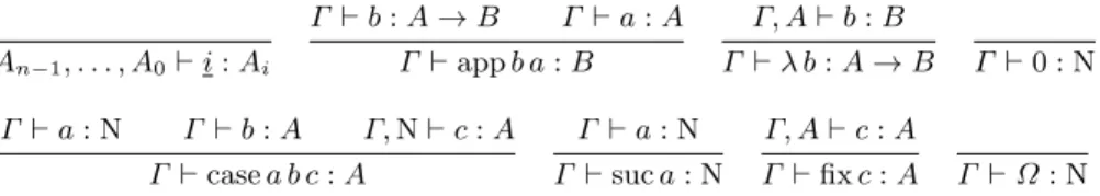
Note that we use de Bruijn indices: the variable n refers to (if it exists) the first λ encountered after crossing n occurrences of λ when going up the syntax tree from the variable to the root. We include the non-terminating program Ω. Terms are assigned types using standard typing rules, displayed in Figure 1.
An−1, . . . , A0` i : Ai Γ ` b : A → B Γ ` a : A Γ ` app b a : B Γ, A ` b : B Γ ` λ b : A → B Γ ` 0 : N Γ ` a : N Γ ` b : A Γ, N ` c : A Γ ` case a b c : A Γ ` a : N Γ ` suc a : N Γ, A ` c : A Γ ` fix c : A Γ ` Ω : N
Fig. 1. Typing rules for PCF
Substitution. A substitution is a sequence of terms, written Γ ` han−1, . . . , a0i : An−1, . . . , A0 if for all 0 ≤ i ≤ n − 1 we have Γ ` ai: Ai. For |Γ | = n we define abbreviations idΓ = hn − 1, . . . , 0i, pΓ,A = hn, . . . , 1i and qΓ,A = 0. We have Γ ` idΓ : Γ and Γ, A ` pΓ,A: Γ . We will often just write id, p, and q.
(case a b c)[γ] = case a[γ] b[γ] c[hγ ◦ p, qi] (suc a)[γ] = suc (a[γ]) 0[γ] = 0 (app f a)[γ] = app (f [γ]) (a[γ]) (fix c)[γ] = fix (c[hγ ◦ p, qi]) Ω[γ] = Ω
(λ f )[γ] = λ (f [hγ ◦ p, qi])
We define the action a[γ] of a substitution ∆ ` γ : Γ on a term Γ ` a : A by induction on a, with i[han−1, . . . , a0i] = ai for variables and following the rules of Figure 2 for term constructors. The composition of substitutions is defined by han−1, . . . , a0i ◦ γ = han−1[γ], . . . , a0[γ]i. When composing substitutions we will sometimes omit the operator ◦ and just use juxtaposition. By abuse of notation, we write hγ, ai for the sequence obtained by adding a at the end of γ.
c →η1 λ (app (c[p]) q)
app (λ a) b →β1 a[hid, bi] a →η2 case a 0 (suc q)
case 0 b c →β2 b case (case a b f ) b 0
f0→γ1 case a (case b b 0
f ) case (suc a) b c →β3 c[hid, ai] (case f (b
0
[p]) fix f →δ f [hid, fix f i] (f0[hpp, qi]))
Ω →Ω Ω app (case a b f ) c →γ2 case a (app b c)(app f (c[p]))
Fig. 3. Reduction rules for PCF
Reduction. We equip PCF with the (context closure of the) reduction rules in Figure 3. The rules are typed : a reduction applies when both sides typecheck. We write ≈ for convertibility, i.e. the contextual equivalence closure of these relations. The two columns of Figure 3 will be treated quite differently in our development. The left hand side contains the computation rules which are used for evaluating a closed term of ground type. The right hand side contains η-expansion and commutating conversions, which are additional rules needed in Section 3.4 for transforming an arbitrary term to its PCF B¨ohm tree.
We will also need head reduction. For that, define head environments as: H[] ::= [] | case H[] b c | app H[] b | λ H[]
Head reduction →h is H[→α] for α ∈ {β1, β2, β3, δ, Ω} a computation rule. Head reduction is deterministic: for each term, at most one head reduction ap-plies. A term a is a head normal form if it is →h-normal. If a →∗ha0 where a0 is →h-normal, then a0 is the head normal form of a.
Non-dependent cwfs. Usually a model of PCF is a cartesian closed category with extra structure. We prefer to use a notion of model which separates contexts and types, and thus more closely matches the structure of our syntax. For that we use categories with families (cwfs) [12]. Cwfs provide a notion of model of dependent type theory which is both close to the syntax, and completely algebraic: it can be presented as a generalized algebraic theory in the sense of Cartmell [7].
Since we do not have dependent types we use non-dependent cwfs, that is cwfs where the set of types Type(Γ ) does not depend on the context Γ . Definition 1. A non-dependent cwf consists of a set of types Type, plus:
– A base category C. Its objects represent contexts and its morphisms represent substitutions. We write ∆ ` γ : Γ for a context morphism from ∆ to Γ . The identity is written Γ ` idΓ : Γ and composition is written γ ◦ δ, or just γδ.
– A functor T : Cop → SetType. For each context Γ and type A this gives a set T (Γ )(A), written Γ ` A, of terms of type A in context Γ . We write Γ ` a : A for a ∈ Γ ` A. For γ : ∆ → Γ a morphism in C, then T (γ)(A) : Γ ` A → ∆ ` A provides a substitution operation, written ∆ ` a[γ] : A. – A terminal object [] of C which represents the empty context and a terminal
morphism hi : ∆ → [] which represents the empty substitution.
– A context comprehension which to an object Γ in C and a type A ∈ Type associates an object Γ ·A of C, a morphism pΓ,A: Γ ·A → Γ of C and a term Γ · A ` qΓ,A : A such that the following universal property holds: for each object ∆ in C, morphism γ : ∆ → Γ , and term a : ∆ ` A, there is a unique morphism θ = hγ, ai : ∆ → Γ ·A, such that pΓ,A◦ θ = γ and qΓ,A[θ] = a. Democratic [8] non-dependent cwfs are equivalent to categories with finite prod-ucts, but mimic more closely the structure of syntax. To describe the intended models of PCF we equip non-dependent cwfs with more structure, as follows. Definition 2. A non-dependent cwf supports PCF, or is a pcf-cwf, iff it is closed under the types and term constructors of Figure 1 (other than variable) and validates the equations and reduction rules of Figures 2 and 3, which have been chosen to make formal sense in an arbitrary non-dependent cwf as well as in the syntax of PCF. (A de Bruijn variable n in PCF is interpreted as an iterated projection q[pn] and all other syntactic constructs have a direct interpretation.)
2.2 Innocent strategies for PCF
We start with a simple operational presentation of the pcf-cwf of innocent well-bracketed strategies playing on (arenas for) PCF types.
N → N → N q OQ q P Q 0 OA q P Q 0 OA 0 P A Fig. 4. A play on N → N → N
Game semantics formalize the intuition that a program is a strategy, and that execu-tion is a play of this strategy against its ex-ecution environment according to rules deter-mined by the type. For instance, a dialogue of type N → N → N could be that of Figure 4. Moves are either Questions (Q) or Answers (A) by either Player (P) or Opponent (O). Ques-tions correspond to variable calls, and Answers to evaluation to terminating calls. The lines between moves are justification pointers: they convey information about thread indexing – here they are redundant, but be-come necessary on higher types. The diagram above should be read as follows: Opponent asks for the output of a function f : N → N → N. This function f (Player) proceeds to interrogate its first argument. This argument is part of the execution environment of f , so it is played by Opponent – if it evaluates to 0, then f evaluates its second argument. If it also evaluates to 0, then f answers 0. A strategy is a collection of such interactions, informing the full behaviour of a program under execution.
The dialogue above, considered as a branch of a strategy, can also be repre-sented syntactically by the term ` λ (λ (case 1 (case 0 0 Ω) Ω)) : N → N → N, where the occurrences of Ω indicate parts of the term for which the dialogue above gives no information. In general a dialogue such as the above where (1) Opponent moves are justified by their immediate predecessor and (2) every An-swer is justified by the last unanAn-swered Question, can always be represented syntactically as a partial term – such dialogues are usually called well-bracketed P-views. In our example, the dialogue is a branch of the strategy for left-plus that first evaluates its first argument (and copies lazily each successor), then the second. The strategy for left-plus contains countably many dialogues. As a typical example, we show the dialogue for the computation of 2 + 2 in Figure 5.
N→N→N q OQ q P Q S OA S P A q OQ q P Q S OA S P A q OQ q P Q 0 OA q P Q S OA S P A q OQ q P Q S OA S P A q OQ q P Q 0 OA 0 P A Fig. 5. left-plus
Representing these plays syntactically and pasting them together, one obtains the infinitary term ` plus : N → N → N defined by
plus = λ (λ (case 1 cc (suc plus1))) cc = case 0 0 (suc cc)
plusn= case 0 (case n 0 (suc cc)) (suc plusn+1)
Here cc stands for copycat, the back-and-forth copy-ing performed by the strategy when evaluatcopy-ing its second argument. Note that the de Bruijn indices grow. Indeed the second argument of case is an abstraction which binds a new variable, so the address of the second argument of f corresponds to larger and larger integers. Alternatively one can say that each Opponent Answer S in the plays provide a possible justifier that has to be crossed before reaching the second argument of f . We call the infinitary term above the PCF B¨ohm tree of left-plus.
The ideas above can easily be extended to represent syntactically (as an infinitary term) any innocent well-bracketed strategy, i.e. set of well-well-bracketed P-views on first-order PCF types N → . . . → N → N. In general how-ever, types of PCF have the form An−1→ . . . → A0→ N, where each Ai has itself the form Ai,pi−1→ . . . → Ai,0→ N. In that case the discussion above still applies to the re-striction of a strategy to its “first-order sub-type”, which provides the backbone of a PCF B¨ohm tree. However, Player also needs to specify its behaviour should Opponent interrogate any of the arguments Ai,j of a Player Question at the root of Ai. For each such Opponent Question, following (co-)inductively the same reasoning, a strategy for Player would inform a new strategy playing on An−1 → . . . → A0 → Ai,j that can be set as an argument to the variable call matching the Player Question under consideration. This presentation of a strategy is called its PCF B¨ohm tree.
PCF B¨ohm trees. We now describe the terms obtained by this process. There are two kinds. On the one hand we define the neutral PCF B¨ohm trees which specify one Player Question (a variable call) along with the Player sub-strategies for the arguments of this call. On the other hand we define PCF B¨ohm trees wrap neutral PCF B¨ohm trees in a case statement, specifying the Player sub-strategies to play if Opponent answers 0 or S. We write Γ `Nee : A if e is a finite neutral B¨ohm tree and Γ `Btt : A if t is a finite PCF B¨ohm trees of type A in context Γ . They are defined as follows:
An−1, . . . , Ai, . . . , A0`Nei : Ai Γ `Nee : A → B Γ `Btt : A Γ `Neapp e t : B Γ, A `Btt : B Γ `Btλ t : A → B Γ `Bta : N Γ `Btsuc a : N Γ `Nee : N Γ `Btt : N Γ, N `Btt0: N Γ `Btcase e t t 0 : N Γ `BtΩ : N Γ `Bt0 : N
Fig. 6. Typing rules for finite PCF B¨ohm trees
These two sets are partially ordered by (the contextual closure of) Ω ≤ a for all a, and their infinitary counterparts are defined as ideals (non-empty down-ward directed sets) for this order [21] – we will often keep this ideal completion implicit. From now on all PCF B¨ohm trees are considered infinitary,
The representation process outlined above yields a PCF B¨ohm tree in this formal sense. Moreover, this PCF B¨ohm tree is an infinitary PCF term, so can be sent back to a strategy using (by continuity) the usual game-theoretic inter-pretation of terms. This operation is inverse to the reification process described above, yielding an isomorphism between PCF B¨ohm trees and innocent strate-gies. In fact the correspondence is so direct that in the remainder of this paper we will identify them, and simply consider PCF B¨ohm trees as our representation of innocent strategies.
This correspondence is nothing new – it is one of the fundamental properties of the game model leading to definability: see eg Theorem 5.1 in [11]. It is easy to adapt this to lazy PCF. It is implicit in McCusker’s definability process for a language with lazy recursive types (see Proposition 5.8 in [18]). We have not spelled out this connection more formally, since it would take too much space to introduce the required game-theoretic machinery.
2.3 Computing operations on strategies by nbe
To conclude this section we present (one aspect of) our result: that we can com-pute operations on innocent well-bracketed strategies, regarded as PCF B¨ohm trees, by nbe. As an example, a Haskell program that, given two infinite PCF B¨ohm trees as input, produces lazily the application of one to the other. All other operations of pcf-cwfs can be defined in an analogous way. In the remaining sec-tions we will then show that application, and all the other pcf-cwf operasec-tions,
satisfy the expected equations, and that we get a pcf-cwf PCFInn of PCF-B¨ohm trees (or innocent, well-bracketed strategies).
The Haskell datatype for representing PCF B¨ohm trees and types of PCF is:
data Tm = ZeroTm | SuccTm Tm | LamTm Tm | CaseTm Tm Tm Tm | VarTm Int | AppTm Tm Tm
data Ty = Nat | Arr Ty Ty
It should be clear to the reader how inhabitants of Tm include representatives for PCF B¨ohm trees, hence for innocent strategies. The first step is to interpret PCF B¨ohm trees in a semantic domain D, which is a hoas version of Tm:
data D = ZeroD | SuccD D | LamD (D -> D) | CaseD D D (D -> D) | VarD Int | AppD D D
We then introduce two semantic operations appD :: D -> D -> D for ap-plication, and caseD :: D -> D -> (D -> D) -> D for case construction.
appD (LamD f) d’ = f d’
appD (CaseD e d f) d’ = CaseD e (appD d d’) (\x -> appD (f x) d’) appD (VarD n) d’ = AppD (VarD n) d’
appD (AppD e d) d’ = AppD (AppD e d) d’ caseD ZeroD e’ f’ = e’
caseD (SuccD d) e’ f’ = f’ d
caseD (CaseD e d f) e’ f’ = CaseD e (caseD d e’ f’) (\x -> caseD (f x) e’ f’) caseD (AppD e d) e’ f’ = CaseD (AppD e d) e’ f’ caseD (VarD i) e’ f’ = CaseD (VarD i) e’ f’
We can interpret a PCF B¨ohm tree in the semantic domain D by the function eval :: Tm -> [D] -> D. It takes a term and interprets it in a given environ-ment, encoded as a list of elements of the domain.
eval ZeroTm env = ZeroD
eval (SuccTm t) env = SuccD (eval t env)
eval (LamTm t) env = LamD (\x -> eval t (x:env)) eval (CaseTm t1 t2 t3) env = caseD (eval t1 env) (eval t2 env)
(\x -> eval t3 (x:env)) eval (VarTm i) env = env !! i
eval (AppTm t1 t2) env = appD (eval t1 env) (eval t2 env)
An element of the semantic domain can be read back to a term using the function readbackD :: Int -> D -> Tm, defined as follows.
readbackD n ZeroD = ZeroTm
readbackD n (SuccD d) = SuccTm (readbackD n d)
readbackD n (LamD f) = LamTm (readbackD (n+1) (f (VarD n))) readbackD n (CaseD e d f) = CaseTm (readbackD n e) (readbackD n d)
(readbackD (n+1) (f (VarD n))) readbackD n (VarD i) = VarTm (n-i-1)
Finally, we obtain readback :: Int -> ([D] -> D) -> Tm as
readback n f = readbackD n (f [VarD (n-i-1) | i <- [0..(n-1)]])
The application of a PCF B¨ohm tree (innocent strategy) Γ `Bt t : A → B to Γ `Btt0 : A with |Γ | = n can now be computed lazily as app n t t’, where app :: Int -> Tm -> Tm -> Tm is defined by
app n t t’ = readback n (\x -> appD (eval t x) (eval t’ x))
We will in the following sections prove that this simple definition computes the claimed result. We can define functions for all other pcf-cwf combinators in a similar way, and prove that they satisfy the pcf-cwf-laws. In this way we get a pcf-cwf PCFInn which is an alternative nbe-based presentation of the innocent strategies model of PCF – these will come as a by-product of a nbe procedure producing the innocent strategy for a term.
3
The domain interpretation
To prove the correctness of the nbe program we use its denotational semantics in Scott domains. We first show that the interpretation function is sound w.r.t. syntactic conversion and computationally adequate. Then we show that the η-expanded interpretation of a term is equal to that of its PCF B¨ohm tree.
3.1 A semantic domain
D and its combinators. The Haskell datatype D can be interpreted as a Scott domain D which is the solution of the domain equation given by the constructors:
LamD: (D → D) → D SucD: D → D 0D: D AppD: D → D → D CaseD: D → D → (D → D) → D VarD: N → D We write ΩD for the bottom element. The two semantic operations appD: D → D → D and caseD : D → D → (D → D) → D are defined as their Haskell counterparts in Section 2.3.
Interpretation of PCF. Let Tm be the set of elements of the raw syntax of PCF. If E is a set, [E] denotes the set of lists of elements of E. As for substitutions, we write hi for the empty list. If ρ ∈ [D] and d ∈ D, we write ρ :: d for the addition of d at the end of ρ3Finally, ρ(i) is the i-th element of ρ starting from the right and from 0, if it exists, and ΩDotherwise.
The interpretation of PCF is defined as a functionJ−K : Tm → [D] → D: [[fix f ]] ρ =F
n∈N(λd. [[f ]] (ρ :: d)) n(Ω
D) [[n]] ρ = ρ(n) [[app s t]] ρ = appD([[s]] ρ) ([[t]] ρ) [[suc a]] ρ = SucD([[a]] ρ)
[[λ t]] ρ = LamD(λx.[[t]] (ρ :: x)) [[Ω]] ρ = ΩD [[case a b c]] ρ = caseD([[a]] ρ) ([[b]] ρ) (λx. [[c]] (ρ :: x)) [[0]] ρ = 0D
3
This notational difference from the Haskell program ensures that the order of envi-ronments matches that of the context.
It is extended to substitutions γ = han−1, . . . , a0i by [[γ]] ρ = h[[an−1]] ρ, . . . , [[a0]] ρi.
3.2 Soundness for conversion
Here, we prove that the interpretation described above is sound with respect to conversion in PCF. Reduction rules of PCF come in three kinds: the computation rules (β1, β2, β3, δ, Ω), the commutation rules (γ1, γ2) and the η-expansion rules (η1, η2). Soundness w.r.t. computation rules follows from standard (and simple) verifications, and we verify only the commutation and η-expansion rules. Commutation rules. The interpretation of PCF validates γ1 and γ2. Lemma 1. For all d1, d2, d3∈ D and f, f1, f2∈ D → D, we have:
appD(caseDd1d2f ) d3= caseDd1(appDd2d3) (λx. appD(f x) d3) caseD(caseDd1d2f1) d3f2= caseDd1(caseDd2d3f2) (λx. caseD(f1x) d3f2) Proof. We apply Pitts’ co-induction principle [19] for proving inequalities in re-cursively defined domains. The proof proceeds by defining a relation R containing the identity relation on D and all pairs (for d1, d2, d3∈ D and f ∈ D → D):
(appD(caseDd1d2f ) d3, caseDd1(appDd2d3) (λx. appD(f x) d3)) Then, R is a bisimulation. For d1 = ΩD, VarDi, AppDd01d02, LamDf0, 0D or SucDd0, both sides evaluate to the same, so the bisimulation property is trivial. For d1 = CaseDd01d02f0, by direct calculations both sides start with CaseD, followed by arguments related by R. By Pitts’ result [19] the equality follows. η-expansion rules. Note that these cannot be true in general since the interpre-tation ignores type information. So we define a semantic version of η-expansion:
ηNd = caseDd 0D(λx. ηNx) ηA→Bd = LamD(λx. ηBappDd (ηAx)) It extends to environments by η[]ρ = [], ηΓ,A[] = (ηΓ[]) :: ΩDand ηΓ,A(ρ :: d) = (ηΓρ) :: (ηAd). For f : [D] → D we define ηΓ `Af = λρ. ηA(f (ηΓ ρ)).
From semantic expansion we get a typed notion of equality up to η-expansion in the domain: for a type A and elements d, d0 ∈ D we write d =Ad0 iff ηAd = ηAd0. This generalizes to f =Γ `Af0in the obvious way. We now prove that syntactic η-expansion is validated up to semantic η-expansion.
It is easy to see that for Γ ` b : A → B we haveJbK =Γ `A→BJλ (app b[p] 0)K and also to verify the η-rule for N. However, reduction rules are closed under context, so we need to check that typed equality is a congruence.
This relies on the fact that the interpretation of terms cannot distinguish an input from its η-expansion. To prove that we start by defining a realizability predicate on D, by d N for all d ∈ D, and d A → B iff for all d0 A, (1) appDd d0 =B appDd (ηAd0) and (2) appDd d0 B. This predicate generalizes
to contexts (written ρ Γ ) in the obvious way. We observe by induction on A that η-expanded elements of D are realizers: for all d ∈ D, ηAd A. But the interpretation of terms, despite not being η-expanded, also satisfy it. Indeed we prove, by induction on typing judgments, the following adequacy lemma. Lemma 2. For Γ ` a : A, ρ Γ , then (1)JaK ρ =AJaK (ηΓ ρ) and (2)JaK ρ A. It is then immediate that the interpretation of term constructors preserves typed equality. All conversion rules hold up to typed equality in D, which is a congru-ence w.r.t. the interpretation of terms. Putting it all together we conclude: Proposition 1 (Soundness). For Γ ` a, a0: A with a ≈ a0,
JaK =Γ `AJa 0
K. 3.3 Computational adequacy
As a step towards our main result, we prove computational adequacy:
Proposition 2. If Γ ` a : A andJaK 6=Γ `A ΩD then a has a head normal form. First, we reduce the problem to closed terms by noting two properties: – Firstly, Γ, A ` b : B has a head normal form iff λ b has,
– Secondly, JbK =Γ,A`B ΩD iff Jλ bK =Γ `A→B ΩD, as can be checked by a simple calculation.
So we abstract all free variables of a term and reason only on closed terms. We now aim to prove it for closed terms. The proof has two steps: (1) we prove it for closed terms of ground type using logical relations, and (2) we deduce it for closed terms of higher-order types. To obtain (2) from (1) we will need to temporarily enrich the syntax with an error constant ∗. This ∗ has all types – we write Γ `∗ a : A for typing judgments in the extended syntax. We also add two head reductions app ∗ a →h∗ and case ∗ a b c →h∗.
We also need to give an interpretation of ∗ in D. At this point it is tempting to enrich the domain D with a constructor for ∗. Fortunately we can avoid that; indeed the reader can check that setting J∗K ρ = CaseDΩDΩD(λx. ΩD) = ∗D, the interpretation validates the two reduction rules above. Note that the term ∗ is only an auxiliary device used in this section: we will never attempt to apply nbe on a term with error, so this coincidence will be harmless.
Ground type. We first define our logical relations. Definition 3. We define a relation ∼n
N between closed terms `∗ a : N and elements of D by induction on n. First a ∼0
Nd always. Then, a ∼ n+1
N d iff either d = ΩD, or a →∗h0 and d = 0D, or a →∗h∗ and d = ∗D, or finally, if a →∗
hsuc a0 and d = SucDd0 and a0∼n
Nd0. We then define a ∼N d iff for all n ∈ N, a ∼ n N d. Finally, b ∼A→B d iff for any a ∼Ae, app b a ∼BappDd e.
This relation is closed under backward head reduction, and satisfies the con-tinuity property that for any ω-chain (di)i∈N, if a ∼Adifor all i then a ∼Atidi. The fundamental lemma of logical relations follows by induction on a.
Lemma 3. For any term Γ `∗a : A, for any δ ∼Γ ρ, we have a[δ] ∼AJaK ρ. By definition of ∼A, computational adequacy follows for closed terms of type N.
Higher-order types. Suppose ` a : An−1→ . . . → A0 → N = A satisfiesJaK 6=A ΩD. We need to show that a has a head normal form, but our previous analysis only applies to terms of ground type. By hypothesis we know that forJaK there are some arguments dn−1, . . . , d0 makingJaK non-bottom. However, in order to apply our earlier result for ground type, we need to find syntactic counterparts to dn−1, . . . , d0 – and there is no reason why those would exist. So instead we replace the dis with ∗D, which does have a syntactic counterpart.
The core argument is that replacing arguments ofJaK with ∗Donly increases chances of convergence. To show that we introduce:
Definition 4. We define .n
N⊆ D2 by induction on n. Let d1.0Nd2⇔ > and
d1.n+1N d2⇔
If d1= d2= 0D
If d1= SucDd01, d2= SucDd20 and d01.nNd02 If d1= ΩD or d2≥ ∗D
We set d1.Nd2 iff for all n ∈ N, d1.nNd2. We lift this to all types by stating that d1.A→Bd2 iff for all d01.Ad02, appDd1d01.BappDd2d02.
This generalizes to a relation on environments ρ1 .Γ ρ2, but unlike what the notation suggests, .A is not an ordering: it is neither reflexive, nor transitive, nor antisymmetric. However, for all A and d ∈ D we have ΩD.Ad .A∗D.
The following fundamental lemma is proved by induction on a. Lemma 4. For any term Γ `∗a : A, for any ρ1.Γ ρ2,JaK ρ1.AJaK ρ2.
Putting the ingredients above together, we prove the following lemma. Lemma 5. For `∗a : A, d .AJaK and d 6=AΩD, a has a head normal form. Proof. For N, assume there is d .NJaK such that d 6=NΩD, so d 6= ΩD. It follows by definition of .N that eitherJaK = ∗D, or d and JaK respectively start both with 0Dor both with SucD. But by Lemma 3 we have a ∼NJaK, so by definition of logical relations, a has a head normal form.
For A → B, take `∗ b : A → B and assume there is d .A→B JbK such that d 6=A→B ΩD. So there is d0 ∈ D such that appDd (ηAd0) 6=B ΩD. But we have observed above that ηAd0.A∗D. Therefore, by definition of .A→B, we have:
appDd (ηAd0) .BappDJbK ∗D=Japp b ∗K
By induction hypothesis, app b ∗ has a head normal form. But head reduction is deterministic, and any potentially infinite head reduction chain on b would transport to app b ∗, so b has a head normal form.
Finally, it remains to deduce computational adequacy for closed terms. But for arbitrary `∗ a : A such thatJaK 6=A ΩD, by Lemma 4 we haveJaK .A JaK, so we are in the range of Lemma 5 – therefore, a has a head normal form.
3.4 PCF B¨ohm trees defined by repeated head reduction
In the next section we show how the PCF B¨ohm tree of a term can be computed by nbe. We also show that the result of this computation coincides with the traditional way of defining a PCF B¨ohm tree as obtained by repeated head reduction. This definition relies on the following lemma.
Lemma 6. The system {→γ1, →γ2} of commutations is strongly normalizing.
Proof. Local confluence follows from a direct analysis of the (two) critical pairs, and one gets a decreasing measure by defining |a| = 1 on all leaves of the syntax tree, |case a b f | = 2|a| + max(|b|, |f |) and |app a b| = 2|a| + |b| and | − | behaves additively on all other constructors.
The PCF B¨ohm tree of a term. The PCF B¨ohm tree BT(a) of a term Γ ` a : A is defined as follows. If A = N and a has no head normal form then BT(a) = Ω. Otherwise we convert a to head normal form and then to →γ1,γ2-normal form
a0 by Lemma 6 which is still a head normal form. The only possible cases are: – BT(a) = 0 if a0 = 0.
– BT(a) = suc BT(a00) if a0= suc a00
– BT(a) = case (app i−−−−→BT(aj)) 0 (suc BT(0)) if a0= app i −→aj – BT(a) = case (app i−−−−→BT(aj)) BT(b) BT(c) if a0= case (app i −→aj) b c.
If A = B → C then BT(a) = λ BT(app (a[p]) 0). (BT(a) could be more explicitly defined as an ideal of finite approximations, see e.g. [14] for details.)
Together with the earlier results, we get the main result of this section. Proposition 3. If Γ ` a : A then Γ `BtBT(a) : A and ηΓ `AJaK = JBT(a)K. Proof. As we aim to prove the equality of two elements of D we use again Pitts’ method [19] and define the following relation
R = {(JBT(a)K (ηΓρ), ηA(JaK (ηΓρ))) | Γ ` a : A & ρ ∈ [D]}
and show that it is a bisimulation. Proposition 1 ensures that the conversion steps needed to transform a term to its PCF B¨ohm tree are sound in the model, Proposition 2 ensures that both sides are ΩDat the same time.
This ends the core of the technical development. The same proof scheme can be used to show that the game interpretation of Section 2.2 validates conversion to PCF B¨ohm trees. Details can be obtained by adapting McCusker’s proof [18].
4
Game semantics of PCF based on nbe
Normalization by evaluation. We are now ready to show the correctness of an nbe algorithm which computes innocent strategies for infinitary terms. Recall that in Section 2.2 we defined PCF B¨ohm trees as ideals of finite PCF B¨ohm
trees. The same construction on arbitrary PCF terms yields a notion of infinitary term on which BT andJ−K automatically extends, along with Proposition 3.
The readback function Rn : ([D] → D) → Tm is the semantic counterpart of the Haskell readback function in Section 2.3. The following is proved on finitary terms by a direct induction and extends to PCF B¨ohm trees by continuity. Lemma 7. If Γ `Btt : A is a PCF B¨ohm tree with |Γ | = n, then RnJtK = t.
We now define an nbe algorithm which maps a PCF term to its PCF B¨ohm tree, and use this lemma together with Proposition 3 to show its correctness: Theorem 1. Let Γ ` a : A be an (infinitary) PCF term. If nbe(a) = Rn(ηΓ `AJaK), where |Γ | = n, then nbe(a) = BT(a).
The pcf-cwf of PCF B¨ohm trees. We conclude this paper by showing how to recover the Hyland-Ong game model of PCF, up to isomorphism of pcf-cwfs. If d ∈ D, say that d has (semantic) type A iff ηAd = d. Likewise a function f : [D] → D has type Γ ` A iff ηΓ `Af = f , and a function γ : [D] → [D] has type Γ ` ∆ iff it is obtained by tupling functions of the appropriate types. This generalizes to a pcf-cwf D having PCF contexts as objects and functions (resp. elements) of the appropriate type as morphisms (resp. terms).
As a pcf-cwf, D supports the interpretation of PCF. But the plain domain interpretationJaK (of Section 3) of a PCF B¨ohm tree Γ `Bta : A automatically has semantic type Γ ` A, and so is a term in the sense of D. Furthermore, this map from PCF B¨ohm trees to D is injective by Theorem 1. Finally, the image of PCF B¨ohm trees in D is closed under all pcf-cwf operations: each of these can be replicated in the infinitary PCF syntax then normalized using nbe, yielding by Theorem 1 and Proposition 3 a PCF B¨ohm tree whose interpretation matches the result of the corresponding operation in D. So, the interpretation of PCF B¨ohm trees forms a sub-pcf-cwf of D, called PCFInn, satisfying:
Theorem 2. PCFInn is isomorphic to the pcf-cwf of PCF contexts/types, and innocent well-bracketed strategies between the corresponding arenas.
If we unfold this definition we get the Haskell program for application in Sec-tion 2.3 and similar programs for composiSec-tion and the other pcf-cwf operaSec-tions. The pcf-cwf laws for these programs, such as associativity of composition, β, and η, follow from the corresponding laws for their domain interpretation in D.
Acknowledgments. The first author acknowledges the support of French ANR Project RAPIDO, ANR-14-CE25-0007.
References
1. Andreas Abel. Normalization by Evaluation: Dependent Types and Impredicativ-ity. Institut f¨ur Informatik, Ludwig-Maximilians-Universit¨at M¨unchen, May 2013. Habilitation thesis.
2. Andreas Abel, Klaus Aehlig, and Peter Dybjer. Normalization by evaluation for Martin-L¨of type theory with one universe. In ”23rd Conference on the Mathe-matical Foundations of Programming Semantics, MFPS XXIII, Electronic Notes in Theoretical Computer Science, pages 17–40. Elsevier, 2007.
3. Samson Abramsky, Radha Jagadeesan, and Pasquale Malacaria. Full abstraction for PCF. Inf. Comput., 163(2):409–470, 2000.
4. Klaus Aehlig and Felix Joachimski. Operational aspects of untyped normalisation by evaluation. Mathematical Structures in Computer Science, 14(4), 2004. 5. Roberto Amadio and Pierre-Louis Curien. Domains and lambda-calculi.
Num-ber 46. Cambridge University Press, 1998.
6. Ulrich Berger and Helmut Schwichtenberg. An inverse to the evaluation functional for typed λ-calculus. In Proceedings of the 6th Annual IEEE Symposium on Logic in Computer Science, Amsterdam, pages 203–211, July 1991.
7. John Cartmell. Generalized algebraic theories and contextual categories. Annals of Pure and Applied Logic, 32:209–243, 1986.
8. Pierre Clairambault and Peter Dybjer. The biequivalence of locally cartesian closed categories and Martin-L¨of type theories. Mathematical Structures in Computer Science, 24(5), 2013.
9. Pierre Clairambault and Andrzej S. Murawski. B¨ohm trees as higher-order recur-sive schemes. In IARCS Annual Conference on Foundations of Software Technology and Theoretical Computer Science, FSTTCS 2013, December 12-14, 2013, Guwa-hati, India, pages 91–102, 2013.
10. Pierre-Louis Curien. Abstract B¨ohm trees. Mathematical Structures in Computer Science, 8(6):559–591, 1998.
11. Pierre-Louis Curien. Notes on game semantics. From the author’s web page, 2006. 12. Peter Dybjer. Internal type theory. In Stefano Berardi and Mario Coppo, edi-tors, Types for Proofs and Programs, International Workshop TYPES’95, Torino, Italy, June 5-8, 1995, Selected Papers, volume 1158 of Lecture Notes in Computer Science, pages 120–134. Springer, 1995.
13. Peter Dybjer. Program testing and the meaning explanations of intuitionistic type theory. In Epistemology versus Ontology - Essays on the Philosophy and Foundations of Mathematics in Honour of Per Martin-L¨of, pages 215–241. 2012. 14. Peter Dybjer and Denis Kuperberg. Formal neighbourhoods, combinatory
B¨ohm trees, and untyped normalization by evaluation. Ann. Pure Appl. Logic, 163(2):122–131, 2012.
15. Andrzej Filinski and Henning Korsholm Rohde. Denotational aspects of untyped normalization by evaluation. Theor. Inf. and App., 39(3):423–453, 2005.
16. Russell Harmer, Martin Hyland, and Paul-Andr´e Melli`es. Categorical combinators for innocent strategies. In 22nd IEEE Symposium on Logic in Computer Science, Wroclaw, Poland, Proceedings, pages 379–388. IEEE Computer Society, 2007. 17. J. M. E. Hyland and C.-H. Luke Ong. On full abstraction for PCF: I, II, and III.
Inf. Comput., 163(2):285–408, 2000.
18. Guy McCusker. Games and full abstraction for FPC. Inf. Comput., 160(1-2):1–61, 2000.
19. Andrew M. Pitts. A co-induction principle for recursively defined domains. Theor. Comput. Sci., 124(2):195–219, 1994.
20. Gordon D. Plotkin. LCF considered as a programming language. Theor. Comput. Sci., 5(3):223–255, 1977.
21. Gordon D. Plotkin. Post-graduate lecture notes in advanced domain theory (in-corporating the ”Pisa Notes”). Dept. of Computer Science, Univ. of Edinburgh, 1981.