Publisher’s version / Version de l'éditeur:
Water Resources Research, 7, 2, pp. 323-333, 1971-04
READ THESE TERMS AND CONDITIONS CAREFULLY BEFORE USING THIS WEBSITE. https://nrc-publications.canada.ca/eng/copyright
Vous avez des questions? Nous pouvons vous aider. Pour communiquer directement avec un auteur, consultez la première page de la revue dans laquelle son article a été publié afin de trouver ses coordonnées. Si vous n’arrivez pas à les repérer, communiquez avec nous à [email protected].
Questions? Contact the NRC Publications Archive team at
[email protected]. If you wish to email the authors directly, please see the first page of the publication for their contact information.
NRC Publications Archive
Archives des publications du CNRC
This publication could be one of several versions: author’s original, accepted manuscript or the publisher’s version. / La version de cette publication peut être l’une des suivantes : la version prépublication de l’auteur, la version acceptée du manuscrit ou la version de l’éditeur.
Access and use of this website and the material on it are subject to the Terms and Conditions set forth at
Predicting the date of lake ice breakup
Williams, G. P.
https://publications-cnrc.canada.ca/fra/droits
L’accès à ce site Web et l’utilisation de son contenu sont assujettis aux conditions présentées dans le site LISEZ CES CONDITIONS ATTENTIVEMENT AVANT D’UTILISER CE SITE WEB.
NRC Publications Record / Notice d'Archives des publications de CNRC:
https://nrc-publications.canada.ca/eng/view/object/?id=c78936b8-b9a4-45d5-9bb7-550838820706 https://publications-cnrc.canada.ca/fra/voir/objet/?id=c78936b8-b9a4-45d5-9bb7-550838820706WATER RESOURCES RESEARCH A P R I L 1971
?;
Af?2%3>
Predicting the Date
of
Lake Ice Breakup
G. P . WILLIAMS
Division of Building Research, National Research Council, Ottawa, Ontario, Canada
Abstract. Standard deviations for lake breakup dates were calculated for all lakes in Canada with reasonably long breakup records and for five lakes in Wisconsin with long-term records. Standard deviations were about 13 days for coastal lakes and 7-11 days for continental lakes. The accuracy of the melting degree day method of predicting breakup dates were in- vestigated for 12 of these lakes; standard deviations ranged from 3.3-8.0 days. Regression equations for predicting breakup dates were developed from past breakup and air temperature records for the 12 lakes; standard errors ranged from 1.6-4.3 days. General forecast guidelines were developed for application to lakes with limited breakup records. The equations and fore- cast guidelines are suitable only for continental lakes where wind and river inflow effects are not dominant.
INTRODUCTION tionnaires t o observers a t numerous lakes across
The date of lake ice breakup, defined as the day on which a lake is completely cleared of ice, marks the beginning of the navigation season for northern lakes used for transportation. For several weeks prior to breakup, ice covers on these lakes a r e in a weakened condition and cannot be used b y either ski equipped or float planes. A prediction of the duration of the pe- riod when supplies cannot be flown in would be of value in the planning of construction, logging, and mineral and oil exploration activities. If t h e date of breakup could be predicted, it would be easier t o schedule supplies and logging drives, and full advantage could be taken of a short open water season. T o date, there is only lim- ited published information available on the prob-
lem
[Williams,
19651.This paper presents the results of a n investi- gation of the accuracy with which the actual date of breakup can be predicted by using past breakup and air temperature records and cur- rent weather information from meteorologic stations. Weather records for this analysis were obtained from the records of the Canadian ineteorologic stations published monthly b y the Canadian Meteorological Branch of the Depart- ment of Transport and from Allen [1964]. In- formation on the effect of wind on breakup was obtained through the courtesy of t h e Canadian Meteorological Branch, which distributed ques-
Canada.
VARIABILITY O F BREAKUP DATES O F LAKES
The standard deviation of breakup dates, cal- culated from past breakup records, is a meas- ure of the variability of the date of lake ice breakup. Since breakup dates a r e distributed r~ormally [Williams, 19681, the standard devia- tion can be used t o calculate the probability t h a t breakup will occur within a n y particular period. For-example, if the standard deviation of breakup dates for a given lake is 8 days, breakup will occur within zk8 days of the average breakup date about 68% of the time a n d within & I 6 days about 95% of the time.
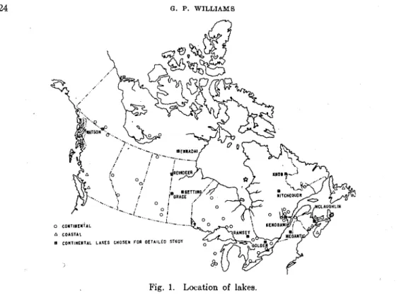
The estimated standard deviation of breakup date was calculated for all lakes in Canada with a reasonably long breakup record. The estimated standard deviation was also calculated from long-term records of five lakes i n Wis- consin [Ragotzkie, 19601. Figure 1 gives their location. Estimated standard deviations, some- times referred t o as estimated standard devia-
,
tions of t h e universe [Ezekiel, 19531 because of adjustment for the number of observations, will be referred t o as standard deviations. Table 1 shows the average standard deviation for lakes subdivided according to length of record. Lakes subject t o mild, coastal weather and consequently having thin ice covers are listed as 'coastal' lakes t o distinguish them fromin-
G . P . WILLIAMS
n
Fig. 1. Location of lakes.
land 'continental' lakes subject to more extreme weather conditions.
The standard deviation for coastal lakes was about 13 days; for continental lakes, 7-11 days. These results compare reasonably well with similar calculations for Swedish lakes with long- term records [Eriksson, 19201. I n the north of Sweden, the standard deviation is 10 days; in mid-Sweden, 15 days; and in the southern coastal regions, 20 days. The period between earliest and latest breakup dates (95% of the time) is 3 0 4 0 days for continental lakes and 50 days or more for coastal lakes.
The wide fluctuation in yearly breakup dates is primarily due to variations in weather dur- ing the ice melting period. A cold, late spring results in delayed breakup; a warm, early spring results in early breakup. Although the process of melting is complex [Williams, 19671, air temperature is one of the most important variables affecting the degeneration of lake ice. The importance of air temperature may be illustrated by comparing air temperature and breakup records for years when abnormal con- ditions prevailed. I n 1945, for example, breakup averaged 15-25 days earlier than normal, and March air temperatures were 10°F-16°F above
normal over an extensive area of eastern Can- ada (Figure 2). I n 1947, over generally the same region, breakup averaged 12-16 days late, and April air temperatures were from 6°F-10°F below normal. On occasion, abnor- mal air temperatures can affect the breakup date of lakes over even more extensive areas. A late breakup was observed in 1956 at almost all lakes across Canada where records were kept.
TABLE 1. Estimated Standard Deviation for Breakup Date for Some Lakes in North America Number Length of Breakup Average Standard of Lakes Record, years Deviation, days
Continental Lakes 28 5-10 7.1 8 11-20 7.9 8 2140 8.2 3* 4&70 8.7 2* 10&105 10.9 Coastal Lakes 6 5-10 12.7 4 19-23 13.0
*
Obtained from records of lakes in Wisconsin [Ragotzkie, 19601.Ice BI Below normal air temperatures during the spring offset the many local factors, such as depth, size and shape of lake, ice thickness, and wind, that can influence the date ice clears from a lake.
ANALYSIS O F SELECTED LAKES
I n the initial stages of the study, an attempt was made to develop techniques for predicting breakup dates. These techniques were based on several parameters that can affect lake ice breakup, such as solar radiation, wind velocity, and ice thickness. Unfortunately, adequate rec- ords of these parameters were not available a t meterologic stations near lakes where breakup dates had been recorded. Subsequent analysis was therefore based only on air temperature data, which are usually available from past rec- ords and are part of routine meteorologic fore- casts.
Twelve continental lakes were chosen for de- tailed analysis in investigating the accuracy with which breakup dates can be predicted from
MARCH AIR TEMPERATURE
1945 + I 0 - t16 O F
HUDSON.S
\
D
ABOVE NORMALFig. 2. Dependence of breakup date on air
temperature.
available breakup and air temperature records. Several factors determined the choice of lakes, the most important being availability of me- teorologic records of solar radiation or hours of sunshine, air temperature, and wind. speed. Although the solar radiation records proved unsatisfactory because of missing or incomplete records, the lakes were originally chosen on the assum~tion that radiation records could be used in the analysis. Lakes were excluded where wind or river runoff would be major factors affecting breakup. Although wind is a factor in clearing ice from some of the lakes chosen, it was assumed that air temperature rather than wind was dominant. Lakes with 20 years or more of record .were excluded because either basic meteorologic data were missing or the size of the lake indicated that wind would be the dominant factor determining breakup.
If the lakes with the longest breakup record could have been used in the analysis, allowance would have had to be made in the statistical analysis for changes in breakup date caused by climatic fluctuation. Long term breakup records available in North America show that from about 1870-1940 breakup of lakes oc- curred a t progressively earlier dates [Williams, 19701. A significant increase in spring air tem- perature occurred during the same period [Thomas, 19681. Since about 1940, there has been no apparent trend for breakup to be- come earlier or later. The gradual change in breakup dates may explain the tendency for the standard deviation to increase with length of record (Table 1 ) .
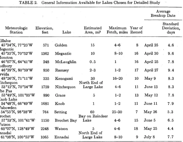
The lakes and the names and locations of meteorologic stations from which air tempera- ture records were obtained are listed in Table 2. Estimated area, estimated maximum fetch, average date of breakup, and standard devia- tion are also tabulated. Available breakur, rec- ords were too limited to warrant arranging the data according to lakes with comparable depth, area, shape, or orientation. The observation sites include long, narrow lakes, such as Setting; small lakes, such as Knob or McLaughlin; and parts of larger lakes, such as Brochet Bay on Reindeer Lake.
Two methods of predicting breakup dates were investigated. The melting degree day method attempts to estimate the date of breakup from the number of melting degree days that
326 G. P. WILLIAMS
TABLE 2. General Information Available for Lakes Chosen for Detailed Study Average Breakup Date
Standard Meteorologic Elevation, Estimated Maximum Year of Deviation,
Station feet Lake Area, mi2 Fetch, miles Record days Killaloe 45 '34'N, 77 "25'W Megantic 45 "35'N, 70°52'W Moncton 46"07'N, M041'W Sudbury 46"29'N, 80°59'W Arvida 48"26'N, 71 "11'W Nitchequon 53 "12'N, 70 "54'W The Pas 53 049'N1 101 "05'W Knob Lake 54 04S1N, 66 "49'W Wabowden 54'55'N, 98'38'W Brochet 57"53'N, 101 "41'W Watson 60°07'N, 128'49'W Ennadai Golden 15 Megantic 10 Ramsey 2-3 Kenoganii 30 North End of Nitchequon Large Lake
Grace a
Knob 1
Setting 60 Bay on Reindeer Brochet Bay Lake
Watson 5 North End of April 25 April 30 April 25 April 27 May 9 June 13 May 12 June 11 May 26 June 5 May 25
61 "08'N, 100°55'W 1065 Ennadai Lsrge Lske 8-10 9 July 8 7.7 Elevation is given in feet above sea level.
accumulate before breakup occurs [Stankiewicz,
19471. T h e .regression equation method cor-
relates t h e duration of t h e ice melt period with t h e date of the s t a r t of significant melting and deviations from average air temperature during the melt period. T h e melt period is defined a s t h e period from t h e date on which significant melting starts t o t h e date when ice clears t h e lake. T h e s t a r t of significant melting was de- fined a s t h e date when accumulated degree days reached 50.
time t h e daily mean air temperature first rises above 32°F until t h e date of breakup for each year for each of t h e 12 lakes. T h e average number of degree days required t o clear ice TABLE 3. Standard Deviation and Accumulated
Melting Degree Days to Breakup Date Average
Accumulated Standard Standard Melting, Deviation, Deviation, Lake degree days degree days days Regression equations were developed for each
Golden 210 46 6.6
of t h e 12 lakes by multiple correlation analysis Megantic 236 67 8 . 0 of available breakup and air temperature rec- McLaughlin 203 41 5.5 ords. T h e equations were further analyzed for Ramsey 194 54 5.7 presentation in a general form t h a t could be Kenogami 3.52 32 3 . 3 Nitchequon 347 46 4.1 of value for forecasting breakup for lakes with
Grace 269 67 5.7
limited breakup records. Knob 249 59 6 . 3
Setting 367 52 4.7
MELTING DEGREE] DAY M ~ H O D Brochet Bay 334 65 6 . 4 Melting degree days were accumulated by
z,":gi
372 56 4.7 537 76 4 . 8 using a base temperature of 32°F from t h eIce Breakup 327 from the lakes and the standard deviations are
shown in Table 3.
Standard deviations in melting degree days
TABLE 4. Duration of Melt Periods, Standard Deviations, and Average Dates of Start of
Significant Melt were converted to days by dividing by average
values of melting degrees for a single day during the melt period. For example, the aver- age daily air temperature during the melt period a t Ennadai Lake is 48°F. Therefore, on the average, there are 16 melting degree days dur- ing a single day. The standard deviation is thus calculated to be 76/16, or 4.8 days. This con- version is not completely satisfactory, because melting degree days late in the melt period can differ from the average. It was necessary, however, in order to compare the results ob- tained by the melting degree day method with those of other methods of forecasting.
The standard deviation for the melting degree day method for the 12 lakes ranged from 3.3- 8.0 days. For some lakes, such as Kenogami or Nitchequon, these deviations are considerably less than standard deviations of breakup dates. For other lakes, such as Megantic and Golden, standard deviations are about equal to or greater than those calculated from the distribution of breakup dates.
The melting degree day method is particularly unsuitable for forecasting the breakup of large lakes. Accumulated melting degree days and standard deviations were calculated for Cold Lake with an estimated area of 140 square miles and Big Trout Lake with an area of 340 square miles. Accumulated melting degree days were 512 and 537, respectively, with standard deviations of about 12 days. Air temperatures measured a t shore stations of large lakes are probably higher than air temperatures over the extensive expanses of melting ice, and the re- sulting values for accumulated melting degree days are relatively high. The variable influence of wind and currents in clearing ice from these large lakes probably contributes to the rela- tively large standard deviations. Similar results would probably be obtained for the main body of Reindeer Lake, where according to the local observer, breakup occurs about 2 weeks later than it does a t Brochet Bay.
One shortcoming of the melting degree day method is t h a t degree days accumulated in the early stages of melt are given the same weight as degree days accumulated during advance stages of melt. I n the later stages, not only is
Average
Average Dnte Duration of Standard of Start of Melt Period, Deviation, Lake Melt Period days to clear days Golden March 31 Megantic April 8 McLaughlin April 3 Ramsey April 8 Kenogami April 7 Nitcheyon May 16 Grace April 22 Knob May 17 Setting April 25 Brochet Bay May 8 Watson April 26 Ennadai June 8
the available solar radiation usually greater, but the percentage of incoming radiation absorbed because of reduced surface albedo is greater as v d l . Several attempts were made to improve
!he melting degree day method by using base
' 2mperatures higher than 32°F and by putting more weight on degree days accumulated late in the melt season. These attempts, although un- successful, provided the basis for the regression equation method of forecasting breakup dates.
REGRESSION EQUATION METHOD
The first step in the regression equation analy- sis was to calculate for each year and each lake the date on which significant melting was as- sumed -to start. A study of past records indi- cated that after 50 degree days, daily minimum air temperatures tended to remain above 32°F. This arbitrary definition of start of the melt period agrees reasonably well with a previous definition that assumed t h a t the. melt period began when the average air temperature for 5 days was above 32°F [William, 19651.
Once the start of significant melting had been calculated, the duration of the melt period (the difference in days between date of start of melting and actual breakup) was calculated for each lake. The average date of start of melt, the average duration of the melt period, and standard deviations are shown on Table 4. Tlie average number of days for ice t o clear
328 G . P . w
from a lake varied from 19.4-32.0 days and averaged from 19.4-24.7 days for the four most southerly lakes and from 25.4-32.0 days for the more northerly lakes (with the exception of Grace Lake, which averaged 20.1 days). Stand- a r d deviations averaged 5.8 days and ranged from a low of 2.9 days for Ennadai to a high of 8.3 days for Megantic.
T h e standard deviations for the duration of t h e melt period are comparable to standard deviations for the melting degree day method, which averaged 5 . 5 days and ranged from 3.3-
8.0 days. T h u s breakup dates can be forecast for the 12 lakes almost as accurately by cal- culations based on t h e date of start of melting and expected duration of the melt period as by the melting degree day method. This esti- mate of breakup date can be made as soon as t h e start of melting is known by assuming an average value for the duration of t h e melt period for a particular lake.
T h e duration of the ice melt period a t E n - nadai is especially consistent, the standard devi- ation being equal t o 2.9 days. Relatively high air temperatures during the melt period (48°F) combined with high solar radiation in June a t this latitude may cause t h e rate of ice de- terioration a t this lake t o be about the same each year.
T h e next step in the analysis was t o calculate for each year of record and each lake t h e deviations of air temperature from the long-
ILLIAMS
term averages for t h e individual melt periods. T h e average air temperature for the melt period was obtained by totaling daily mean air tem- peratures and dividing this figure by the num- ber of days in the melt period. Air temperature deviations were used in preference to melting degree day deviations because they are more readily available from air temperature records and forecasts. Also, the analysis revealed that better correlations were achieved b y using air temperature deviations.
T h e information compiled on start and dura- tion of melt was combined with air4emperature deviations to calculate regression equations for each lake. Multiple correlation techniques were used to correlate deviations from average of duration of melt period ( y ) with deviations in days from average date of start of melt (x), and deviations of air temperature from the long-term average during t h e melt period ( t ) .
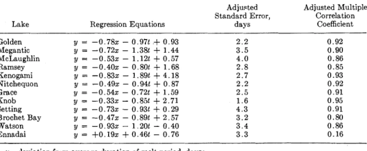
Regression equations calculated for each lake, standard errors, and correlation coefficients ad- justed for length of record [Ezekiel, 19531 are shown in Table 5. All correlations are signifi- cant a t t h e 0.05 level [Wishart, 19281 with the exception of those for Ennadai. T h e duration of the melt period of this lake appears t o be independent of both t h e date on which melt starts and the air temperature.
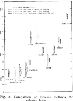
Standard errors for the regression equation method are compared in Figure 3 with standard deviations for the melting degree day method
TABLE 5. Regression Equations, Standard Error, and Correlation Coefficients
Lake
Adjusted Adjusted Multiple Standard Error, Correlation
Regression Equations days Coefficient
Golden y = -0.782
-
0.97t.+
0.93 2 . 2 0.92 Megantic y = -0.72s - 1.3%+
1.44 3.5 0.90 McLaughlin y = -0.532-
1.12t+
0.57 4 . 0 0.86 Ramsey y = -0.402-
0.80t+
1.68 2 . 8 0.85 Kenogami y = -0.832-
1.89t+
4.18 2.7 0.93 Nitchequon y = -0.492 - 0.94t+
0.87 2.2 0.92 Grace y = -0.542 - 0.72t+
1.59 2.5 0.91 Knob y = -0.332-
0.8%+
2.71 1 . 6 0.95 Setting y = -0.732-
0.93t+
0.29 4 . 3 0.91 Brochet Bay y = -0.472 - 0.89t+
2.57 3.2 0.80 Watson y = -0.932-
1.20t-
0.40 3 . 4 0.86 Ennadai y = +0.19x+
0.46t-
0.76 3 . 3 0.16y, deviation from average duration of melt period, days; 2, deviation from average date of start of melt period,"days;
Ice B ~ e a k u p 329
Fig. 3. Comparison of forecast methods for selected lakes.
and standard deviations of breakup dates. For some lakes, t h e results are excellent; for others, standard errors are not much less than t h e standard deviations of breakup dates. For example, t h e standard deviations for breakup dates for Nitchequon and Knob Lakes are 8.3 and 7.9 days; these are much greater t h a n the standard errors of 2.2 and 1.6 days of the regression equations. T h e standard deviation of breakup dates for Watson and Setting Lakes are, however, 4.4 and 5.3 days, just slightly more than standard errors of 3.4 and 4.3 indi-
cated by the regression equations. Standard er- rors for many of t h e lakes could probably be reduced if other variables affecting breakup (wind, ice thickness, and snow cover) could be introduced into the regresion equations. There were not enough d a t a available on these vari- ables, however, t o justify further calculations. All t h a t can be attempted is a qualitative dis- cussion of their relative importance.
T h e information t h a t was available demon- strated the effect of wind on breakup. An analy- sis of available wind records showed that i n 15 of 19 cases for which breakup was a t least 3 days later than forecast, t h e 24-hour wind speed on t h e day of breakup was below t h e monthly average. I n 15 of 23 cases for which breakup was a t least 3 days earlier t h a n fore- cast, wind speed was above t h e monthly average on t h e day of breakup. At Knob Lake, where wind effects are minimal, the standard error of estimate was 1.6 days; a t Watson Lake, where according t o the local observer wind always affects t h e clearing of ice from the lake, it was 3.4 days. Lakes with potentially long fetches, such as Setting and Megantic, had relatively large standard errors of 4.3 and 3.5 days, re- spectively.
T h e thickness of ice to be melted is another variable not considered in t h e regression equa- tions. T h e maximum ranged from 21-33 inches for Kenogami, 2 7 4 4 inches for Nitchequon, 35- 51 inches for Knob Lake, and 38-54 inches f o r Brochet Bay. T h e variation in t h e maximum from year t o year is so large t h a t appreciable errors in estimates of t h e date of breakup would be expected, if allowance were not made for it in regression equations. The results of t h e regression equation analysis indicate, however,
TABLE 6. Regression Equations Correlating z and y for Different Air Temperature Classifications during Melt Period
Air Temperature Regression Standard Correlation Number of
Classification Equation Error Coefficient Observations
Below average temperature,
-2.0°F or
>
y : -0.422+
4.4 3.1 0.68 35Average temperature,
-1.9
+
0+
1 . 9 " F y = -0 i3z+
0.9 3.8 0.75 58Above average temperature,
+2.0°F or
>
y = -0.fi3x-
4.2 4.0 0.85 58y, deviation from average duration of melt period;
330 G. P. WILLIAMS
t h a t ice thickness is not always so important a factor as one might assume. F o r example, the maximum ice thickness for Lake Ennadai varied from 48-90 inches; under comparable melting conditions, the number of days for ice to clear should show similar variation. The fact that t h e duration of the melt period of this lake is not highly variable suggests t h a t de- terioration of ice depends more on solar radia- tion and resultant 'candling' of ice than on ice thickness. T h e importance of ice thickness a s a factor affecting breakup date may vary from lake to lake, being especially important where ice covers a r e relatively thin.
Several other factors could contribute to re- gression equation errors, for example, variations in the amount of heat stored in the water under t h e ice, depth of snow cover, snowmelt runoff, a n d warm springs. Observation error would affect the reliability of the regression equations developed. I n addition, the shoreline- a r e s ratio is different for each lake, and this ratio affects the amount of heat t h a t can be advected from land surfaces [Scott, 19641.
GUIDELINES F O R FORECASTING BREAKUP
Records from the 12 stations were combined and used t o calculate three regression equations correlating y (as defined previously) with x
I I
- 20 I I I I
1
-I5 -10 - 5 0 + 5 4 1 0 115 + 2 0
D A Y S E A R L Y A V E R A G L D A Y S L A T E D C V I A T I O N S T A R 1 O F B R L A K U P . D A Y S
Fig. 4. Guideline for forecasting breakup date of continental lakes.
(also defined previously) for air temperature deviations classified as (1) below average air temperature (negative deviations -Z°F or greater), ( 2 ) average air temperature (devia- tions -l.g°F to + l . g ° F ) , and ( 3 ) above a ions average air temperature (positive devi t '
+2.0°F or greater). It was considered that these generalized equations would be useful for forecasting breakup dates when it is not pos- sible t o develop separate regression equations for individual lakes.
Table 6 shows regression equations developed for the three air temperature classifications. The correlations are significant a t the 0.05 level [Wishart, 19281. The standard error of esti- mate was 3.1 days for below average air tem- perature, 3.8 days for average air temperature, a n d 4.0 days for above average air tempera- ture. These equations were used t o develop t h e forecast guidelines plotted in convenient form on Figure 4. T h e only information needed for their use is average date of breakup, deviation from average date of s t a r t of breakup for the year in question, and a forecast air temperature. F o r example, if the start of breakup is 1 0 days late and the forecast air temperature is above average, the date of breakup should be about average. T h e forecast would be adjusted during the melt period if the actual air tem- perature were different from t h a t forecast.
T h e regression equations on which the fore- cast guidelines a r e based are significantly dif- ferent; consequently breakup forecasts based on above average and below average air tem- perature become increasingly different with changes in the start of significant melt. F o r example, if the date of start is 15 days early, there is only s difference of 7 days between fore- casts based on above average or below average air temperature. If t h e start is 20 days late, there is about a difference of 14 days between above and below average air temperature fore- casts. I t is difficult to give a sound physical interpretation of this result because the rate of ice decay depends on other parameters such as solar radiation, which may be indirectly re- lated to air temperature. Normally the amount of solar radiation available increases as breakup is delayed. The greater amounts of solar radia- tion would tend to be more effective in decaying ice a t above average t h a n a t below average air temperatures.
Ice Breakup I I I I I I I I I 1
-
L . ONATCHIWAY-
-
L . H A H 1 L . I C O Q C I 6 L.TEYlbCOUATA-
0 0-
-
A A-
0 0 - A 0 - =Ao0 0 a-
-
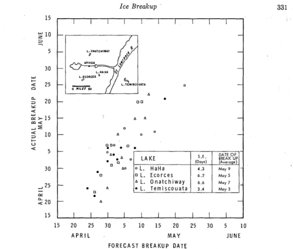
0 L. H a H a a o 0 L. E c o r c e s May 5 A L. O n a t c h i w a y-
a A L. T e r n i s c o u a t a MOY 3 0 a - A-
I I I I I I I I I I A P R I L M A Y JUNE F O R E C A S T B R E A K U P DATEFig. 5. Comparison of forecast date of breakup with actual date. The use and probable accuracy of these
forecast guidelines are illustrated by estimating breakup dates for four lakes within a 50- to 100-mile radius of a central meteorologic sta- tion in Arvida, Quebec. Deviations from aver- age date of start of breakup and air tempera- ture deviations during the active melt period were calculated for each year for which breakup records were available for analysis. The gen- eral equations in Figure 4 were used to obtain an estimated breakup date, which was compared with the actual breakup date (Figure 5 ) . The standard errors, ranging from 3.46.2 days, are quite reasonable when we consider that no information was available on local factors that might affect the date of breakup. I n practice, the accuracy of forecasts could be improved by a knowledge of local site conditions and by adjusting the forecast during the melt period for the air temperature, solar radiation, and wind conditions that actually prevail. These
forecast guidelines will necessarily be of limited accuracy, but they can be used particularly un- der abnormal conditions to give more objective guidance for estimating breakup dates than is now available.
DISCUSSION O F RESULTS
One of the major factors limiting the use- fulness of any method based on air tempera- ture records is the uncertainty in the forecast of air temperature during the melt period. The real problem of forecasting breakup dates is thus a part of the general problem of improv- ing short-term and long-term (30-day) forecasts of air temperature. Studies have been under way in the USSR for some time to improve long-range forecasting of breakup dates by relating air mass circulation to ice formation and breakup [Shz~lyakovskii, 19631.
Forecasts of weather conditions during the few days prior to breakup are especially im-
332 G. P. WILLIAMS
portant in determining the date ice will clear from a lake. Ice deterioration can be extremely slow during cool, cloudy weather, and a delay of several days in final breakup may result, even though all antecedent conditions favored early breakup. Above average solar radiation during the last few days of melt can result in rapid deterioration of ice covers, which when combined with strong winds can result in ex- tremely rapid clearing of ice from lakes.
T h e role of wind was assessed by analysis of the questionnaires circulated to observers who regularly record breakup for the Canadian Me- teorological Branch a t 54 lakes across Canada. On large lakes, wind almost invariably broke u p ice and drove it on t h e shore. T h e thick- ness of such sheet ice ranged from 1 4 feet, and the ice often piled u p to heights of 20 feet. For relatively small lakes with a fetch of 2-5 miles, ice from 1-2 feet thick was driven on shore but seldom piled up. I n only one case was ice driven on shore where the fetch was 1 mile or less.
T h e effect of wind depends not only on fetch but also on wind speed, direction, and duration
method of forecasting breakup date varies from lake to lake, being especially unsuitable for lakes where wind and river inflow have a dom- inant influence on breakup. Standard deviations calculated for several continental lakes ranged from 3.3-8.0 days.
Regression equations developed from past breakup and air temperature records make it possible to estimate breakup dates with a
standard error of 1 . 6 4 . 3 days, if the date of start of breakup and air temperature during the ice melting period are known. General guide- lines for forecasting breakup, developed from these equations, can be used when i t is not possible to calculate regression equations for a n individual lake. T h e equations and guidelines a r e suitable only for continental lakes where wind and river inflow effects are not dominant.
The accuracy of methods of forecasting breakup dates for lalce ice, based only on air temperature records, is limited b y many vari- ables difficult to allow for in regression equa- tions. T h e effect of wind is especially im- portant, particularly for lakes with e fetch greater than 1 mile.
and on the degree of ice deterioration when
Acknowledgments. The author acknowledges breakup occurs. These effects are to with gratitude the help of R , A, Armour with the ~ r e d i c t because there is uslially no information calculations and t l ~ e useful discussions with availebie on t h e degree of deterioration of ice ~everal other members of the Division of Bu~ld- covers immediately prior t o final breakup, and ing Rescarc.l~. This paper is a contribution from
the Division of Building Research, National often only limited informetion on wind speed, Research
Council of Canada and is
direction, and duration. with the a ~ n r o v a l of the Director of the Division. T h e nature of the problem of predicting
breakup dates for lake ice is such t h a t quite detailed information on the variables t h a t affect breakup would have to be available for each lake before a n accurate method of forecasting could be developed. A comprehensive manual on forecasting lake and river ice formation has been prepared in the USSR [Shulyakovskii, 19631 ; it is admitted, however, t h a t reliable methods for taking into account all the factors t h a t determine the destruction and thawing of ice have not yet been developed.
CONCLUSIONS
The date of lake ice breakup fluctuates within a rather wide range. The period between earliest and latest breakup dates is about 30-40 days for continental lakes and 50 days or more for coastal lakes (95% of the time).
T h e accuracy of the melting degree day
REFERENCES
Allen. W. T . R., Break-up nnd freeze-up dates in Cannda, 201 pp., Can. Dep. Transp., Meteorol. Br., Circ. 4116, Toronto, 1964.
Eriksson, J. V., The freeze-up and break-up of the ice in Swedish 1:lkrs (in Swedish), 95 pp.,
M e d d . Statens MeteoroL-Hydrogr. Anst., 1(2), 1920.
Ezekiel, M., Melho(1.s of Correlation Annlysis,
531 pp., John Wilcy. S e w Yorli, 1953.
Ragotzkie, R. A . , Compilation of freezing and thawing dates for lakes in north central United States and Canada. 61 pp., D e p . Meteorol. Tech. R e p . 3, University of Wis- consin, Madison, 1960.
Scott, J. T., A comparison of the heat balance of
lakes in winter, 138 pp., Dep. Meteorol. Tech. R e p . IS, University of Wisconsin, Madison, 1964. Shulyakovskii, L. G., Ed., Manual of Forecasting Ice Formation for Rivers and Inland Lakes, 245 pp., Israel Program for Scientific Tmnsla- tions, Jerusalem, 1966. (Original published in
Ice Breakup 333
Russian by Gidrometeorologicheskoe Izdatel' fresh-water lakes, pp. 203-215, Proc. Conf. Ice stvo, Leningrad, 1963.) Pressures Against Struct., Quebec, N o v . 1966,
Stankiewicz, M. J., Break-up can be foretold, Tech. Memo. 92, Associate Committee on Geo- Pulp and Pap. Mag., 48, 118-120, 1947. technical Research, National Research Council, Thomas, M. K., Some notes on the climatic his- Ottawa, 1968.
tory of the Great Lakes region, Proc. Entomol. Williams, G. P., A note on the break-up of lakes
Soc. Ontmrio, 99, 22-31, 1968. and rivers as indicators of climatic change, Williams, G. P., Correlating freeze-up and Atmosphere, 8, 23-24, 1970.
break-up with weather conditions, Can. Geo- Wishart, J., Table of significant values of the tech. J., 2( 4), 313-326, 19% multiple correlation coefficient, Quart. J. R o y . Williams, G. P., Ice-dusting experiments to in- Meteorol. Soc., 64,258, 1928.
crease the rate of melting of ice, 21 pp., N R C
9349, National Research Council of Canada,
Division of Building Research, Ottawa, 1967. (Manuscript received August 12, 1970;