A computational and experimental study of viscous flow around cavitating propulsors

(1)

A Computational and Experimental Study of

Viscous Flow Around Cavitating Propulsors

by

Wesley H. Brewer

B.S., University of Tennessee (1993)

Submitted to the Department of Ocean Engineering

in partial fulfillment of the requirements for the degree of

Master of Science in Ocean Engineering

at the

MASSACHUSETTS INSTITUTE OF TECHNOLOGY

June 1995

@ Massachusetts Institute of Technology 1995

Signature of Author

... j, 4V 'r ..

Department of Ocean Engineering

May 1995

OF TECHNOLOGY

DEC 0

8 1995

LIBRARIES

Certified by

... ... .. e....

ecturer

Accepted by....

Dr. Spyros A. Kinnas

and Principal Research Engineer

Thesis Supervisor

Professor

.

Doug

as Carmichael

Chairman, Departmental Committee on Graduate Students

(2)

A Computational and Experimental Study of Viscous Flow

Around Cavitating Propulsors

by

Wesley H. Brewer

Submitted to the Department of Ocean Engineering on May 1995, in partial fulfillment of the

requirements for the degree of Master of Science in Ocean Engineering

Abstract

A method for analyzing viscous flow around partially-cavitating and super-cavitating hydrofoils is presented. A nonlinear perturbation potential-based panel method is used to first solve the cavity solution in inviscid flow. A boundary layer solver is then applied on the surface bounded by the union of the foil and cavity surface. The effects of viscosity on lift and drag are studied for both partial and super-cavitating hydrofoils. Viscosity is shown to have a substantial effect in the condition of partial cavitation; on the other hand, minimal deviations from the inviscid solution are observed in the case of super-cavitation. Finally, the applicability of the present method to analyzing the viscous flow around cavitating propulsors is discussed.

Experiments are performed at the MIT Variable Pressure Water Tunnel to ultimately assess the validity of coupled inviscid/viscous cavity analysis method. Velocities are mea-sured along a rectangular control surface surrounding the hydrofoil, in the boundary layer region, as well as in the proximity of the cavity surface. The cavitation number is eval-uated by measuring the pressure inside the cavity via a manometer. The measurements are compared to the numerical results from the coupled, nonlinear, inviscid cavity anal-ysis method and a boundary layer solver. Forces are computed from measured velocities via momentum integrations and are compared with those predicted by the numerical method.

Thesis Supervisor: Dr. Spyros A. Kinnas

(3)

Acknowledgements

This thesis represents the work of which many people have contributed; I am very for-tunate to be working among such a talented group of people. I am gratefully indebted to Spyros Kinnas for more than generous amounts of encouragement, advice, and assis-tance. Dr. Kinnas' unselfish motivation to help students has granted me the opportunity to achieve many goals that otherwise would not have been possible. I would also like to thank Professor Drela for his assistance in adapting the viscous routines of XFOIL to cavitating flow. Also, much thanks goes to Professor Justin Kerwin for his excellent advice in times of need and to all those in the propeller group. I especially would like to express my appreciation to Shige Mishima, whose talented help in both academics and research was invaluable to the completion of this work. I am also grateful to my roommate Jesse Hong, for his expert advice on computers and for putting up with me over the years. Additional thanks go to our UROP'S Matt Knapp, Dianne Egnor, and Luke Sosnowski, for helping out in all phases of the experiment.

Most importantly I would like to thank my fiance Jenny, to whom I dedicate this thesis. Her constant love, devotion, and support has made graduate school much more fulfilling.

Much support also came from friends and family. A special thanks goes to my mother, for always believing in me. I could not have made it through college and graduate school without her substantial financial and emotional support. I also thank my dad for always inspiring me to the best and showing me a strong work ethic, and Michelle for always giving encouragement in times of need. Lastly, but most importantly, I would like to thank God who makes all things possible.

Funding for this research was provided by the Applied Hydromechanics Research pro-gram administered by the Office of Naval Research (contract: N00014-90-J-1086) and an International Consortium on Cavitation Performance of High Speed Propulsors composed of the following sixteen members: DTMB, OMC, Mercury, Volvo-Penta, IHI, Daewoo, El Pardo MB, HSVA, KaMeWa, Propellum, Rolla, Sulzer-Escher Wyss, Hyundai, Wartsila, and Ulstein.

(4)

Nomenclature

B bias limit

c chord

Cd dissipation coefficient = (1/peU3₎

_f

_r(au/Ir7)dr

I

CD drag coefficient = D/lpU c

Cf skin-friction coefficient = 27waIi/pu

CL lift coefficient = L/ pUc

Cp pressure coefficient = (P - Poo)/.pUl

CT shear stress coefficient = Tmax/pUe2

C0

EQ equilibrium shear stress coefficient

h mercury level in manometer

H shape factor = 6*/0

H" kinetic energy shape parameter = 0*/0

Hk kinematic shape parameter

= f[1 - (U/Ue)]d

7

+ f(U/Ue)[1

-

(u/Ue)]d?7

1 cavity length

n foil surface unit normal vector

Stransition disturbance amplification variable

N number of velocity samples

Pk measured cavity pressure

Pv vapor pressure of water

Poo free-stream pressure

P precision limit = tS

(8)

8

s arclength along foil surface

S, precision index of the mean = ao/v/-N

t coverage factor

tiax, maximum thickness of foil section

u, w horizontal and vertical velocities

U uncertainty estimate

Ue _{edge velocity}

Uoo free-stream velocity

x stream-wise distance

y vertical distance (analytical)

z vertical distance (experimental)

C angle of attack

6 boundary layer thickness

6:* _{boundary layer displacement thickness = f(1}_- _u/Ue)dy

0 boundary layer momentum thickness

= fU/Ue(1 -

/Ue)dy

0* _{kinetic energy thickness =}_f(u/ue)[1_{- u}2_/u2]dy

PHo2 water density

PiHg mercury density

PLIT leading edge radius of foil

cavitation number = (po - pv)/I~pU

uu _{standard deviation of horizontal velocity}

measurements

blowing source strength

total velocity potential = Din(x, y) + (x, y) perturbation potential

(9)

List of Tables

2.1 Testing cases and setup parameters at a free-stream velocity of 8 m/s (25

ft/s). . . . .. . . .... . . . . .. . 28

2.2 The bias limit, precision limit, and uncertainty estimate of the Flapping Foil Experiment performed at the MIT Water Tunnel (adjusted from Lurie

(1995)). ...

..

30

2.3 Heavy Foil Coordinates ... 34

3.1 Cavitation number and cavity volume from the analysis method, using

both predicted and experimentally observed cavity detachment as input. 52

4.1 Convergence of viscous cavity solution (a, V/c2, CL and CD) with number

of panels. Super-cavitating hydrofoil; r/c = 0.045, fo/c = 0.015, p = 0.85,

a = 30. . ... . . . .. . . 61

5.1 Comparison of lift and drag coefficients between experiment and theory.

a = 3.250 in fully-wetted flow (l/c=0). a = 3.50 in cavitating flow (10%,

20%, 30%, and 40%) ... ... 64

5.2 Cavitation number comparisons between experiment and theory, a =

3.250. (exp stands for experimental, p for differential pressure manometer,

ptun for tunnel pressure manometer, vel for velocity measurements, an for

(10)

List of Figures

1-1 History of code development for two-dimensional cavitating boundary layer

solver. ... .. 18

1-2 Hydrofoil with cavity and displacement thickness illustrating where bound-ary conditions are applied ... ... 19

2-1 Experimental setup in water tunnel showing foil and contour path of laser (all units given in millimeters). ... 23

2-2 Photographs of the hydrofoil in the water tunnel testing section. Top: l/c=0.10, bottom: l/c= 0.20. a = 3.50. ... 24

2-3 Photographs of the hydrofoil in the water tunnel testing section. Top: l/c=0.30, l/c=0.40. a = 3.50. ... 25

2-4 Horizontal velocity measurements on the top and bottom of a rectangular contour surrounding the hydrofoil with error bars showing plus or minus one-half standard deviation. ... 27

2-5 Example of boundary layer cuts near foil surface. a = 3.50 ... 27

2-6 Top and side view of hydrofoil, in tunnel testing section, showing the location of the pressure tap. ... 31

2-7 Manometer setup in water tunnel. . ... ... .. . . . . 32

2-8 Plot of foil surface ... 33

3-1 Hydrofoil with imposed boundary conditions ... 36

3-2 Hydrofoil with displaced body. Definition of main parameters. a = 3.50. _. ₃₈ 3-3 Flow of calculation method for solving viscous flow on a 2D partially-cavitating hydrofoil ... 41

(11)

LIST OF FIGURES

3-4 Flow of steps involved in coupled cavity analysis/boundary layer method. 45

3-5 Index arrangement for PCPAN, SCPAN, and CAV2D-BL. Indices

corre-spond to panel numbers (as opposed to node number). ... 47

3-6 Convergence characteristics of viscous cavity solution for CL, CD, a.is, and

V/c2 (cavity volume). a = 3.50,1/c = 0.30,N = the number of panels on

the foil and cavity. ... 50

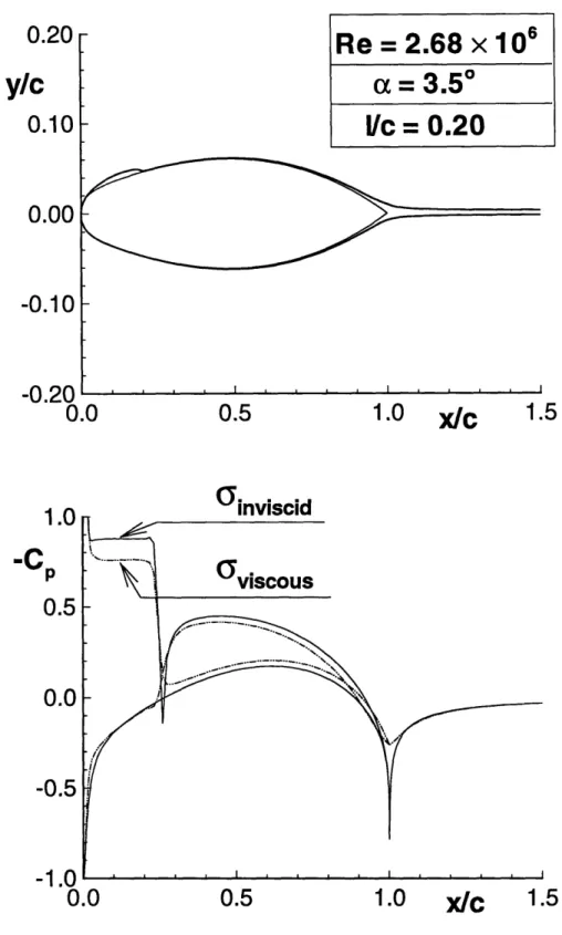
3-7 Above: Present method's prediction of heavy foil with viscous effects.

Below: Viscous and inviscid pressure distribution on foil. . ... 51

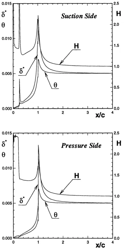
3-8 Displacement thickness, momentum thickness, and shape factor along

suc-tion and pressure sides of hydrofoil. a = 3.50,1/c = 0.20 . ... . 53

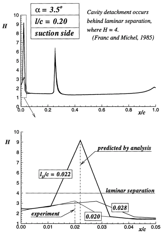
3-9 Shape factor along suction side of foil showing the method used to predict

cavity detachment. I/c = 0.20, a = 3.5. ... 54

3-10 Foil geometry and cavity shape showing the effect of tunnel walls. 'a=0.86 55 4-1 Super-cavitating hydrofoil in inviscid non-linear theory. Definition of main

parameters. Panel arrangement on the cavity and foil shown for N = 80. 57

4-2 The super-cavitating end parabola model where the kinematic boundary

condition is applied . ... 57

4-3 Super-cavitating hydrofoil with its boundary displacement thickness. . . 58

4-4 Super-cavitating hydrofoil in inviscid and viscous flow at Re = 2 x 107.

Cavity shape and boundary layer displacement thickness (top); pressure distributions (middle); and friction coefficient on the pressure side of the

foil and cavity (bottom). All predicted by the present method ... . 60

4-5 Cavity length, lift and drag coefficient versus cavitation number for a

super-cavitating hydrofoil at a = 1.50 (left) and a = 3.00 (right), in

invis-cid and viscous flow; predicted by the present method. ... 62

5-1 Above: the experimental lift coefficient versus the analytical model's pre-diction for the variety of cavity lengths. Below: the drag coefficient versus

(12)

LIST OF FIGURES

5-2 Velocity measurements along the normal to the cavity surface for cavity

lengths of 1/c = 0.10, 0.20. a = 3.250. (y = 0 corresponds to the cavity

surface location) .. .. .. ... .. .. .. .. ... .. .. .. .. ... . 68

5-3 Velocity measurements along the normal to the cavity surface for cavity

lengths of 1/c = 0.30,0.40. a = 3.250. (y = 0 corresponds to the cavity

surface location) .. .. .. ... .. .. .. .. ... .. .. .. .. ... . 69

5-4 Horizontal and vertical velocities along all sides of a rectangular contour

surrounding the hydrofoil.fully - wetted, a = 3.250... 71

surrounding the hydrofoil.l/c = 0.10, a = 3.5.. . ... . 72

surrounding the hydrofoil.l/c = 0.20, a = 3.5.. . ... . 73

surrounding the hydrofoil.1/c = 0.30, a = 3.50. . ... . 74

5-8 Top: Boundary layer profiles comparing experiment (circles) and theory (solid line), x/c = 0.50, fully-wetted, and a = 3.50. Middle: x/c = 0.80.

Bottom: x/c = 0.90. ... 75

5-9 Top: Boundary layer profiles comparing experiment (circles) and theory (solid line), x/c = 0.50, 1/c = 0.10 and a = 3.50. Middle: x/c = 0.80.

Bottom: x/c = 0.90. ... 76

5-10 Top: Boundary layer profiles comparing experiment (circles) and theory (solid line), x/c = 0.50, 1/c = 0.20 and a = 3.50. Middle: x/c = 0.80.

Bottom : x/c = 0.90. ... ... 77

5-11 Comparison of cavitation number (pressure coefficient in fully-wetted flow)

between experiment and theory for various cavity lengths. a = 3.250. . . 79

6-1 Top: the current viscous cavity model showing the momentum thickness

along the foil and wake surface. Bottom: the current model with the proposed jump model. ...

(13)

-LIST OF FIGURES

6-2 Top: preliminary results of the proposed jump model showing the mo-mentum thickness along the suction side of the foil and wake. Bottom:

velocity profiles showing trends of increasing momentum thickness... . 86

A-1 A 1 - 2 mm gap in measuring exists between the foil and the closest point

measured. ... 91

A-2 Above: The present method fit to a boundary layer profile. Below, result-ing displacement thickness from present method (shown as a diamond) as

well as viscous flow model's displacement thickness prediction. ... . 93

C-1 Experimental velocity measurements in the boundary layer region. a =

1.660,fully - wetted ... ... 97 C-2 Experimental velocity measurements in the boundary layer region. a =

0.70, fully - wetted. ... 98

C-3 Experimental velocity measurements in the boundary layer region. a =

1.660, 10%cavity. ... 99

1.660, 20%cavity. ... 99

0.40, fully - wetted. ... 100

D-1 Left: the inviscid cavity model with 10% cavity and a = 0.70. Right: the

corresponding pressure distribution. (10% 20% (1.660), 10% (0.70)) . . . 103

D-2 Left: the inviscid model's versatility allows the prediction of two cavities.

10% and 25% cavities a = 0.40 Right: corresponding pressure distribution. 104

D-3 Velocity profiles for both experimental and analytical showing the effect of transition location on the boundary layer. The measured profile has been

arbitrarily shifted vertically due to the ambiguity in the foil surface. . . . 104

D-4 Prediction of velocity profile in wake for various (pressure-side) transition

locations. a = 1.660, fully - wetted ... 105

D-5 Velocity profile comparisons between experiment and viscous model ... 106

(14)

LIST OF FIGURES

D-7 Lift and drag coefficients as a function of transition location,

sure side of the foil. Fully-wetted, a = 0.70. ...

sure side of the foil. Cavity flow, a = 1.660, 1/c = 0.20. . . .

sure side of the foil. Cavity flow, a = 0.40, 1/c = 0.45...

on the on the on the pres-107 108 109

(15)

Chapter 1 Introduction

Cavitation is the manifestation of vapor pockets in a flowing liquid owing to a local minimization of pressure. This phenomenon of liquid vaporization has antagonized the design of propulsors by causing:

* diminished efficiency/performance

* excessive structural vibration (leading to failure)

* immense material corrosion due to the high forces involved in the bubble collapse * flow noise

Cavitation is inevitably an issue in the design of efficient high speed pumps and propellers. Therefore, there is a great interest in studying the physics underlying the nature of cavitation. Research on cavitation was initiated in pursuit of developing methods to

control cavitation: methods to design more efficient hydrofoils and propellers that use

cavitation to their benefit.

In fact, optimally-cavitating propulsors can be more efficient than those designed to not cavitate. The presence of the cavity introduces the advantageous quality of having smaller viscous losses. However, it also introduces undesirable form drag, called cavity

drag. Thus, the design of the most efficient propulsor represents a delicate balance

(16)

1.1 Research History

viscous losses) or fully-cavitating (small blade area with minimal viscous losses but with cavity drag).

Computational tools have been of paramount importance in designing cavitating propulsors. These tools are developed in a systematic manner, starting with simple two-dimensional geometries in inviscid flow, working towards three-dimensional geome-tries in viscous flow. The philosophy underlying the development of the codes is to begin with the simplest model and progressively extend this model to more complicated and realistic flows. This work represents a small contribution in the efforts to ultimately develop an automated numerical method for the design of optimum propulsors.

This thesis attempts to address the issue of viscosity in cavitating flow. The effect of viscosity is studied by performing experiments on simple two-dimensional hydrofoils in cavitating flow. Knowledge obtained from experiments is then used to further de-velop existing computational methods to accurately model viscous flow around cavitating propulsors.

1.1 Research History

1.1.1 Experiments

Experimentation is an essential element in the study of cavitation. It is primarily useful for understanding the actual physics and details of the flow. A vast number of experiments have been conducted to investigate cavitation. The purpose in many of these experiments was to measure the lift, drag, and moment coefficients for various cavitation numbers. Parkin (1958) measured lift, drag, and pitching moment in cavitating and fully-wetted flow for flat plate and circular-arc sections. Meijer (1959) measured forces as well as pressures in the vicinity of the cavity trailing edge of a partially-cavitating hydrofoil. His experiments indicated essential differences between partially-cavitating and super-cavitating flows. Wade and Acosta (1966) studied the lift and drag on a plano-convex foil in the presence of partial and super cavitation. They also observed strong, periodic oscillations in both cavity length and forces acting on the hydrofoil. A secondary effort of

(17)

1.1 Research History

their experiments was to observe the formation and development of the cavity. Uhlman and Jiang (1977) studied the cavity length, for various cavitation numbers, on a plano-convex foil. There results were correlated to the theories of Wade (1967) and Geurst (1959). Maixner (1977) investigated the influence on wall effects on force and moment coefficients of a super-cavitating hydrofoil. His results were compared to the methods of Wu, Whitney, and Lin (1971).

Laser Doppler Velocimetry (LDV) measurements in the boundary layer, behind the cavity of a partially-cavitating hydrofoil, were performed by Kato et al (1987) and Fine (1988). Kato reported an appreciable increase in the boundary layer thickness due to the existence of cavitation. Kato also measured the unsteady flow in the presence of cloud cavitation using a conditional sampling technique. Lurie(1993) measured the formation of the unsteady boundary layer on a fully-wetted hydrofoil subject to sinusoidal gust (the

Flapping Foil Experiment), in addition to unsteady pressures on the foil surface.

Kinnas and Mazel (1993) performed LDV measurements about a super-cavitating hydrofoil. They measured velocities near the cavity surface to calculate the cavitation number. Measurements were also made along a rectangular contour surrounding the foil and cavity. These measurements were used with momentum integrations to calculate the lift and drag forces acting on the hydrofoil. A list of earlier super-cavitating experiments is given in Kinnas and Mazel (1993).

1.1.2 Numerical Methods

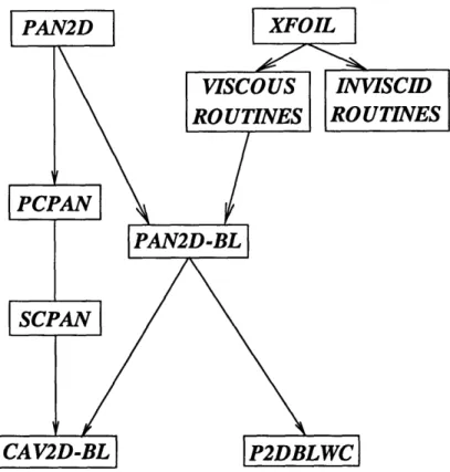
Many codes have been developed over the past few years to aid the designer in developing optimal blade geometries. A history of numerical methods used to model sheet cavitation is given in Villeneuve (1993). The nonlinear perturbation potential method by Kinnas and Fine (1990) laid the groundwork for the viscous cavity model, P2DBLWC.

Villeneuve's viscous cavity analysis method was based on Drela's (1989) airfoil anal-ysis code, XFOIL, which uses an interactive viscous-inviscid approach to solving the flow around airfoils. Drela's work was further developed by Hufford (1992) who applied the boundary layer method in a strip-wise sense to analyze the viscous flow around three-dimensional propeller blades. In doing this, Hufford coupled the viscous routines of

(18)

1.1 Research History

Figure 1-1: History of code development for two-dimensional cavitating boundary layer solver.

XFOIL to the inviscid perturbation potential method of PAN2D.1 The history of the

code is illustrated in Figure 1-1.

The scope of Villeneuve's work was divided into two strands: numerical and exper-imental. The numerical method, P2DBLWC, was based on Hufford's code, PAN2D-BL. To model the cavity, Villeneuve used a similar method to that used in boundary layer theory, where blowing sources were used to represent the cavity. This method is referred to as the "thin" cavity method, in which case both the cavity and the displace-ment thickness are assumed to be "small" with respect to the cavity length. Villeneuve's work also included the implementation of the method of images to account for the effects of tunnel walls.

To validate P2DBLWC, Villeneuve performed experiments on a partially-cavitating hydrofoil. In correlating experimental results with numerical predictions, he compared

(19)

1.2 Objectives

P2DBLWC: 'Thin" cavity approach CAV2D-BL: Nonlinear cavity approach

_. _ C•f--A* n--n

'-I-',,F

Figure 1-2: Hydrofoil with cavity and displacement thickness illustrating where boundary conditions are applied.

integral parameters, such as the boundary layer displacement and momentum thickness, as well as lift and drag coefficients. The predicted results by the analysis method were shown to be in good agreement with the experimental results.

1.2 Objectives

This thesis serves to continue Villeneuve's efforts to model viscous flow around cavitat-ing hydrofoils. Instead of comparcavitat-ing integral parameters, such as the boundary layer displacement and momentum thickness (as Villeneuve did), the results herein compare actual velocities, which are predicted anywhere in the flowfield, with those from experi-ments. In doing this, a numerical method was developed to extract velocity profiles from the integral quantities given as a result of the boundary layer solver.

The secondary goal of this work lies in further developing the code P2DBLWC: increasing the versatility and robustness of the boundary layer solver used to model viscous cavitating hydrofoils.

To this end, the following improvements were made to P2DBLWC:

* The non-linear cavity method: The boundary layer is solved on the cavity surface

resulting from "fully" non-linear cavity analysis.

* Implement a new spacing technique, blended spacing, which allows the user to spec-ify the cavity detachment location exactly and ensures continuous panel spacing.

(20)

1.2 Objectives

* Extend the method to super-cavitating sections. * Fix bugs in the old code.

* Formulate and implement the "momentum jump" model which models the in-creased momentum and displacement thickness which occurs at the trailing edge of the cavity (as evidenced by experiments).

Villeneuve's "thin" cavity method, P2DBLWC, has been shown to work well when the cavity is very thin compared to the foil thickness. In his method, he represents the cavity and boundary layer by using blowing sources applied on the cavity surface as shown in Figure 1-2. In this thesis, however, a different approach is used to model the viscous flow around the cavity, namely, the nonlinear cavity approach, as shown in Figure 1-2. First, the cavity is generated in nonlinear theory, then the boundary conditions are applied on the boundary surrounding the union of the cavity and foil surface. However, the present method does not ensure that the dynamic boundary condition, requiring the pressure to be constant on the cavity surface, is completely satisfied. The present method

only performs the first iteration of the inviscid/viscous coupling procedure. Kinnas et al (1994) performed a second iteration of the present method, which showed not the affect the results drastically.

The code incorporating these changes has been named CAV2D-BL - a two-dimensional

cavitating boundary layer solver.

(21)

Chapter 2 Experiment

The purpose of the partially-cavitating hydrofoil experiments (PACHE) is to acquire data which can be used to validate the coupled nonlinear cavity analysis method (PCPAN) and boundary layer solver (CAV2D-BL). Also of interest in these experiments is the study of how the cavity drag manifests itself into the wake. To fulfill these goals, velocity measurements and pressure measurements (cavitation numbers) were taken for various angles of attack and cavitation numbers.

PACHE was performed in three phases. The subsequent phases were necessary to fix problems in the previous phases. The following outline describes each phase of the experiment:

* Phase I:

- Performed by: Shige Mishima, Cedric Savineau, Wesley Brewer, and Platon

Velonias

- Problems:

* Fiber-optic beam was not working. Boundary layer measurements could

only be taken with horizontal component of laser.

* No turbulator strip on pressure side of foil introduced error in the

predic-tion of the transipredic-tion locapredic-tion.

(22)

2.1 Setup

- Performed by: Wesley Brewer

- Corrections since phase I:

* Fiber-optic beam fixed.

* Turbulator strip placed on pressure side of foil.

- Phase II problems: Pressure measurements could not be taken because

manome-ter was not working correctly. * Phase III:

- Performed by: Wesley Brewer

- Corrections since phase II: Manometer fixed

- Phase III Problems: Manometer still not completely accurate.

2.1 Setup

The experiments were performed in the MIT Variable Pressure Water Tunnel (Kerwin, 1992). The tunnel has a twenty inch square testing cross-section enveloped on all sides by plexiglass windows. First, the tunnel was de-aired at low speeds using the vacuum pump; then, the pressure was dropped below the point of cavitation inception. One impeller, driven by a 75 horsepower motor, propels the water through the closed-loop tunnel at speeds up to 9 m/s (30 ft/s); a speed of 8 m/s (25 ft/s) was used for this experiment.

Figure 2-1 shows the experimental setup. The foil, a "heavy" symmetrical stainless-steel foil, has a chord of twelve inches and a span of twenty inches. The maximum thickness to chord ratio is twelve percent at half-chord. A turbulator strip was placed on the pressure side of the foil at 1/5 chord. Two rubber gaskets, squeezed in between the plexiglass window and the foil, served to prevent any secondary flow between the pressure and suction side. The foil was mounted on the vertical plexi-glass walls at two points on each side, as shown in Figure 2-1. A stainless-steel pin, set at approximately 3/4 chord, was used to adjust the angle of attack.

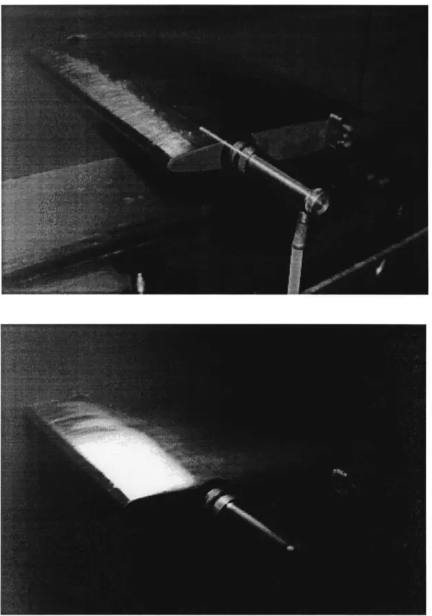
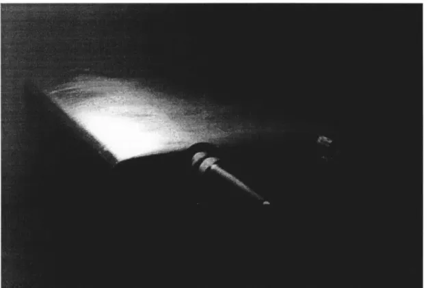
Figure 2-3 shows actual photographs of the cavitating hydrofoil in the testing section of the water tunnel. The top photo shows a very stable sheet cavity of extent 10%

(23)

2.2 Velocity Measurements U. 254 2. w

U

_z

xi

160 c = 305 165

Figure 2-1: Experimental setup in water tunnel showing foil and contour path of laser (all units given in millimeters).

of the chord length. It is evident that the "clean appearance" of the cavity becomes worse for larger cavity lengths. The measurements also confirm that the amount of uncertainty increases with increasing cavity extent. Notice that the cavity detachment

point is very pronounced in Figure 2-3, and very two-dimensional - an extremely desirable

characteristic in studying cavity detachment location.

2.2 Velocity Measurements

The present section discusses issues related to the acquisition of velocities in the flow-field. A description of the method used in taking velocity measurements is first presented, followed by an analysis of the errors involved in the measurement process. A complete set of the measurements may be found in later sections, where they are compared to results of the analysis.

2.2.1 Procedure

Velocities can be taken instantaneously anywhere in the flow-field using the TSI model 9533 Argon Ion Laser Doppler Velocimeter (LDV). The crossing of two monochromatic

mm

11~·1~·1~111111·1·1111·111~

(24)

2.2 Velocity Measurements

Figure 2-2: Photographs of the hydrofoil in the water tunnel testing section. Top:

(25)

Figure 2-3: Photographs of the hydrofoil in the water tunnel testing section. Top:

(26)

beams creates an interference fringe pattern. Seed particles' in the flow create a distur-bance in the fringe pattern; this disturdistur-bance is measured by a photodetector and then processed through digital signal analyzers, ultimately resulting in a velocity reading. A two-component optical laser was used in all phases of the experiment to measure velocities along the rectangular contour. In Phase I of the experiment, boundary layer velocities were acquired by the horizontal component of the laser (which cannot measure velocities

within 1 - 3 mm of the foil surface). However in Phase II, boundary layer measurements

were taken by a rotatable fiber-optic beam which measured velocities parallel to the foil

surface.

At each data point, the LDV takes a user-specified number of samples, in this case 500. Velocities are rejected if they are greater than three standard deviations from the mean; the standard deviation and mean are recomputed with the reduced data set (Kinnas and Mazel, 1993). Figure 2-4 shows a representative set of "good" data with error bars attached. The error bars represent plus or minus a half standard deviation from the stream-wise velocity mean (solid line). The standard deviations ranged from approximately three percent in inviscid regions up to ten percent in viscous regions and near the cavity. In some unusual situations the measured velocity had a standard deviation which was in the order of twenty percent or more of the mean value.

Velocities were measured in the proximity of the cavity surface as well as in the boundary layer region behind the cavity, and along the sides of a box which surrounds the hydrofoil as shown in Figures 2-1 and 2-5. Table 2.1 not only lists the setup for each testing case, but also the observed cavity detachment and reattachment points, or cavity leading and trailing edges respectively.

The free-stream velocity, U,,, is measured using a differential pressure cell far up-stream of the hydrofoil. All velocity measurements are normalized on its respective instantaneous free-stream velocity. Typically, the free-stream velocity will drift, up to five percent, over the course of the experiment.

(27)

1.4 u/U

1.2

1.0

0.8

0.6 -C

I I I I

I height of bars = 1 standard deviation) I

0.0

0.5

1.0 xIc

Figure 2-4: Horizontal velocity measurements on the top and bottom of a rectangular contour surrounding the hydrofoil with error bars showing plus or minus one-half standard deviation.

z/c

I

Figure 2-5: Example of boundary layer cuts near foil surface. a = 3.50

(28)

Table 2.1: ft/s).

Testing cases and setup parameters at a free-stream velocity of 8 m/s (25

Phase a

l1/c

Cavity L.E. Cavity T.E. Measurement Type

I 0.4 0.0 - - Boundary layer/Contour 0.4 0.01/0.50 0.1/0.80 Contour 0.7 0.0 - - Boundary layer/Contour 0.1 0.02 0.12 Contour 1.66 0.0 - - Boundary layer/Contour 0.1 0.02 0.11 Boundary layer/Contour 0.2 0.01 0.20 Boundary layer/Contour II 3.50 0.0 - - Boundary layer/Contour 0.1 0.02 0.20 Boundary layer/Contour 0.2 0.02 0.25 Boundary layer/Contour 0.3 0.02 0.32 Boundary layer/Contour 0.4 0.02 (0.4) Boundary layer/Contour III 3.250 0.0 - - Pressure/Contour 0.1 0.024 0.13 Pressure/Cavity velocity 0.2 0.025 0.24 Pressure/Cavity velocity 0.3 0.025 0.34 Pressure/Cavity velocity 0.4 0.021 0.47 Pressure/Cavity velocity _ _

(29)

2.2.2 Errors in Velocity Measurements

Errors in the velocity measurements, as measured by the standard deviations, are com-posed of: 1) errors due to the random fluctuations, or turbulence, in the tunnel, and 2) errors associated with variations the data acquisition equipment. The turbulence value of the MIT facility is approximately one percent of the free-stream velocity. The following quantities contribute to the total error associated with the LDV:

* repeatability of the coordinate system * variation of frequency shift

* calibration of the fringe spacing * calibration of the flow angularity

By propagating these individual errors through a Taylor series expansion, the total error associated with each component (stream-wise, vertical, fiber-optic) of the LDV can be determined. This was recently done by Lurie (1995) to find the error characteristics of the laser in the Flapping Foil Experiment (FFX), which was also performed at the

MIT Water Tunnel.

95% of the data should be expected to fall in a region, +/ - U, where U is the total

uncertainty of the data given by:

U = ,/B2 _{+ P2} _(2.1)

where B is the total bias limit of the propagated errors from each of the individual parameters listed above.

The precision limit, P, which is the range in which the mean of 95% of the data should fall, is defined as:

P = tS = (2.2) where S is the precision index and t is the coverage factor, equal to two for 95% coverage.

(30)

2.3 Pressure Measurements

Table 2.2: The bias limit, precision limit, and uncertainty estimate of the Flapping Foil Experiment performed at the MIT Water Tunnel (adjusted from Lurie (1995)).

Component B(m/s) P(m/s) U(m/s) U/Uoo

inviscid stream-wise 0.055 0.00029 0.058 0.8% vertical 0.061 0.00032 0.064 0.8% viscous stream-wise 0.134 0.00012 0.155 2.0% vertical 0.064 0.00041 0.101 1.3% fiber-optic 0.244 0.00244 0.256 3.4%

Table 2.2 lists the bias limit, precision limit, and total uncertainty estimate from data obtained in the FFX. The total uncertainty for the current experiment should be of the same order as those given in Table 2.2. In inviscid flow the uncertainty estimate should be very close to that of the FFX. On the other hand, due to the difference in the nature of

the two experiments,2 the error associated with the viscous velocities, in our experiment,

is less likely to be as high as that in the FFX.

2.3 Pressure Measurements

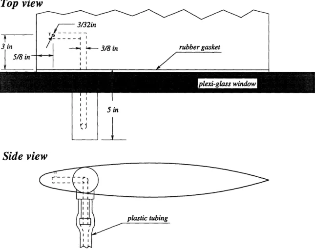
A manometer, shown in Figure 2-7, was used to measure the pressure on the suction side

of the foil, where a pressure tap was located at x/c = 0.05, as shown in Figure 2-6.

In the case of cavitating flow, problems were encountered with the phenomenon of water vaporizing in the manometer. To remedy this problem, the manometer was moved to a level much lower than that of the pressure tap. This added pressure to the top reservoir, shown in Figure 2-7, by the amount pHogAz, where Az is the increased

distance from the pressure tap to the manometer.

The following relation can be used to calculate the cavitation number or pressure coefficient on the foil.

(31)

2.3 Pressure Measurements

Top view

5 in

Side view

Figure 2-6: Top and side view of hydrofoil, in tunnel testing section, showing the location of the pressure tap.

(32)

2.4 Geometry of the Foil

Me

P

Figure 2-7: Manometer setup in water tunnel.

gh(pHg - PH20o)

o = -CP 1 PH

2PH20oo

(2.3)

where h is the height of the mercury level.

2.4 Geometry of the Foil

The foil used in the experiment has a zero-camber, symmetrical cross-section. Its geom-etry (originally unknown) was generated by first tracing the foil's section onto a piece of paper. From the trace on paper, the foil's thickness at many chordwise locations was measured. By fitting a fourth-order curve to those points, the following analytical expression for the foil thickness was derived, equation (2.4), in terms of the chordwise

location, x, from the leading edge of the foil3.

Y = cy. + C2X + C3 '1 5+ C4Y2

(2.4)

where Y = x/c, V = y/c and

3_{Notice that a different coordinate system, (x, y) shown in Figure 2-8, is used in the numerical results}

as opposed to the coordinate system used in the experiment, (x, z) shown in Figure 2-1.

b~d~a8n~

(33)

2.4 Geometry of the Foil f~ .d f~ U. IU

ylc

0.08

0.06

0.04

0.02

n 0n

' .0

0.2

0.4

0.6

0.8 X/C 1.0

Figure 2-8: Plot of foil surface.

cl = 0.1787

c2 = -0.3997

c3 = 0.7611

c4= -0.5401

Figure 2-8 shows both the measured foil offsets and the interpolated points from equation (2.4). Notice that the interpolation scheme smoothed out the uneveness in the measured surface offsets.

The foil has the following dimensions:

* c = 305mm (12in)

* PLEIC = 0.0160

* tmax/c = 0.120 at x/c = 0.485

with c being the chord, PLE being the leading edge radius, and tmax being the maximum

thickness of the foil. The foil thickness, near the leading edge, increases as the square root of the chordwise location. In particular, the first term on the right hand side of equation (2.4) determines the value of PLE, given by equation (2.5).

(34)

Table 2.3: Heavy Foil Coordinates x/c y/c x/c y/c 0.0000 0.0000 0.4000 0.0593 0.0050 0.0109 0.4500 0.0604 0.0075 0.0129 0.5000 0.0606 0.0125 0.0160 0.5500 0.0598 0.0250 0.0209 0.6000 0.0579 0.0500 0.0271 0.6500 0.0549 0.0750 0.0316 0.7000 0.0508 0.1000 0.0352 0.7500 0.0455 0.1500 0.0413 0.8000 0.0390 0.2000 0.0464 0.8500 0.0312 0.2500 0.0508 0.9000 0.0222 0.3000 0.0544 0.9500 0.0118 0.3500 0.0573 1.0000 0.0000 PLE = c

/2

Table 2.3 lists the foil offsets of the "heavy" foil.

2.4 Geometry of the Foil

(2.5)

(35)

I-Chapter 3

CAV2D-BL: Partially-Cavitating

Boundary Layer Solver

3.1 Formulation

3.1.1 Inviscid Cavitating Flow Theory

Assuming inviscid, irrotational, steady, uniform flow, in a field of infinite extent, the governing equation everywhere inside the fluid region is given by Laplace's equation:

V2D = 0 (3.1)

where 4 is the total velocity potential composed of the inflow potential, 4in, and the perturbation potential, q. Thus, the perturbation potential is defined as:

0(X,

y) =

#(x,

y) - i,n(X,

y)

(3.2)

In order to uniquely determine 0, the following boundary conditions, shown in Figure 3-1 are imposed (Kinnas and Fine, 1990):

* On the foil surface, the following kinematic boundary condition is applied, which requires the fluid flow to be tangent to the surface of the foil. Therefore,

(36)

P = PV =-U -n

Vý.<oo VO. -+ o

0

Figure 3-1: Hydrofoil with imposed boundary conditions.

S=-Uoo

n

on

where n is the surface unit normal vector.

* At infinity the perturbation velocities should go to zero.

V --+ 0 (3.4)

* The Kutta condition requires finite velocities at the trailing edge of the foil:

V¢

<

oo

_(3.5)

* The dynamic boundary condition specifies constant pressure on the cavity:

Iql

I

=

U00ooi

+

(3.6)

* Near the trailing edge of the cavity, a pressure recovery termination model replaces equation (3.6):

IqtI

=

Uoov /i+[1

- f(x)] 3.1 Formulation

(3.3)

U

=

(37)

3.1 Formulation

where f(x) is an algebraic function defined in Kinnas and Fine (1990) and the cavitation number, o0, is defined as:

poo - p,

Po-

-

P(3.8)

2

p0 is the pressure corresponding to a point in the free-stream and p, is the cavity pressure

(vapor pressure of water). The perturbation potential at a point P can be related to the potential on the foil surface and wake via Green's third identity:

erp = InR - dIn d -w ln R (3.9)

=

an

-n7

sw

where q is the perturbation potential on the foil, n is a unit vector normal to the foil surface, SB is the foil and cavity surface, Sw is the trailing wake surface, and R is the distance between a field point, P, and the point of integration over the foil or wake surface. c = 1 when P is on the foil or wake surface and e = 2 otherwise.

In the case of fully-wetted (non-cavitating) flow, the foil and wake is discretized into

N + Nw panels as shown in Figure 3-5, where N is the number of panels on the foil

surface and cavity and Nw is the number of panels on the trailing wake surface. The source and dipole strengths are assumed constant over each panel. On the foil surface, the source strengths, which are proportional to Oq/dn, are given by the kinematic boundary condition, equation (3.3). On the cavity, the dipole strengths, which are proportional to 0, are given from integrating the dynamic boundary condition, equation (3.6). The discretized version of Green's theorem results in a system of linear equations from which the perturbation potential can be solved for each panel on the foil and cavity.

In finding the cavity shape, the cavity length and the point of detachment are both given. The cavity height is determined in an iterative manner until both the kinematic and dynamic boundary conditions are satisfied on the cavity (Kinnas and Fine, 1993).

(38)

3.1 Formulation

U

0

Figure 3-2: Hydrofoil with displaced body. Definition of main parameters. a = 3.50.

3.1.2 Boundary Layer Theory

Near the foil, viscous effects are confined in the boundary layer. To account for these effects, blowing sources, of strength & are added to the foil surface.

d(Ue

*)

ds

(3.10)

where s is the arclength along the foil, U, is the velocity at the edge of the boundary

layer, and 8* is the displacement thickness.' Figure 3-2 shows the definition of the main parameters used in viscous theory. Given an inviscid edge velocity distribution, the following boundary layer equations are solved (Drela, 1989).

dO _{d + (H + 2) 0 d}a dUe

ds

U, ds

(3.11) 0 dH dH* 2_Cd _{C + (H} H* ds dH H* 2 0 dUe

Ue1)

ds

(3.12) (3.13)

'The displacement thickness is defined as the distance the streamlines are displaced due to the boundary layer: 6* = fo (1 - u/Ue) dy. For more information on this see Schlichting (1979).

dfi di~ dReo ds dReo ds

(39)

3.2 Numerical Implementation

_ dC,

f4.

Cy Hk__ 1 dUe

c

d,. = 5.6 V' C12] + 25 x [ ( ) 2 ] - (3.14)

Cr ds

[CrEQ

38*

2 6.7Hk

U, d

In the case of laminar flow, equations (3.11), (3.12), and (3.13) are solved for the quantities 6"*, 0, and hi. For turbulent flow, equations (3.11), (3.12), and (3.14) are solved

for the quantities 6*, 0, and C,.

The inviscid flow is coupled with the viscous flow via the wall transpiration model. This model gives the edge velocity at each panel in terms of the inviscid edge velocity

and a mass defect term, m = Ue *.2

Ue = U'"" + E{UeS*} (3.15) The boundary layer equations are solved first with the edge velocity distribution given from inviscid theory. Once 6* is found, Ue is updated via equation (3.15). The boundary layer equations are then solved again. This process continues until convergence is achieved.

This method is extended to partially-cavitating hydrofoils by ignoring the two-phase flow near the cavity surface, treating the fluid/vapor interface as constant-pressure, free streamlines, and forcing Cf to zero on the cavity surface (Villeneuve, 1993; Kinnas et al., 1994). The boundary layer equations are integrated over the non-linear cavity and foil surface.

3.2 Numerical Implementation

The details of the numerics used to model viscous flow around a partially-cavitating hydrofoil are given in the following three steps. Figure 3-3 illustrates the different stages involved in the calculation.

2_E

is a geometry-dependent operator, the discretized version of which is given in Section 3.2.2 (Huf-ford, 1990; Drela, 1989).

(40)

3.2 Numerical Implementation 40

3.2.1 Step 1: Calculate the cavity height (PCPAN)

Given a hydrofoil geometry, the first step is to calculate the cavity height. This is accomplished by running PCPAN, the partially-cavitating panel method, which solves for the inviscid cavity flow in non-linear theory (Kinnas and Fine, 1990).

In PCPAN, the user must specify the cavity leading and trailing edge. The method solves the inviscid flow in an iterative manner, by updating the cavity height until both the kinematic boundary condition and dynamic boundary condition are satisfied on the cavity. PCPAN gives as its result the cavity ordinates and the cavitation number.

3.2.2 Step 2: Calculate inviscid edge velocity on compound

foil (CAV2D-BL)

The next step involves using the loci of points which envelope both the cavity and foil surface, as shown in Figure 3-3, as a new foil: the "compound" foil.

Discretize Green's third identity, equation (3.9), into N panels to get (Hufford, 1990):

r = n - Dijgj - AAOWi (3.16) j=1 j=1 where D Jsf F

a

In R , Sij = In Rds

Wi

=

aInR

ds (3.17)

Dij is an influence function on i due to the jth dipole; Sij is an influence function on i

due to the jth source. Wij is the contribution of source strength from the wake and SCF

is the surface bounded by the union of the foil and cavity surface. The Kutta condition, equation (3.5), reduces to Morino's condition:

(41)

PCPAN

CAV2D-BL

Figure 3-3: Flow of calculation method for solving viscous flow on a 2D partially-cavitating hydrofoil.

Given Foil Geometry

"Compound Foil"

=

Foil + Cavity

(42)

3.2 Numerical Implementation

An, = ON - €1 (3.18)

Thus, equation (3.16) can be represented by the following set of algebraic equations:

... _DIN . DN-1,N DN2

-W1

-W 2 -WN 0 ...

0

W1

o

...

0 W2

0 ... 0 WN 0 S12 ... S21 • o

SNm

SN2

W D12 DiN DN-1,N DNi DN2

-W1

0 ... 0 W₁

o

...

0 W

2 - WN 0 ... 0 WN

and equation (3.19) simplifies to:

Ai¢j

= Sij

_-

'

O n

Therefore,

inv =

[A]-' [S]

an

and, from equation (3.2), the total inviscid potential becomes:

[inv] =

[4,l

[+inv]

The inviscid edge velocity can then be determined by numerical differentiation of equation

7r D₂₁ DN1 Let SiN SN-1,N 0

(3.19)

(3.20) (3.21)

(3.22)

(3.23)

-W2

(43)

(3.23) as such:

d18nv [₄ inv]+ - [sinv]i

e ds Si+1 _{- Si} (3.24)

3.2.3 Step 3: Solve the boundary layer equations on

com-pound foil (CAV2D-BL)

The inviscid edge velocity, Ui n_V, _{is used as the 0-th iteration for the viscous solution.}

Equation (3.35) is solved along with the boundary layer equations, equations (3.11), (3.12), and (3.13) for laminar flow and equations (3.11), (3.12), and (3.14) for turbulent flow. This closed set of coupled non-linear equations can then be solved using Newton's method.

[Ji

[SX]k

= - R , }k 1<i< N+Nw

where

and Jij is the viscous Jacobian given by:

0j jor ni or C,

S=

_ax-j

(3.25)

(3.26) (3.27)

Ri is the residual, the difference between the edge velocities of the kth iteration and the

k - 1 iteration:

R

•

_{= U}

,

_-

_Ue

- 1

_(3.28)

If the residual is below the user-specified value (EPS1), the iterations will stop. Other-wise, X is updated as follows:

(44)

[X]k

+

l = [X]k + [SX]k

(3.29)

The algorithm checks for excessive changes and underrelaxes the residual if it is higher than the accumulated root-mean-square change.

3.2.4 Step 4: Update the edge velocity (CAV2D-BL)

The effects of the boundary layer are modeled by adding blowing sources to the surface of the "compound" foil. In doing this, equation (3.16) becomes:

N j=1 N+NW j1 Bij j j=1

N j

¢.

j=1

(3.30)

where & is the blowing source strength given in equation (3.10) and B,, is an influence function, similar to Sai, representing the influence of i on the jth source and is given by:

Bi,

=

LSC

j

In Rds (3.31)

In matrix form, equation (3.30), becomes:

[A] [€] = [S]

rdlA1-

C1ra]an,,

•[]

+ [B] [61

(3.32) By multiplying the system by the inverse A matrix, and using equation (3.22):

[1] = [Iv] + [A]-

1 [B] [&]

From equation (3.2), the total potential 4 can be determined by:

[I] = [(•'v] + [A]-1 [B] [&]

(3.33)

(45)

Figure 3-4: Flow of steps involved in coupled cavity analysis/boundary layer method. Numerical differentiation of equation (3.34) with respect to the arclength s gives the edge velocity at the panel nodes:

Uk+1l U""n + j { Uv e* k _(3.35) Si+1 - Si where d d (3.36) S= [A]- 1 [B] (3.36)

ds

Figure 3-4 is a simple illustration of the flow from Steps 1 to 4.

3.2.5 Indexing of the panels

In coupling PCPAN and CAV2D-BL, careful steps must be taken in defining the regions where the boundary conditions are to be applied. The systems used in indexing the panels are defined differently in PCPAN than in CAV2D-BL as shown in Figure 3-5. In PCPAN, the panels are numbered clockwise, where the first index is at the trailing edge

(46)

3.2 Numerical Implementation 46

of the foil.

On the other hand, CAV2D-BL first searches for the stagnation point. The location of the stagnation point is placed in the center of the panel. On the suction side, the first index is the half-panel above the stagnation point; subsequent numbers follow clockwise. On the pressure side, the first index is the half-panel below the stagnation point; sub-sequent numbers follow counter-clockwise, as shown in Figure 3-5. In CAV2D-BL, the suction side of the foil is called side 1 (is=l) and the pressure side of the foil is side 2

(is=2).

The following quantities are used to specify the cavity location:

* NLE -number of panels between leading edge and cavity detachment (PCPAN)

* LCAV - cavity trailing edge node number (PCPAN)

* IBL - panel number index (CAV2D-BL)

* ICLES - cavity leading edge panel number, suction side (CAV2D-BL)

* ICLEP - cavity leading edge panel number, pressure side (CAV2D-BL)

* ICTE - cavity trailing edge panel number (CAV2D-BL)

These values are used to specify panels on which Cf must go to zero. Notice that the values given from PCPAN refer to the panel nodes while the values from CAV2D-BL refer to the actual panel and are related to NLE and LCAV given from PCPAN in the following manner.

The indices in PCPAN are related to those in CAV2D-BL by:

IBL = j (3.37)

ICLES = NLE + 1

(47)

PCPAN/SCPAN

INDEXING SYSTEM

CAV2D-BL

INDEXING SYSTEM

is=1 (side 1)

ICTE+1

is=2 (side 2)

Nw panels

panels

Figure 3-5: Index arrangement for PCPAN, SCPAN, and CAV2D-BL. Indices correspond to panel numbers (as opposed to node number).

re

I. I

I

1

(48)

j--3.3 Analytical Forces

For side 1:

nonzero 1 < j < ICLES

0 ICLES < j < ICTE

Cf = (3.38)

nonzero ICTE < j• N/2 + NSTAG

0 j > N/2 + NSTAG

For side 2:

i nonzero 1 < j < N/2 - NSTAG

0 j > N/2 - NSTAG (3.39) where N is the number of panels representing the compound foil and cavity surface,

NF is the number of panels on the pressure side of the foil surface, and NSTAG is the

number of panels shifted from the centerline of the leading edge.

3.3 Analytical Forces

The lift coefficient, corresponding to the coordinate system shown in Figure 3-2, is com-puted by taking the vertical component of the pressures integrated over the entire foil

surface. This expression is given by:

CL=

C

• nds

(3.40)

where C•p are the "viscous" pressures, or the pressures computed on the displaced foil surface as shown in Figure 3-7, and n, is the y-component of the unit normal vector.

The drag is composed of an inviscid and viscid contribution as such:

CD = Cn + C (3.41)

The inviscid term, C1Dv, is attributed to the drag of the cavity and is given by:

(49)

3.4 Convergence Characteristics

where Cr" are the inviscid pressures shown in Figure 3-7 and n, is the x-component of the unit normal vector. Cavity drag can be explained by attenuation of pressure near the trailing edge of the cavity, accurately modeled by the pressure recovery termination model, equation (3.7).

CyZ8 _{is the viscous drag term and is given by the "far-wake" approximation as (Drela,}

1989):

CDP = -(3.43)_c

where 0, is the momentum thickness computed far downstream,3 _{as shown in Figure}

3-2.

3.4 Convergence Characteristics

For 200 panels on a HP 9000/735 with a risc chip, the coupled PCPAN/CAV2D-BL took less than two minutes.

The convergence of the results of the viscous cavity solution with number of panels is shown in Figure 3-6. The inviscid solution converges much quicker than the viscous

solution. The viscous cavitation number, a"_,_{is not constant over the extent of the cavity,}

evident in Figure 3-7.

3.5 Results

An example of results from this method is shown in Figure 3-7. This shows the case of a 20% cavity at 3.5 degrees with the boundary displacement thickness superimposed on the foil and wake surface. Shown at the bottom of Figure 3-7 are the inviscid and viscous pressure distributions on the foil. Notice that viscosity largely affects the cavitation number. In addition, the pressure is not constant over the entire extent of the cavity anymore. From comparing the areas under the viscous and inviscid pressure distributions, we can also infer that the lift coefficient decreases due to the viscous effects.

3

A computational and experimental study of viscous flow around cavitating propulsors

A Computational and Experimental Study of

Viscous Flow Around Cavitating Propulsors

by

Wesley H. Brewer

B.S., University of Tennessee (1993)

Submitted to the Department of Ocean Engineering

in partial fulfillment of the requirements for the degree of

Master of Science in Ocean Engineering

at the

MASSACHUSETTS INSTITUTE OF TECHNOLOGY

June 1995

@ Massachusetts Institute of Technology 1995

Signature of Author

Department of Ocean Engineering

May 1995

DEC 0

8

1995

Certified by

ecturer

Accepted by....

Dr. Spyros A. Kinnas

and Principal Research Engineer

Thesis Supervisor

Professor

.

Doug

as Carmichael

Chairman, Departmental Committee on Graduate Students

A Computational and Experimental Study of Viscous Flow

Around Cavitating Propulsors

by

Wesley H. Brewer

Abstract

Acknowledgements

Contents

Nomenclature

f

= f[1 - (U/Ue)]d

+ f(U/Ue)[1

-

(u/Ue)]d?7

CONTENTS

8

= fU/Ue(1 -

/Ue)dy

List of Tables

(1995)). ...

..

30

List of Figures

Chapter 1

Introduction

1.1

Research History

1.1.1

Experiments

1.1.2

Numerical Methods

1.2

Objectives

Chapter 2

Experiment

2.1

Setup

U

z

xi

2.2

Velocity Measurements

2.2.1

Procedure

11~·1~·1~111111·1·1111·111~

1.4

u/U

1.2

1.0

0.8

0.6

_f

_z

_(3.5)