Complex materials handling and assembly systems.

COMPLEX MATERIALS HANDLING AND ASSEMBLY SYSTEMS

Final Report

June 1, 1976 to July 31, 1978

Volume II

Multicommodity Network Flow Optimization in Flexible Manufacturing Systems

by

Joseph Githu Kimemia and Stanley B. Gershwin

This report is based on the thesis of Joseph Githu Kimemia, submitted in partial fulfillment of the requirements of Master of Science at the Massachusetts Institute of Technology in January, 1979. Thesis supervisors were Dr. S. B. Gershwin, Lecturer, and Professor M. Athans, Department of Electrical Engineering and Computer Science. The research was carried out in the Laboratory for Information and

Decision Systems with partial support extended by National Science Foundation Grants NSF/RANN APR76-12036 and DAR78-17826.

Laboratory for Information and Decision Systems (formerly Electronic Systems Laboratory)

Massachusetts Institute of Technology Cambridge, MA 02139

optimization approach. Mathematical methods which exploit the structure of the problem to generate manufacturing strategies are outlined. Numerical results show that the method produces results which agree with intuition and simulation for two- and

four-workstation systems.

-1-gestions, and discussion. The contribution of the members of the Manufacturing Group at L.I.D.S., in particular John Ward for the CAN-Q results, G. Secco-Suardo and Konrad Hitz for discussion on the network of queues models and the scheduling problem, respectively, and Yehiam Horev for the simulation, is much appreciated.

In the work on the augmented Lagrange Multiplier algorithm,thanks go to Dr. Earl Barnes of I.B.M. for his help both in the theory and the coding of the algorithm. Comments made by Professor W. Maxwell of Cornell University are much appreciated.

Thanks finally go to Arthur Giordani for the drafting and the L.I.D.S. typists for their work in the preparation of the document.

-ii-ACKNOWLEDGEMENTS TABLE OF CONTENTS LIST OF FIGURES LIST OF TABLES

CHAPTER 1. INTRODUCTION

1.1 The Strategy Assignment Problem in Flexible

Manufacturing Systems 1

1.2 The Network Flow Optimization Approach 4

1.3 An Outline of the Report 5

CHAPTER 2. THE MODELLING OF FLEXIBLE MANUFACTURING SYSTEMS 7

2.1 Introduction 7

2.2 The Stochastic Model 8

2.2.1 Exact Solution of Network of Queues

Models 9

2.2.2 Approximate Methods for the Analysis of

Network of Queues Models 13

2.3 Modelling and Optimization of Flexible Manufacturing

Systems 16

2.3.1 Modelling of Systems with Stochastic Opera-tion Times

2.3.2 Modelling of Deterministic Systems 32 2.4 An Approximate Method for Finding the Production Rate

of Balanced Closed Systems

2.5 Some Characteristics of the Solutions of the

Optimization Problems 44

-iii-SYSTEMS 47

3.1 Introduction 47

3.2 Linear Programming and Flow Optimization in Flexible

Manufacturing Systems 47

3.3 Non Linear Programming in Flexible Manufacturing

Systems 51

3.4 Conclusion 63

CHAPTER 4. NUMERICAL RESULTS FOR TWO- AND FOUR-WORKSTATION

SYSTEMS 64

4.1 Introduction 64

4.2 Optimization Results for a Two-Workstation System 65 4.3 Results for a Four-Workstation Deterministic System 91

4.3.1 Five-Part Example with Strategies

Enumerated in Advance 91

4.3.2 A Scheduling Procedure for the Loading

Station 95

4.3.3 Six-Part Examples: Strategies not

Enumerated in Advance 100

4.4 Conclusion 106

CHAPTER 5. OPEN AREAS FOR FUTURE RESEARCH 110

5.1 Introduction 110

5.2 Reliability and Limited Capacity Constraints in

Flexible Manufacturing Systems 110

5.3 Application of Network Flow Optimization to

Strategic and Tactical Problems 115

5.4 Summary of Open Areas 119

CHAPTER 6. CONCLUSION AND SUMMARY 120

APPENDIX: The Closed Network of Queues Optimization Model Applied 122 to a Two-Workstation System

REFERENCES 127

-iv-1.2 Operational Requirements for a Machine Tool Chuck 3

2.1 An Example of a Workpiece 18

2.2 Graphical Representation of Strategies 22 2.3 Linear Arrangement of Workstations (Flexible

Transfer Line) 28

2.4 The Two Possible Strategies 28

2.5 A Flexible Manufacturing System 33

2.6 Approximate Expression for G(M,N-1)/(G(M,N) as a

Function of N. 43

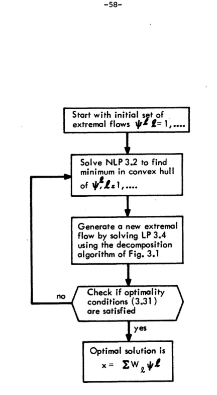
3.1 Flow Generating Decomposition Algorithm 52 3.2 Tree Flow Formulation of the Cantor-Gerla Extremal

Flow Algorithm 58

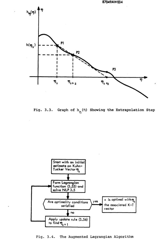
3.3 Graph of hn (n) Showing the Extrapolation Step 62

3.4 The Augmented Lagrangian Algorithm 62

4.1 A Two-Workstation System 66

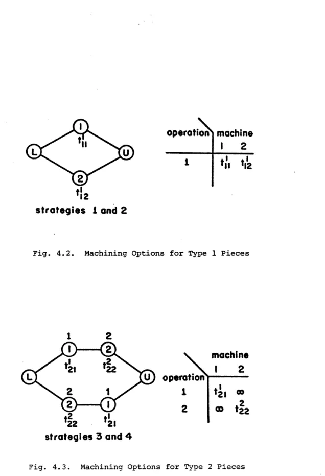
4.2 Machining Options for Type 1 Pieces 67

4.3 Machining Options for Type 2 Pieces 67

4.4 Optimal Mix as a Function of In-Process Inventory 71 4.5 Optimal Production Rate as a Function of In-Process 72

Inventory

4.6 Optimal Workstation Utilization as a Function of

In-Process Inventory 73

4.7 Optimal Average Queue Lengths as a Function of In-Process Inventory

4.9 Optimal Split X as a Function of pl 77 4.10 Optimal Workstation Utilizations as a Function

of l' With Q;10 78

4.11 Optimal Average Queue Lengths as a Function of P1' With Q=10

4.12 Production Rate as a Function of V1 with X as a Parameter.

82 4.13 Utilization of Workstation 1 as a Function of pi with X as 83

a Parameter.

4.14 Utilization of Workstation 2 as a Function of P1 with X as 84 a Parameter.

4.15 Optimal Workstation Utilization as a Function of .1 With 86

Q=OO.

4.16 Production Rate as a Function of X with V₁ as a Parameter.

4.17 Optimal Production Rates as Functions of 1 90₉₂

4.18 A 4-Workstation System 92

4.19 Production Rates for 4-Machine 5-Piece Example as a

Function of the Number of Pallets N. 98

4.20 Queue Occupation for 4-Machine 5-Piece System

4.21 Strategy Diagram for Type 2 Workpiece Six-Part Problem,

Example 1 104

4.22 Queue Occupation for 6-Piece System Example 1 107 4.23 Queue Occupation for 6 Piece System Example 2 108 5.1 Model of a Queueing System with Capacity Constraints 113 5.2 Closed Network of Queues Model for a Flexible

Manu-facturing System 113

-vi-A.2 Production Rate as a Function of X with I1 as the

Parameter 125

A.3 Utilization of Workstation 1 as a Function of 126

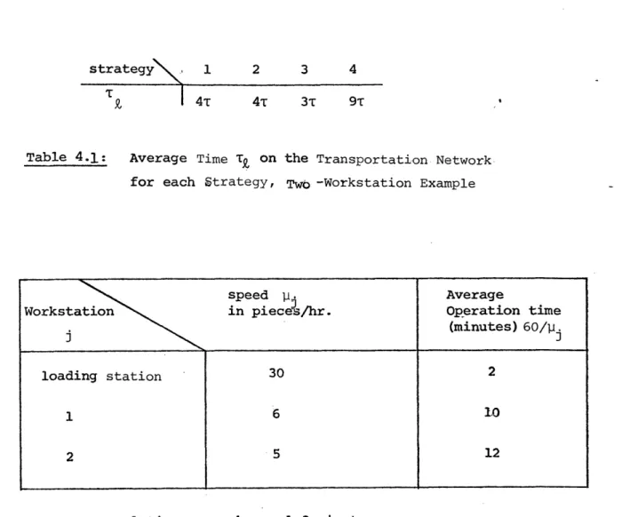
-vii-2.1 Machining Times t.. for Operations at the Workstations 20 on part i, the valve housing

2.2 Two Possible Strategies for the Manufacture of the Valve 21 4.1 Average Time TP on the Transportation Network for each

Strategy, Two-Workstation Example 68

4.2 System Parameters, Two-Workstation Example 68 4.3 Strategies and Optimal Splits for 4-Machine Case with

5 Part Types 93

4.4 Predicted and Simulation Utilization with 1st Priority

Routes Only and Using Optimal Splits 94 4.5 Predicted and Actual Production in 1500 Time Step Interval 94 4.6 t.. Matrices and Operation Requirements for 6-Part Example 101

13

4.7 Example 1: Optimal Strategy Assignments 102 4.8 Example 2: Optimal Strategy Assignments 103

k

4.9 Optimal Flow Rates x.. for Type 2 Piece (Six-Part Problem, 104 Example 1)

-viii-lines. In order to increase productivity in this sector of industry, flex-ible manufacturing systems are being designed and built.

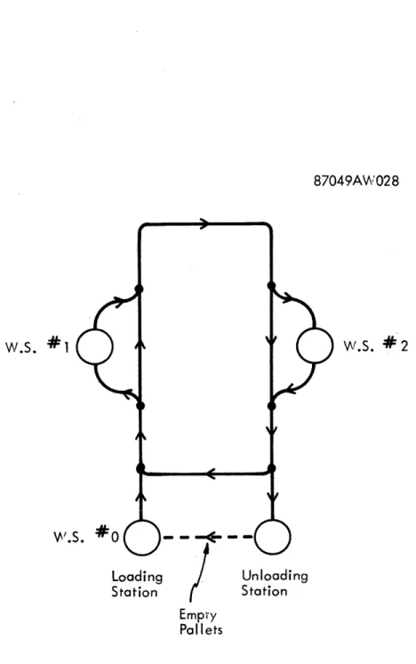
A flexible manufacturing system such as the one depicted in Fig. 1.1, consists of workstations capable of performing a number of different tasks,

interconnected by a transportation system. Workpieces are loaded onto pallets at a loading station, undergo a specified sequence of operations at the workstations, and then go to an-unloading station. The processes at the workstations are mostly automatic. At certain stations, like the

load-ing station for example, some manual operations may be performed (Hughes, 1977).

Several different kinds of pieces are manufactured simultaneously in the system. Each piece has a given number of operations necessary for its completion, as shown for example, in the piece of Fig. 1.2. There is a

choice in the system as to which workstation should perform each operation. Any entering workpiece therefore has the choice of several different routes or manufacturing strategies available. A strategy for each piece assigns

each operation to a workstation with the capability of performing that operation. The strategy also specifies the sequence of workstation visits.

In order to gain maximum output and utilization at minimum cost, the overall behavior of the system should be studied. Furthermore, mathematical models and algorithms are needed which will enable controllers to make

decisions affecting the system with minimum human intervention.

An important problem, which has a fundamental effect on the production rate and utilization of the system, is the assignment of strategies to the workpieces. Given a flexible manufacturing system with a specified production mix of pieces and given the locations at which all the operations can be

performed in the system, one wishes to pick the optimal steady-state mix of strategies for all of the pieces being produced.

-1-i

I I

I

I

I

§

S

. $ Z-IF'

} t E Zoo zzzf,/.o _{Ji~~~~~~~__} Alvue R AEu A ,p, ,

I

Extensive simulation studies of flexible manufacturing systems have been made (Hutchinson, 1977) (Horev et al., 1978) (Lenz and Talavage, 1977). They allow detailed investigation of the effects of parameter variation and strategy assignment on system performance.

Solberg (1977) and Ward (1980) model the system as a closed network of queues. Steady state results which are in good agreement with simulation results and observed performance of an actual system are obtained. The use of the closed network of queues model as an analytic method of strategy assignment has been suggested by Secco-Suardo (1978).

The machine or job shop problem has had considerable attention in the past and is in the class of combinatorial problems. They can be formulated and solved as 0-1 integer programming problems (Stern et al., 1977) (Fisher, 1970). In the case of a flow shop where the jobs must undergo a sequence of operations, the solution is difficult even for a three-machine system

(Kanellakis, 1978). A particular difficulty with this approach is that it makes an optimal schedule for a given number of jobs. What is required is a method of calculating optimal strategy assignments for a system that is operating continuously.

1.2 The Network Flow Optimization Approach

In this research, a network flow optimization approach is taken. Rather than analyze the movement of individual pieces through the system, the ag-gregated flow of pieces is analyzed. Network of queues models are used to account for congestion effects at the workstations.

Flow optimization techniques have been successfully applied to trans-portation and computer communication problems. In transtrans-portation systems, a frequently occuring problem is that of predicting traffic flows on a net-work of roads given travel demand between origin-destination pairs in the network. The solution is given by Wardrop's Principle; traffic distributes itself on the available routes in such a way that no single user can shorten his or her travel time or cost by using another route. For this reason it is often referred to as "user optimized flow" (Dafermos and Sparrow, 1969). A related problem but with a different solution is the system optimization

by data links as in the ARPA-network. Messages are routed from origins to destinations via intermediate computers. Each message experiences a random delay which is on the average a non-linear function of the flow rate (usually measured in bits per second) on a link. The objective is to route the

mes-sages in such a way that the total overall delay is minimized. This problem has been formulated and successfully solved as a non-linear network flow optimization problem (Frank and Chou, 1971).

Multi-commodity, minimum-cost, network flow optimization problems with resource constraints at network nodes have been examined by Wollmer (1972), Malek-Zavarei and Frisch (1971). Resource constrained problems occur, for example, in transportation problems with a limited number of vehicles or communication problems where there are capacity constraints at network nodes. Decomposition methods have been applied to solve such problems. The work-stations in flexible manufacturing systems can be viewed as scarce resources to be shared amongst all the types of pieces in the system. Similar methods can then be used to decompose the problem into easily solved sub-problems. 1.3 An Outline of the Report

The model is presented and the optimization problems formulated in Chapter 2. Systems having nondeterministic arrivals and processing times give rise to non-linear optimization problems. The production rate of the

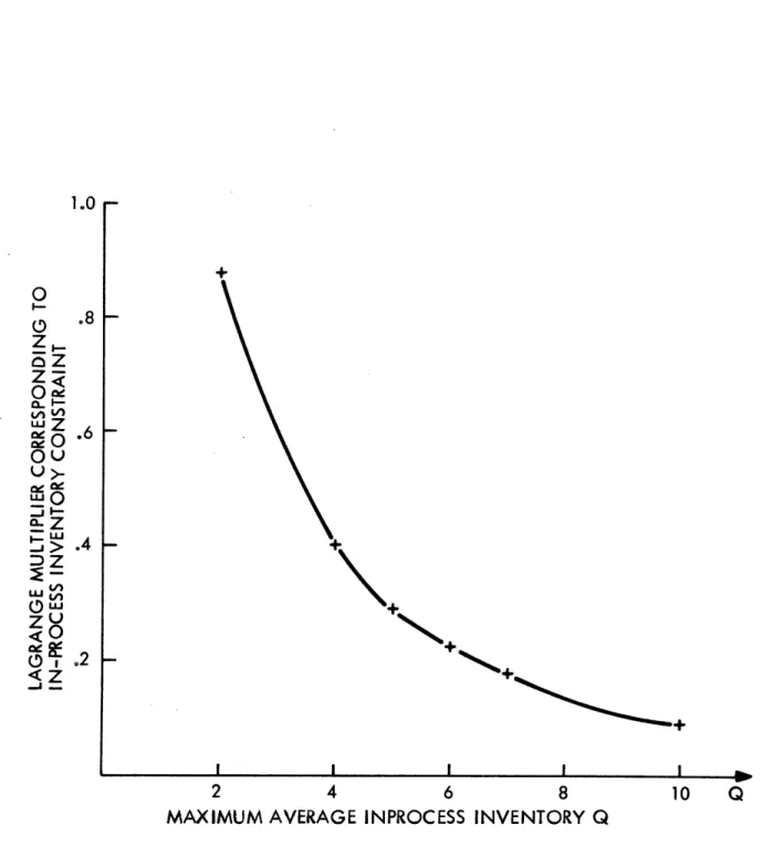
system should be maximized but the build up of queues within the system should be avoided. A price can be put on the average number of pieces within the system (the in-process inventory). Alternatively the inventory can be constrained to be below a certain given value. Deterministic systems, or systems in which the processing and interarrival times have a small

variance, give rise to linear programs. Asymptotic results for closed queue-ing network models (Gordon and Newell, 1967) (Secco-Suardo, 1978) and work rate theorems (Chang and Lavenberg, 1972) indicate that the linear programs

Chapter 3. Decomposition methods (Dantzig, 1963) are used to break linear programs into a set of strategy-generating minimum processing cost sub-problems each involving only one type of workpiece. Only a subset of all the possible manufacturing strategies are considered and they do not have to be enumerated in advance. A master problem finds the optimal combination of strategies for all the pieces.

An extremal flow algorithm (Cantor and Gerla, 1974) (Defenderfer, 1977) minimizes non-linear objective functions subject to linear constraints by

expressing the network flow rates as a convex combination of extremal flows. The extremal flows are generated by solving a linear program at each step. This method was originally developed for solving routing problems in packet switched computer networks (Cantor and Gerla, 1974) and has proven to be an effective method of obtaining the optimal routing in a network (Defenderfer, 1977). The Lagrange multiplier method of Hestenes (1969) and Powell (1968) converts a non-linearly constrained optimization problem into a series of problems where a non-linear Lagrangian function is minimized subject to the linear flow and resource conservation constraints. The extremal flow algo-rithm can then be used to minimize the Lagrangian function.

As an example of the application of the network flow approach to the strategy assignment problem, numerical results for a two- and four-work-station system are presented. The effect of changing some of the system parameters on the optimal strategy assignment, production rate and work-station utilization is investigated for the two-workwork-station system. The strategy assignments for the four-workstation system are implemented on a discrete simulation and the effects observed.

There are a number of outstanding problems for which analytic solution techniques would be extremely useful. Chapter 5 identifies problems for which network flow optimization appears to be promising as a component of a solution technique.

2. THE MODELLING OF FLEXIBLE MANUFACTURING SYSTEMS 2.1 Introduction

Accurate modelling of flexible manufacturing systems is important if an understanding of overall system behavior is to be gained. Of even greater importance is the building of models which will enable computers to make decisions either on- or off-line when running the system under automatic

control.

On a system-wide level, the static optimization problem is concerned with the steady state behavior of the system. The average values of utili-zation of the workstations, queue lengths at workstations, flow rates on the transportation links and the in-process inventory are of interest and define the state of the system.

Preliminary investigation is being carried out on small two- to four-workstation simulated systems. Practical systems will be much larger. The Sundstrand system at the Caterpiller plant at Peoria, Illinois, for

ex-ample has nine workstations, sixteen dual loading/unloading stations and produces two sizes of gear box casings, each consisting of two parts (Stecke, 1977). The size of the system gives rise to models with large numbers of variables. Care must be taken in keeping the dimension of the model to a minimum. In Section 2.2 flexible manufacturing systems are modelled as

networks of queues. Exact solution methods which have been applied to models of actual systems are surveyed. These methods are restricted to system

models which satisfy certain assumptions regarding service time distributions and arrival processes. Approximate methods are introduced for application to more general models. Optimization problems based on networks of queues are formulated in Section 2.3.1.

Section 2.3.2 formulates linear programming problems for systems whose service times are either deterministic or have small variances. In this case the non-linearities which account for the build up of queues are absent. The flow rates in the system are then the only variables of concern. Section 2.4 develops an approximation to the production rate of a balanced system with a finite number of pallets. Some aspects of the optimal solution of

2.2 The Stochastic Model

A network of queues consists of M nodes at which there are one or more servers. In a flexible manufacturing system these would correspond to the workstations and the loading and unloading stations. The service time at station i is taken to be a random variable with a known probability density function and mean l/ _{i .}* In a manufacturing system there are different types of workpieces each with its own service time distribution at each workstation. In most practical cases, the ratio of the numbers of different types of pieces being produced is specified.

It is assumed that once a workpiece leaves workstation i, it proceeds to workstation j with probability Pij. Workpieces originating from outside the system arrive at workstation i at a rate ai. The arrival process is stochastic with known statistical properties. The arrival rate X. at work-station j thus satisfies

M

-iX a.+ ' pij i (2.1)

i=l

The probability that a workpiece leaves the system after the completion of service at workstation i is simply 1 - P.

j=l 1

A network of queues is described as open if there are arrivals and departures to and from outside the network (Baskett et al., 1975). If, in

equation (2.1), a.0- and pi = 1 for all i, the system is closed. In this case there are N jobs circulating inside the network with none leaving and no fresh arrivals. The arrival rates X. then satisfy

M

j

il1

The matrix p=(pij) represents transitions in an underlying ergodic Markov chain (Baskett et al., 1975). With non-zero values of ai, (2.1) can be solved to give unique values of Xk. Equation (2.2) however, consists of self- consistent equations which can only be solved to within a multiplicative constant.

2.2.1 Exact Solution of Network of Queues Models

The open network was originally studied by Jackson (1963). The assump-tions made were that the service time distribution at all nodes is exponential and that the arrival process from outside the network is Poisson. It is also

assumed that there is only one class of customers. Under these assumptions and also given that there is unlimited queueing space at all the nodes, the system can be modelled as an infinite (but countable) state Markov process. Each state is defined by the vector k=(kl,k2, ..kM ) where ki is the number of customers either receiving or awaiting service at node i. Jackson's result is that the steady state limiting probability of being in any state k can be written in product form as

P(k) = Pl(kl)p2(k2)...PM(kM) (2.3)

Pi(ki) is the marginal probability of having ki customers at node i. The amazing thing is that Pi(ki) is identical to the steady state probability distribution of a single M/M/n queue. The implication of this result is that under the Poisson arrival, exponential service time assumptions, the variables ki are mutually independent in the steady state and thus each queue may be analyzed in isolation. Gordon and Newell (1967) derived the

steady state probability distribution for a closed network with N identical customers, and an exponential service time distribution at each of the M nodes. A finite state Markov model results. The number of states is equal

to ( N+M- 1 which is the number of ways that the N customers can be placed at the M nodes. A product form solution is again found with

1 M P(k) = G(M,N) i f. (ki) (2.4) i=l 1 M and I k = N (2.5)

_.--in which G(M,N) is a normaliz_.--ing constant. The functions fi(ki) satisfy the flow balance equations of the Markov chain model of the system. In this case there is strong interaction among the system nodes through the rela-tionship (2.5).

An important effect is the asymptotic behavior of a closed network of queues as the number of customers N inside the system grows without bound. Let x.i be an arbitrary solution to equation (2.2). If there are ri servers at station i, each with service rate pit the relative utilization ui of each workstation is defined as

x.

u. = (2.6)

There exists one or more stations with u = max u.. These stations are termed bottleneck stations (Gordon and Newell, 1967) for the closed network. It is shown that at any state for which k ,the number of customers at the bottleneck station,is finite,

li P(klk2,...kM) 0 (2.7

The marginal distribution PB(kl... k-l' ,k+ l' ...k) taken at all stations excluding the bottleneck stations is finite and well defined and takes the product form

M

PB (kl' k2...kM) = i(ki) (2.8)

i=l

ipB

where B is the set of bottleneck stations. Thus as the number of customers inside the network becomes large, the bottleneck stations act as generators of Poisson arrivals. The rest of the network behaves like an open network

(Secco-Suardo, 1978).

The analyses of Jackson, Gordon and Newell apply only to networks with exponential servers. Jackson also assumes external Poisson arrival processes.

tomers,for some of whom the network may be closed and others open,can exist. A product form solution is shown to exist for the balance equations of the Markov system. The state space is particularly large since at each work-station the class of customer at each position in each queue must be accounted for.

Let Yi be a vector with components n.ir the number of class r customers at station i. The marginal probability distribution P(yl,y2,...yM ) has a

product form given by

M

P(YlY 2 ..YM) = C d(S) II gi(Yi) (2.9)

i=l

where C is a normalizing constant and d(S) is a function of the state S of the system and is dependent on the nature of the external arrival process. In a network that is closed for all classes of customers, d(S)=l, The functions gi(Yi) depend only on the mean arrival and service rates at work-station i. For a single customer class they are identical to the fi(ki) of

equation (2.4).

In an open network with Poisson arrivals, the marginal probability distribution of the total number of customers at any node is independent of the number at the other nodes. It is identical to the M/M/1 probability distribution if there is a single server with general service time distri-bution and a queue discipline that-starts service on a customer immediately upon arrival, and to the M/G/c distribution when there are an infinite number of servers. A very surprising result.

The existence of the product form of solution is related to the nature of the flow processes inside the network. A sufficient condition for the product form to exist is that a network should satisfy local balance equa-tions (Chandy et al., 1977), (Chandy, 1972) with respect to a state in the

Markov chain modelling the network and a particular node i. Local balance equations equate the state transition rate into a Markov model state due to an arrival of a customer at node i to the transition rate out of the state due to the departure of a customer from node i.

A closely related property is the "M 3 M" property (Chandy, 1972). A queue is said to have the "M > M" property if the departure process at a queue with a Poisson arrival process is also Poisson. This holds for queues with exponential servers.

Non-exponential servers satisfy local balance equations if they have a service discipline which begins service on a new customer immediately upon arrival. Thus the allowed service disciplines are last-come, first-served with pre-emption, and processor sharing. An infinite server station also satisfies this condition.

Network of queues models have been used to model time sharing computer systems (Kleinrock, 1976) and it is this field which has given rise to the

interest in networks of queues. Flexible manufacturing systems have been successfully modelled as networks of queues (Solberg, 1977). Taking into account the number of assumptions which do not necessarily hold in actual systems, the accuracy of the network models is somewhat surprising. Den-ning and Buzen (1977) have suggested that the assumptions needed to define state transition probabilities as such in the Markov chain representing a network of queues may in fact be too strong. They derive similar expres-sions to those of Jackson, Gordon and Newell from an operational point of view. That is, rather than defining p(n) as a probability, they define it as the proportion of time the system spends in state n in an observation

period (0,T). This quantity is related to observed quantities like A.(n), the number of arrivals in (O,T) at station i when n customers are present, and x.(n), the number of service completions in the same period. They

1

make no assumptions regarding service time distributions and arrival process characteristics. Their assumptions regarding the one-step behavior of the

system--namely, that observable state changes are the result of the movement of single jobs either into or out of the system or between two nodes--is very similar to the local balance requirement of Chandy et al. ,(1974).

2.2.2 Approximate Methods for the Analysis of Network of Queues Models

The exact methods discussed above are restricted to system models satis-fying certain assumptions on service time distributions, arrival processes and queueing discipline. Exact solutions for more general systems are hard to obtain and in many cases they have not yet yielded to exact analysis

(Kleinrock, 1976). What is needed are approximate methods which retain the qualitative behavior of actual systems and permit good estimates of the quantities of interest such as average queue lengths.

The accuracy of approximate methods is dependent on the methods used to model the flow processes within the network. The elements within the network are decomposition points where flows diverge, merges where there is convergence of flows and the actual servers themselves (Disney, 1975). A key simplifying assumption usually made is that arrivals and departures at network nodes constitute renewal processes. That is the time intervals between arrivals or departures are independent, identically distributed random variables.

For optimization purposes, a decomposition approach seems ideal. The results of Jackson (1963) show that an open network with exponential servers and Poisson arrivals can be exactly analyzed by looking at each node in isolation. Open networks with general service time distributions may like-wise be analyzed so long as they satisfy the conditions of Baskett et al.,

(1975) and Chandy et al., (1977); namely, that the local balance equations must be satisfied. In general, however, open networks do not satisfy the conditions required to yield a product form solution and it is here that assumptions are made concerning flow processes in the network so as to apply

approximate methods.

Kuhn (1976) studies a network consisting of G/G/1 elements arbitrarily connected by considering the propagation of the mean and coefficient of variation C. of the interarrival times in the network. The coefficient of variation is defined as

c ... . ... (2.10)

Ci E 2 E(t_i) (2.10)

where E(ti) = expected value (mean) of ti

E{ti} = mean square value of t_i at = standard deviation of t.

A heuristic expression which is exact for isolated M/G/1 systems is used to calculate the average waiting time and hence queue lengths at network nodes. The results of the decomposition approach are found to be close to observed simulation results for open networks.

Closed networks with exponential servers can be decomposed, depending on the relative magnitudes of the service rates at the nodes. This is use-ful in computer systems where, for example, the central processing unit

might be much faster than the other devices (Courtois, 1975). The parametric method of Chandy et al., (1975) might prove to be useful in situations where

the performance of a single workstation is of particular interest. They show that the behavior of a workstation in a closed system with exponential

servers does not change if the rest of the network is replaced by a single composite queue with a service rate dependent on n, the numbers of customers in the composite queue. A necessary condition is that the network must satisfy local balance equations (Chandy et al., 1977) (Chandy, 1972). The method has been extended to give an iterative approximate method for general networks (Chandy et al., 1974).

- p(x _o,x;t) = - p(x_o ,x;t)

D- p(x ,x;t) (2.11)

where p(xo,x;t) is the probability density function of x(t) given an initial condition x , and a and B are the expected value and variance of the instan-taneous change in x(t) which in this case are independent of x(t)

= lim var (x(t+At) - x(t))/At _(2.12)

At+o

= lim E (x(t+At) - x(t))/At (2.13)

At+O

The steady state solution of (2.11) taken in the limit as t becomes large

is an explicit expression for P (X) = Pr(x < X) which is discretized by integrating over an appropriate interval to obtain p(n), the diffusion ap-proximation of the probability of having n customers in the queue.

The boundary conditions used in solving the diffusion equation are very important. Kobayashi (1974), Kobayashi and Reiser (1974) impose reflecting barriers at the boundary x(t)=O and thus their solutions are accurate during

a busy period or for a queue whose utilization is close to unity. Gelenber (1975) assumes that once. x(t) is at the boundary it remains there for an

exponen-tially distributed time interval and then instantaneously jumps to some internal internal value with a given probability. This leads to a more accurate

approximation, especially for a lightly loaded server. The constants a and are chosen by assuming via the central limit theorem (Kleinrock, 1976), that N(t) may be approximated by the continuous random variable x(t) with mean (X-p)t and variance (p va_- vb)t, where _{mE~a (X-~)tand arince}

_~Ia

and service rates, va and vb are the variance of the interarrival and service times respectively, (Gelenbe, and Pujole, 1975).

The diffusion approximation has been applied to open networks of queues by considering a vector valued diffusion process (Kobayashi, 1974). A product form solution results. A simpler approach is to use the diffusion approxi-mation to analyze each queue individually and to note that the arrival process

at any queue is the superposition of departure processes from other queues

and perhaps from outside the network (Gelenbe and Pujole, 1975) (Kobayashi, 1974). Closed queueing systems have been analyzed using the diffusion

approx-imation yielding product form solutions (Kobayashi, 1974). The decomposition of the closed network is made difficult by the fact that equation (2.2) does not have a unique solution and the distribution over a finite number of customers. This results in simultaneous equations to be solved, and normalizing constants which have to be evaluated. These difficulties are overcome by assuming that

the number of customers inside the network is large and that a bottleneck

station exists (Kobayashi, 1974) (Gelenbe and Muntz, 1976). The solution of the dif-fusion equation is then made to fit this asymptotic case.

The diffusion approximation is similar to the decomposition approach of Kuhn (1976) in that the behavior of the network of queues is taken to depend on the first and second moments of the stochastic processes.

2.3 Modelling and Optimization of Flexible Manufacturing Systems 2.3.1 Modelling of Systems With Stochastic Operation Times

A flexible manufacturing system consists of M workstations connected by a transportation system. There are P different types of pieces being

produced simultaneously. Each piece of type i has S. manufacturing strategies available to it. A strategy is simply a sequence of operations required to complete a workpiece. Alltogether, there are S strategies enumerated in the

system, with

P

S = Si (2.14)

i=l

The number S may be large if there are a large number of options available in the system so that it might not be worthwhile to identify all possible

strategies in advance.

For each piece of type i, the matrix Ti represents all possible

manu-1

facturing options. The elements of Ti are t.j, the time to perform operation

I 1J

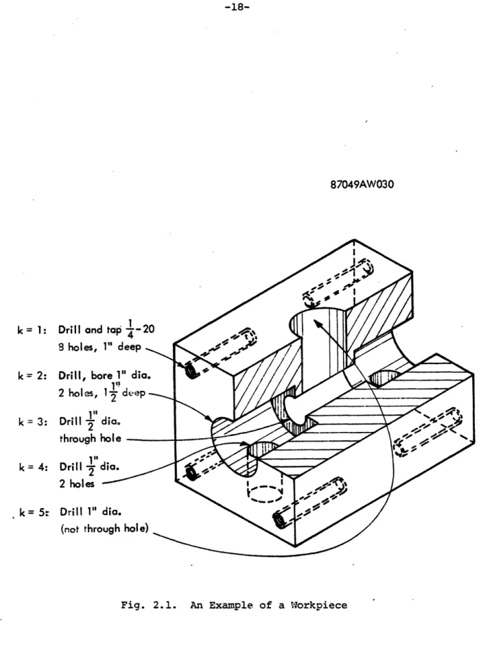
k at workstation j on a piece of type i. The number k represents a particular operation and does not imply that there are strict precedence constraints. As an example, consider the component in Fig. 2.1, which is an idealized representation of the housing for a two way hydraulic control valve. The part is made from a casting which has the correct external dimensions. The operations required are the drilling and tapping of holes to the required tolerances.

A flexible manufacturing system produces a family of such parts which are of different sizes, built to different tolerances and materials. It will be assumed for the sake- of this example that the left hand edge is machined first. The part then goes to the loading station for re-fixturing before the right hand edge is machined. For modelling purposes, the left and right hand edges are identified as two distinct types of pieces each with its own T. matrix.

For the left hand end of the part in Fig. 2.1, the following operations are identified. They are referred to by the superscript k in the variable

k

tij-k=l : Drill and tap the four bolt holes

k=2 : Drill and bore valve chamber to required tolerance k=3 : Drill axial passage

k=4 : Drill and tap outlet lines. k=5 : Drill and tap supply line

The definition of the operations is dependent on the capability of the machines and the distribution of tools amongst them. Operation 2, because of close tolerance requirements,may need a rough cut and then finishing which might not be done at the same machine. Drilling and tapping similarly may

be done at two different machines. In this example, however, we will assume that each operation is completed during a single visit to a workstation.

k= 1: Drill and top 4-20 S holes, 1" deep

k = 2: Drill, bore 1" dia. 0

2 holes, 1' dcep k 3: Drill 2 dia. 2 , through hole - -k= 4: Dri II 2 d:ia 2 holes

1. Operation 2 should precede both operations 3 and 5. 2. Operation 3 should precede operation 4.

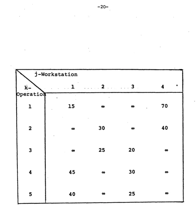
Suppose there are four machines available to manufacture the valve housing. The figures in Table 2.1 show the locations at which the operations can be performed and the length of time in seconds that each operation takes. An entry of - (infinity) indicates that the operation cannot be performed at that location. The top row gives the machine number and the column is the operation number. The element tij of the Matrix Ti will be the number in row k and column j of the table.

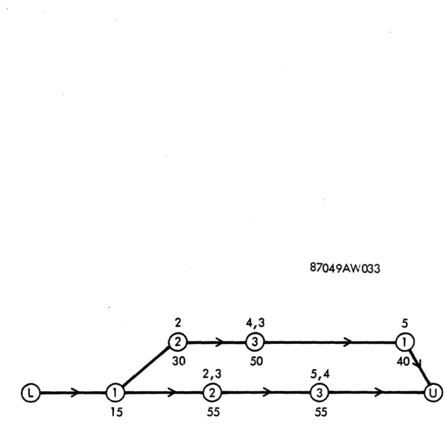
A strategy is a single sequence of workstation visits in which all necessary operations are performed. Two possible strategies are shown in Table 2.2. In strategy 1, operations are performed in the order 1-2-3-5-4, while the order is 1-2-4-5-3 for strategy 2.

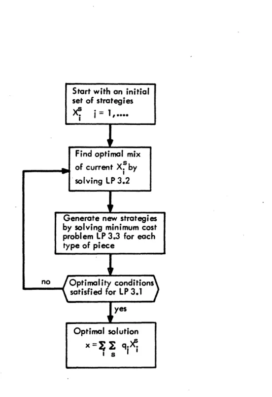
Chapter 3 describes a method of generating strategies during the solu-tion of the optimizasolu-tion problems formulated below.

If the strategies are enumerated in advance, the variable T.. repre-sents the total time a piece following strategy 1 spends at workstation j. In the example above, the variables T..i for strategy 1 are Til = t = 15,

2 3 4 5 1 5 ,

ti2 + t i2 55 andT 4 t + t = 55. Workstation 4 is not

Ti2 i2 i2 i3 i3 i3

used, hence Ti4 = 0. A graphical representation of strategies 1 and 2 of Table 2.2 is shown in Figure 2.2. The number in the circle is the work-station number and the one underneath is the duration of the visit. Above each circle are the particular operations being performed. The initial node L and the final node U are the loading and unloading stations, respectively. Since the operation of the workstations is of primary concern, it will be assumed that the transportation system has a large enough capacity so that it does not reduce the performance of the system. After the important rela-tionships affecting the performance of the workstations are introduced, it will be shown that the transportation system can be easily modelled using the same ideas.

Assuming that the matrices Ti are available for all workpieces, the flow rate1-~ ote pc twk

rate of type i pieces to workstation j for operation k is defined as x.. The

j

-Workstation

.

1

.

2

... 3

4

Operatio

1

15

70

2

co

30

40

=

4

45

=

30

5

40

c

25

c

Table 2.1

.

Machining Times

t

for Operations

1)

at the Workstations

on Part i, the Valve

1

i

1

1

1

2

2

2

2

2

3

3

2

3

3

4

5

3

4

3

5

4

3

5

1

Tab.le 2,2

Two Possible Strategies for the Manufacture

87049AW033

2

4,3

5

30

50

40

2,3

_5,4

15

55

55

system controller monitors these variables and can affect them by varying the loading rate and allocating pieces entering the system to the strategies available.

The total arrival rate X, at workstation j is

P

= I xi j (2.15)

i=l k

k

The variables x.. are related by conservation of flow equations and the production ratio requirement. Conservation of flow states that the flow

rate of pieces undergoing any operation k is equal to the production rate of that type of piece. This is stated as

M k M M

x .. X-l xij = R. i=1,...,P (2.16)

j=l j=1 j=l

where R. is the production rate of type i pieces. The total production rate is given by

P P M

R = R. = x.. (2.17)

i =l i=l j=1

The summation is carried out with k=l for convenience. The production ratio requirement states that pieces of type i comprise a fraction a. of the total production. This can be expressed as a relationship between R in equation

(2.16) and the flow rate of pieces-going for operation number 1

M P M

J-1 1 . ' x

Ie t he s (2.18)

j=1 i=l j=l

where the c. satisfy 1

0 < a. < 1 i=., P (2.19)

ai. = 1 (2.20)

An important performance measure of a workstation is the utilization u., defined as the probability that a workstation is occupied. Suppose that

in an interval of time (0,T) the number of type i pieces passing through

k

workstation j for the operation k is nj.. The total time that the station is occupied is thus

X

nij

i=l k

The utilization can then be written as

Uj T = i- I nij tij (2.22)

i-l k

But it can be recognized that n. i/T is the average flow rate x.. so that

u (X) xij t. (2.23)

ik

The methods of network-of-queues analysis can now be applied so as to

k

express other system performance measures as functions of x=-x...

Optimiza-13 k

tion problems can then be formulated so as to pick the assignments x.. which 13 -maximize the production rate or perhaps some other index of performance.

The total number of customers inside the system either receiving service or waiting in queues is important. Let qj (x) be the average queue length at workstation j. The in-process inventory can then be defined as

M

I = ~ qj(x) (2.24)

j=l

The calculation of qj(x) depends on specific assumptions about the service processes at the workstations. If a manufacturing system has exponentially distributed service times and the arrival of pieces into the network

con-stitutes a Poisson process, the result of Jackson (1963) discussed in Section 2.2.1.can be invoked. The workstations can be studied in isolation as M/M/1 queues. In this case, the average length is (Kleinrock, 1975)

u. (x)

qj(x) = (2.25)

l-u (x)

Similarly if the conditions of Baskett et al., (1975) hold, the relation-ships for M/M/s or M/G/o queues in equilibrium can be substituted in (2.25). For general networks approximate methods can be used to evaluate qj(x).

The presence of pallets in a system causes added complication. From the point of view of the pallets, the system is closed since there are a finite number of pallets circulating in the system. The methods of

analyz-ing closed queueanalyz-ing systems can then be applied. Secco-Suardo (1978) ex-presses the probability distribution function (2.4) for a closed network with N customers as a function of the strategy assignments Yi. He suggests that it is possible to use a non linear programming method to maximize the

throughput of the loading station and thereby attain the maximum production rate. The results of Denning and Buzen (1977) suggest that this method might be applicable to a wider class of systems than that with exponential servers. The optimization problem is one of assigning operations to workstations so as to maximize some performance index. The assignments will be subject to constraints imposed by the problem structure.

In a stochastic system, the two important indicies are the production rate R, which should be maximized, and the in-process inventory I, which should be kept at a minimum. A natural objective function in this case

would be a weighted sum of the two. The weights would reflect the return in maintaining a certain production rate as compared to the cost incurred in

keeping a certain level of in-process inventory. Thus the following non-linear programming problem results:

NLP 2.l M M 1 1

Maximize

X

2x)

(2.26)

-

xl

0

In the objective function (2.26) the production rate of pieces of type 1 is maximized. The ratio constraint (2.28) makes it unnecessary to include the production rate of the other types of pieces. The constraint (2.28) due to the production ratio requirement can be written in a form which is easier to evaluate since it does not involve summing over all the types of pieces.

M a, M

I X.ij a . 1Xlj 0 (2.31)

j=l i3 a1 j=l

Equation (2.27) is the flow conservation constraint. The limited capacity of the workstations results in (2.29) which states that the utilization of any workstation can not exceed unity if a steady-state equilibrium is to be reached.

It should be noted that it is not necessary to identify strategies in order to formulate NLP2.1. This point will be discussed in Section 2.3 and further elaborated on in Chapter 3.

The problem NLP2.1 can be modified. There might be cases where the average in-process inventory is required to remain below a certain level Q. This can then be expressed as a constraint to give NLP2.2

NLP2.2 M Maximize ' xij (2.32) j=l 1] subject to (2.27), (2.29), (2.30), (2.31) M and I q.(x) < Q (2.33) j=1

Where queue lengths grow without bound as utilization approaches unity, constraint (2.33) may make (2.29) redundant.

Enumerating Strategies in Advance

There are instances where it is either necessary to enumerate strategies in advance or the number of possible strategies is not large and they can be readily identified. For example, if the four workstations in the example given above are arranged linearly, as in Fig. 2.3, there are then only two possible strategies. They are depicted in Fig. 2.4. The number of possible

strategies Si for a given piece normally depends on the nature and number of the operations and not just the geographic layout of the workstations.

Let yt be the flow rate into the network of pieces following strategy Q. The production rate is the total flow rate into the network r

S

Z

':

4

§

where

p

S =

7

The arrival rate X. at workstation j is

X. = Y (2.35)

sm(j)

where m(j) is the set of strategies that use workstation j. The utilization is given by

Uj = j (2.36)

kem(j)

These quantities can be used in NLP 2.3 and NLP 2.4 to find the optimal mixture of strategies in the system. The two programs NLP 2.3 and NLP 2.4 are analogous to NLP 2.1 and NLP 2.2 respectively. The relationship be-tween yR and xij is given by equation (2.43) and (2.90).

NLP 2.3 S M Maximize 1

7

7i

NLP 2.4 Maximize I y (2.41) 4=1 subject to (2.38), (2.39), (2.40) and M I ((y) < 0 (2.42)

j=l

Constraint (2.39) expresses the production ratio requirement. In calculating the average queue length q4(y) at the workstations, use is made of (2.35) which expresses the arrival rate at a workstation as a function of strategy assignments y

Modelling of the Transportation System

The transportation system can be modelled as a network of arcs and nodes. The nodes are either merges or diverges of arcs, or the actual workstations themselves. It is natural to view most transportation systems as trans-portation networks (Magnanti, 1977). Hence network models are applied to a wide class of transportation systems. In flexible manufacturing systems, network models can be used to model conveyer belts or systems where pieces

are carried on a vehicle moving along a guideway.

For convenience, it is assumed that the nodes are numbered so that the first M are workstations and the remainder merges or diverges. Further-more it is assumed that the arcs are numbered so that arc i leads to

worksta-tion i, with the rest of the arcs being numbered M+l, M+2, and so on. The arc leading into the loading station is labelled 0. This allows congestion effects at the loading station to be modelled. The network of Fig. 2.3, for example, has the labels shown in Fig. 2.4. The circled numbers re-present nodes while the rest are arc numbers. Define r.. as the flow rate

13

of type i pieces on arc j of the network. From the definitions,

r..i = x. j = 1,....,M (2.43)

The problem NLP 2.1 can be modified to become NLP 2.1a P M Maximize ri - x) (2 + gqr) (2.44) i=l j=1 subject to (2.27), (2.29), (2.30), (2.31), (2.43) and I r.. - Y r.. = 0 V n (2.45) jEA(n) 3 jD (n) ir.. < d (2.46) r.. > 0 (2.47)

where the rio is the flowrate of type i pieces into the network. The con-straint (2.45) expresses flow conservation at network nodes in which A(n) is the set of arcs leading to node n and D(n) is the set of arcs carrying pieces away from the node. Arc capacity constraints if present are expressed by (2.46)

The in-process inventory consists of pieces queueing at the workstations qi(x) and those in transit in the network g(r). The derivation of g(r) is dealt with below. The total in-process inventory is thus on average

M

I = I qj( x) + g(r) (2.48)

j=l

This is incorporated in the cost function (2.44). Similarly NLP 2.2 can be written as

NLP 2.2a

Maximize

7

and

%(X)

+

<

xik rij > ° (2.50)

The number of pieces on any arc l in the network is on the average given by

·Z = ft t. (2.51)

where fZ is the total flow rate on the arc and tZ is the average travel time on the arc. This is an example of Little's formula (Kleinrock, 1975). If the arcs are subject to congestion effects, the travel time is then an increasing function of the total flowrate fZ. The total flow rate is given

by

fz= ri _(2.52)

Then g(r) = I (2.53)

Z>M Z

The transportation system can be handled in a similar fashion where the strategies are enumerated in advance.

The transportation network has path constraints characterized by net-works of possible strategies such as Fig. 2.2. Each arc on the strategy network corresponds to a flow between two workstations. In a densely

connected transportation system, there is a choice of paths between the two workstations while a simple system as in Fig. 2.5 provides no choice.

Chapter 3 has a further discussion of these constraints and how the net-work structure may be exploited in order to solve the routing problem. 2.3.2 Modelling of Deterministic Systems

A deterministic flexible manufacturing system is one in which the processing times are entirely deterministic. The arrival process into the

0

L

Z

O

30

~

oCC.

system is deterministic in the sense that workpieces can be introduced into the system at pre-determined time instants. The assignment problem can be formulated and solved as a job-shop scheduling problem (Fisher, 1970). There are added complications however. An optimal steady state assignment is being sought. This means that the number of jobs to be assigned is not only undetermined, but it is also likely to be large. For a similar reason, the time interval over which the assignments have to be made is undetermined. Each of the jobs to be scheduled has options as to which workstation it can go to for a particular operation. All of these factors increase the size and complexity of the scheduling problem. From a control point of view, precise schedules worked out in advance are difficult to implement, especial-ly over long time intervals.

One way of overcoming these difficulties is to use a periodic schedule (Hitz, 1979). A periodic schedule is one in which a certain sequence of operations at the workstations is repeated at regular time intervals. There is a set of integer numbers ni, i=l,...,P such that

p

n. = .i nz (2.54)

if ni is the number of type i pieces to be manufactured in a period. A schedule is sought in which there is no idle time on the bottleneck work-station. The bottleneck is the station j that maximizes i..jni, in which

i1

Sij is the total time that pieces of type i spend at workstation j during their manufacturing process. The schedule should be such that it can be repeated without leaving any idle time on the bottleneck workstations. In order to derive iij' the strategies used to manufacture each of the pieces should be determined; then Eij = E TZj.

The aggregated flow approach used in stochastic models affords a way of simplifying the assignment problem. It will now be extended to deter-ministic systems.

k

Consider a time interval (0,T). Let n.. be the number of type i pieces 1)

that are sent to workstation j for operation k in the interval (0,T). The k

assignments n.. are to be made in a manner which maximizes the total pro-duction while maintaining the ratio requirement (2.54). The following integer program can thus be solved in order to achieve this objective:

IP 2.1 M- P Maximize

y

The objective function (2.55) is the total production. Constraint (2.56) requires that all operations are carried out on all the pieces. Expres-sion (2.57) reflects the fact that all manufacturing processes must be completed in the inverval (0,T). The solution of IP 2.1 could serve as a basis for the periodic scheduling algorithm. The problem would be in determining T, which would then be the period of the schedule.

The flow rates in the interval (0,T) can be defined as k

k n. .

x.. =

-

-

T

With this transformation, consider the following linear program derived from IP 2.1

LP 2.1

Maximize X xij (2.60)

i j

M 1 P M

s.t. Y.; X..I .1 X..I (2.61)

j=l 1) 1 i=l j=l

I X1 i ,j X (2.62)

I _i I _k x. t < _kk1 (2.63)

ik

kX 0 (2.64)

The relationship between LP 2.1 and NLP 2.1 or NLP 2.2 is obvious. The constraints (2.61), (2.62), and (2.63) are identical to (2.28), (2.27), and (2.29) of NLP 2.1 or NLP 2.2. The deterministic problem does not

take into account the buildup of queues within the system. This ac-counts for the difference between LP 2.1 and the non-linear programs in

the stochastic case.

If xj.. is the optimal solution of LP 2.1 then

fi..

IP 2.1 if Tx.. is integer. Otherwise it provides an upper bound on the optimal

1)

value of the production rate. The time horizon over which the optimal assign-ment is carried out is long compared to the operation times t... Thus the

Ak

numbers n.. are large. The difference between the optimal solution of IP 2.1 and n.. are thus negligible (Salkin, 1975).

Secco-Suardo (1978) derives a similar linear program for maximizing the throughput of a network modelled as a closed network of queues. In the limit as the number of customers inside the network grows large, it is found that the throughput is proportional to the ratio of the relative utilization of the bottleneck workstation to that of the loading station. The problem is then one of finding the max min u. (x). This is formulated

as a linear programming problem similar to LP 2.1.

Baskett et al.., (1975) show that the marginal probability distribution of having n customers at a queue depends only on the mean serVice and arrival rate. This indicates that the asymptotic result holds for general networks

satisfying Baskett et al.'s (1975) assumptions. Furthermore, as a variance of the service time distribution goes to zero, the linear program described is unchanged as long as the assumptions - including that service time dis-tributions have rational Laplace transforms - remain satisfied. The

deterministic case can thus be viewed as a limit of the class of systems to which the stochastic network of queues theory applies.

The work rate theorems of Chang and Lavenberg (1972) show that the throughput of a closed network is proportional to the ratio of the relative utilization of the bottleneck station and the loading station. They make no assumptions regarding the queue discipline. The only restriction on service time distributions is that they should have finite non-zero expectations.

The linear programs of this chapter yield the maximum asymptotic throughput solution for networks with general service time distributions. It should be noted however that they do not take into account the build up of queues within the network.

2.4 An Approximate Method for Finding the Production Rate of a Balanced Closed System

The linear programming formulation of Section 2.3.2 finds the limit-ing maximum production rate in a closed system as the number N of pieces

in the system becomes large. The effect of a limited number of pallets is important. Simulation results show that the production rate of the system increases asymptotically to a maximum value as the number of pallets inside the system increases (Horev et al., 1978). Closed queueing network models also exhibit this rise in throughput as the number of pieces inside the network grows (Ward, 1980) (Secco-Suardo, 1978).

An estimate of the production rate as a function of the number of pallets can be derived. In a system where there are only single server

that there are ni pieces at station i is given by (Gordon and Newell, 1967) M n. 1 1 P(nl' n2'..nM) = (MN) Xi (2.65) with M = number of stations N = number of pallets

X. = relative utilization of station i

and

in.= N (2.66)

The relative utilization is defined as

e.

X. = (2.67)

where pi is the service rate of station i, and ei are constants satisfying

e. = Pie. with Pji being the probability that a workpiece goes to

. j=l 31ji 31

station i immediately upon completion of service at station j. The factor G(M,N) is a normalizing constant,

M n.

G(M,N) = I I X (2.68)

1 S i=l

where S is the set of all partitions of N pieces at M stations.

Assume that the system is balanced in the sense that all stations have the same relative utilization. Then,

e.

X. = = X Vi (2.69)

Substituting (2.69) into (2.68) gives M n.

G(M,N) =

x

S S

The number of partitions in S is M( 1 The normalizing constant is then

(MN) N+M-1 XN (N+M-1)! N(271)

G(M,N) = M (2.71)

IM-1) (M-l)!N!

The throughput T. of station i is given by (Secco-Suardo, 1978)

G(M,N-1)

Ti = ei G(MN) (2.72)

From (2.71) and (2.69) this can be written as

T. - N (2.73)

i N+M-:1 i

The assumption behind (2.73) is that the utilizations of all stations in a balanced system are equal for all values of N. If R is the limiting maximum production rate of the balanced system, the actual production rate if the number of pallets is limited is

P = R (2.74)

N+M-1

This is established by noting that P is the throughput of the loading station. The relationship (2.74) then follows naturally from (2.73).

The approximation can be extended. If in (2.65) there are (M-l) balanced stations and station M (for convenience) has a relative utilization

M-1 n. nM

G(M,N) = I (X 1) (qX) (2.75)

S i=l

This becomes

G(M,N) = XN E qM (2.76)

This model corresponds to the practice of modelling the loading station and transportation system as a server in a closed network of queues model.

Its utilization is usually lower than that of the servers corresponding to the workstations.

Equation (2.76) is a polynomial in q with nM = 0,...N. The coefficient

N

of q is X times-the number of partitions of (N-nM) pieces in (M-l) machines and is given by N+M-2-\ ). Thus

M-2

G(M,N) = XN i (N+(M-2)-i) (2.77)

i=0 (N-i) I (M-2)

The expression G(M,N-1)/G(M,N) is thus a ratio of two polynomials N-l X biqi G(M,N-1) i=0 (2.78) (2.78) G(M,N) N X

Y

ai+l N-i

= _______ (2.81)

a. N+M-2-i

Thus if M > 2, then a < a.. i+l 21

The probability that there are nM = j pieces at the nonbottleneck station is,from (2.65) and (2.75)

N

PM( j) = G(M,N) a q (2.82)

Since q is less than 1 and ai+l < a. for M > 2, then PM(j+l)< PM(j). If q is sufficiently small, or in other words if the nonbottleneck station is much faster than the other balanced stations, it is reasonable to ap-proximate G(M,N-1)/G(M,N) by considering only the coefficients ao and alof the polynomials. This gives an approximation with the form

G(M,N-l) 1 1 (2.83)

G(M,N) X A+Bq

where A and B are constants. By equating coefficients for the first two terms in (2.78) and applying (2.80),

A =N+-2 (2.84)

N

B = (2.85)

N(N+M-3)

Substituting into (2.83) gives the expression

G (M,N-1) 1 N (N+M-3) (2.86)

Note that for q = 0,

G(M,N-1) 1 N G(M,N) X N+M-2

This is equivalent to (2.74) but with one station less. In practice, the expression (2.86) is found to vary only slightly with q (Fig. 2.6) and it is better to use the simple expression (2.87) since it involves less com-putation.

To generalize, if the number of bottleneck stations, MB, with equally

high relative utilization is larger than two, an approximation to the production rate P as a function of the number of pallets and the limiting maximum production rate, R, is

N

P =N+ R (2.88)

N+MB1

The equation (2.88) is useful because for a balanced system it is possible to obtain a good assessment of the production rate and the number of pallets required by solving a linear program and a simple equation. It is also possible to estimate the return from an investment on pallets. In a system with four balanced workstations, it takes approximately 27 pallets to have a production rate 90% (i.e., XG(M,N-.) = 0.9) of the limiting rate.

G(M,N)

To raise that to 95% requires an additional 30 pallets. This assumes

stochastic effects which are implicit in the closed queueing network model. The rate at which the ratio XG(M,N-1)/G(M,N) approaches unity as N +X is important. It determines the number of pallets that are needed in a system in order to have a production rate close to the asymptotic maximum. The rate depends on the number of bottleneck stations in the system. The more balanced the system is, the slower the convergence. Intuitively this may be explained by the fact that in a balanced system, the pallets

distribute themselves evenly at the machines. The asymptotic production rate is achieved when there is no idle time at the bottleneck stations.

cv,

o

o

~o

t

o

Thus the more balanced a system is, the larger the number of pallets needed to do this. In Fig. 2.6, the ratio (2.87) is plotted for two different values of M and it can be seen that for the higher value of M, it approaches

the asymptote much more slowly than for the lower value.

It may happen that the highest asymptotic production rate is achieved by a strategy assignment which produces a balanced system. It is also possible that for finite N, a different assignment leading to an unblanced

system has a higher production rate. This is because the unbalanced system approaches its limiting production rate faster than the balanced system as N increases.

In Fig. 4.19, the throughput as a function of N for a four-workstation system modelled as a closed network of queues is shown. For N=13, the production rate for the unbalanced system is the same as that of the bal-anced system. The balbal-anced system needs about 30 pallets to reach 90% of its asymptotic throughput whereas the unbalanced system needs only 15. As N increases, the balanced system has a higher throughput.

In choosing the optimal mix of strategies, the number of pallets, if small, should be considered. The optimization model suggested by Secco-Suardo (1978) is a method of tackling such problems.

2.5 Some Characteristics of the Solutions of the Optimization Problems Let x.j denote an optimal assignment of operations in a flexible

13

manufacturing system. The constraints due to the workstation capacity limitation are, at the optimal point

Xi

i

n P 2.1 some will be satisfied as equality constraints and the others ask

In LP 2.1 some will be satisfied as equality constraints and the others as inequalities. The workstations corresponding to constraints satisfied as equalities are the bottleneck stations. The production rate of the system can only be increased for a particular parts requirement by increasing the speed of the-bottleneck workstation (i.e., decreasing tk. for bottleneck stations).