Evaluating Multi-User Selection for Exploring Graph Topology on Wall-Displays

HAL Id: hal-01348578

https://hal.archives-ouvertes.fr/hal-01348578

Submitted on 25 Jul 2016

HAL is a multi-disciplinary open access

archive for the deposit and dissemination of

sci-entific research documents, whether they are

pub-lished or not. The documents may come from

teaching and research institutions in France or

abroad, or from public or private research centers.

L’archive ouverte pluridisciplinaire HAL, est

destinée au dépôt et à la diffusion de documents

scientifiques de niveau recherche, publiés ou non,

émanant des établissements d’enseignement et de

recherche français ou étrangers, des laboratoires

publics ou privés.

Evaluating Multi-User Selection for Exploring Graph

Topology on Wall-Displays

Arnaud Prouzeau, Anastasia Bezerianos, Olivier Chapuis

To cite this version:

Arnaud Prouzeau, Anastasia Bezerianos, Olivier Chapuis.

Evaluating Multi-User Selection for

Exploring Graph Topology on Wall-Displays.

IEEE Transactions on Visualization and

Com-puter Graphics, Institute of Electrical and Electronics Engineers, 2017, 23 (8), pp.1936–1951.

�10.1109/TVCG.2016.2592906�. �hal-01348578�

Evaluating Multi-User Selection for Exploring

Graph Topology on Wall-Displays

Arnaud Prouzeau, Anastasia Bezerianos, Olivier Chapuis

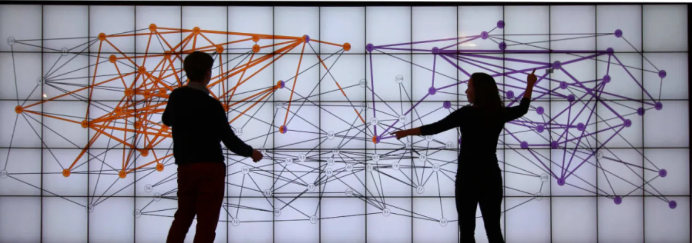
Figure 1. A pair using the propagation technique to explore a graph. They discuss two communities, in orange and purple, selected using the propagation technique. The communities are linked by a specific node shown by the right user. The remaining 3 orange-purple nodes show how by propagating the purple community, it flows into the orange one through this node.

Abstract—Wall-displays allow multiple users to simultaneously view and analyze large amounts of information, such as the

increasingly complex graphs present in domains like biology or social network analysis. We focus on how pairs explore graphs on a touch enabled wall-display using two techniques, both adapted for collaboration: a basic localized selection, and a propagation selection technique that uses the idea of diffusion/transmission from an origin node. We assess in a controlled experiment the impact of selection technique on a shortest path identification task. Pairs consistently divided space even if the task is not spatially divisible, and for the basic selection technique that has a localized visual effect, it led to parallel work that negatively impacted accuracy. The large visual footprint of the propagation technique led to close coordination, improving speed and accuracy for complex graphs only. We then observed the use of propagation on additional graph topology tasks, confirming pair strategies on spatial division and coordination.

Index Terms—Wall-Displays; Multi-user interaction; Graph visualization; Selection techniques; Co-located Collaboration

F

1

I

Graph structures, consisting of vertices and edges, exist in vari-ous application areas: in social networks they are used to represent people and their relationships, in molecular biology proteins and their interactions, in transport networks they can represent air-flight routes, etc. Graph data structures are frequently represented as node-link diagrams, but like many visual representations of large datasets today, they can be too wide to view comfortably on regular screen monitors [64].

High-resolution wall-sized displays [8, 54] are promising data analysis environments, as their size and high pixel density allow simultaneous viewing, comparison, and exploration of large amounts of data. Their size can also comfortably accommodate multiple viewers, supporting collaborative analysis [60]. Despite their promise as collaboration platforms, they have received little attention for graph exploration. We take a step in this direction. • Arnaud Prouzeau is with Univ Paris-Sud & CNRS (LRI), Inria, and

Universit´e Paris-Saclay. E-mail: arnaud.prouzeau@lri.fr

• Anastasia Bezerianos is with Univ Paris-Sud & CNRS (LRI), Inria, and Universit´e Paris-Saclay. E-mail: anab@lri.fr

• Olivier Chapuis is with Univ Paris-Sud & CNRS (LRI), with Inria, and Universit´e Paris-Saclay. E-mail: chapuis@lri.fr

We present a systematic study of how pairs use a wall-display to solve topology based tasks, that are common components of more complex graph analysis tasks [37]. We study how the choice of interaction technique supports or hinders pairs collaborating on these tasks. We focus on techniques for selection, a fundamental visualization task, as it is a pre-requisite to many interactions such as filtering, comparisons, details on demand, etc.

We adapt two general purpose graph selection techniques for use by multiple users on a touch-enabled wall-display. Our baseline is an extension of basic node/edge selection for multiple users. It is easy to master, and has a limited, and thus fairly localized, visual footprint on the wall display, that does not inter-fere with colleagues’ work. The propagated selection extends for multiple users the idea of transmitting a selection to neighboring nodes/edges [21,42]. It highlights the connectivity structure of the graph (Figure 1), but may have a large visual footprint that disturbs colleagues.

We first assess the impact of selection technique on pairs conducting a specific topology analysis task, namely identifying a shortest path. As there is no work on pairs working on such tasks on wall-displays, we tease out effects due to the technique or due to collaboration, by also studying single user selections. We

This is the authors’ accepted version of the article (sent 4 March 2016; revised 17 June 2016; accepted 14 July 2016). The definitive version will appear

then examine how propagation, the most promising technique, is used by pairs on other graph analysis tasks [37]. Our studies are conducted on a touch enabled wall-display, instead of interacting using mice and keyboards, as mobility allows viewers to perform implicit zooming [7] and correct for visual distortions [10].

We contribute: (i) The adaptation of two graph selection techniques for collaboration on wall-displays. (ii) The controlled study of how pairs use these techniques on a graph topology task (shortest path identification) on wall-displays. (iii) A discus-sion and observational study on how one technique, propagation, supports different topology tasks. And (iii) a set of design impli-cations: as pairs divide the work spatially, even when tasks are not spatially divisible, the use of a localized selection technique may be detrimental to performance in complex graphs; while a technique with global reach leads to tighter collaboration and coordination, that is more effective and accurate for such graphs.

2

R

W

A wide range of topics surrounding large displays have been studied in HCI and Visualization. We focus on the most relevant, namely visual exploration and collaboration on wall-displays, in particular exploration of graphs, and the idea of transmission. 2.1 Walls in Visual Exploration

Wall-sized displays have been studied in the context of infor-mation visualization and analysis, as they can naturally display a large amount of visual information. Previous work comparing large displays to traditional desktops [40,58] or to smaller displays [52] has shown performance improvements when moving to larger displays. Considering visual analysis in particular, Yost and North [68] tested several data visualizations for their scalability when moving from small to large displays. They found their visualiza-tions to scale well for the tasks of finding detailed and overview information, and note that spatial encoding of information was particularly important on large displays. Jakobsen and Hornbæk [31] examined the interplay between display size, information space size and scaling, and found that all these factors need to be taken into account, and that increased display size did not improve navigation performance in tasks where targets are visible at all scales. Reda et al. [52] found that larger displays encourage longer visual analysis sessions, and result in deeper and more complex insights. Finally, Rajabiyazdi et al. [51] observed that they can lead to previously missed insights in multiple disciplines.

Beyond their benefits, researchers have studied specific issues related to visual perception of wall-displays due to their scale. En-dert et al. [17] discuss how a viewer’s distance from the wall influ-ences the visual aggregation of displayed information. Bezerianos et al. [10] showed large discrepancies in the perception of basic visual encodings depending on viewing distances and angles, that nevertheless decrease if appropriate physical navigation is used. Ball et al. [6] compared the benefits of added peripheral vision vs. physical navigation, and found that physical navigation influenced task performance while peripheral vision did not. Isenberg et al. [28] blended two visualizations so that each is perceived at a different viewing distance from the wall. Collectively this work stresses the importance of physical navigation for visualization and visual perception tasks, even if it is not necessarily better than virtual navigation in classification tasks [33].

Despite the importance of physical navigation, a large body of this past work either assumes the use of mouse and keyboard,

or simply does not study interaction. Nevertheless, recent work supports both interaction and physical navigation using handheld devices or direct touch. Handhelds are used as touch-pads to conduct classification tasks [40], or as a support for physical con-trollers [34] or for explicitly sketching interactive slider controllers [61] to conduct multi-dimensional data exploration. In a sense-making task, Jakobsen and Hornbæk [32] allow users to move freely and use direct touch to interact with the wall. We similarly use touch to support pairs working on graph topology tasks. 2.2 Walls in Collaborative Analysis

When it comes to co-located collaborative work and visual anal-ysis (see [22, 29] for reviews), work has focused mostly on tabletops, and “small” vertical displays (SDG and whiteboards). For example, researchers have explored how collaborators shift from tight to loose work coupling [59], how users divide space (territoriality) [62], how they analyze text documents [30], com-pare tree visualizations [26], etc.

There are few works on co-located collaborative work on large (ultra-high resolution) walls. Notable exceptions are recent work by Jakobsen and Hornbæk [32] that studies the behavior of a pair of users in a sense-making task, and Liu C. et al. [39] that studies the effect of different collaboration styles and interaction in a classification task. Both these works stress the importance of users’ coordination (possibly at distance) in these environments. Our work is along the same lines, but focuses on graph analysis in particular, and the effect of different interaction techniques on it, a topic that so far has not been studied.

2.3 Graph Exploration on Large Surfaces

Collaborative analysis is one of the next challenges of the analysis of graphs [64]. Existing systems support mainly remote collab-oration (e.g. [69]). Less work has targeted co-located analysis, like that by Isenberg et al. [27] that retrofitted an existing graph visualization application for use by multiple analysts with mice and keyboards. We are not aware of any work that studies analysis of graphs by multiple users moving freely in front of wall-displays. Although work on graph exploration using wall-displays is limited, researchers have identified their potential early on. For example, Abello et al. [1] used a wall display to visualize communication network data. Later, Mueller et al. [47] designed an algorithm to interactively layout graphs optimized for tiled displays and distributed environments, while Marner et al. [41] let users interactively adapt the layout on the wall using a mouse and keyboard. Finally, Lehmann et al. [38] leverage physical navigation as an implicit interaction, using the viewer’s distance from the wall to adjusted the level of detail of a graph, and Kister et al. [36] use it to move a lens with contextual information. This past work on wall displays does not study the use of explicit interactions (e.g., selections) during collaboration, as we do.

Finally, although not explicitly testing collaboration, re-searchers have introduced multi-touch techniques for manipulating graphs on interactive tabletops. For example, Henry Riche et al. [23] use multi-touch interactions to fan out links leaving a node, to bundle them, or use link magnets to attract certain types of links. Schmidt et al. [55] alter link trajectories, pin, or make them vibrate by plucking them. This work introduces multi-touch techniques on tabletops for different purposes. While we also use touch, we focus specifically on selection and study how pairs use it to perform graph topology tasks on wall-displays.

2.4 Graph Exploration using Transmission

Visual analysis of graphs is a long standing field, with numerous research questions (see [24,64] for reviews). We focus on tech-niques related to our propagation selection (section3.2), that use the idea of propagating/transmitting information to neighboring nodes or links that is central to graph analysis (e.g., [53]).

As graph structures can be very large, exploration is often localized on interesting nodes and their neighbors. For example, van Ham and Perer [63] designed a Degree-of-Interest function for graph exploration that first proposes interesting nodes, and lets the user indicate interesting nodes to expand to. Archambault et al. [4] use specifically the notion of distance to progressively reveal and render nodes proximal to a node of interest from within a larger graph hierarchy. Moscovich et al. [46] propose interaction tech-niques for panning within a graph, or bringing neighbors closer, based on the graph’s connectivity. Finally, egocentric techniques (e.g., [67]) re-layout graphs by focusing around one node and laying out the rest based on their distance from it; or focus on two nodes [13] and highlight their common neighbors. This work can lead to a user-driven re-layout of the graph, that may disrupt the work of other viewers in a multi-user setting.

Other techniques related to propagation preserve the layout. Heer et al. [21,20], allow users to highlight the contour of the 1st or 2nd degree neighbors, or the connected component of a node, by hovering over it or by using repeated mouse clicks. McGuffin and Jurisica [42] propose techniques to locally select and manipulate nodes, including a menu option that selects a node’s neighbors of increasing distance progressively. Ware and Bobrow [65] evaluate different means of highlighting connections to neighbors of arbitrary degree specified by a text field, and found that motion representations are not better than static highlighting. We extend this notion of propagated selection to multiple origin nodes, providing appropriate input and visual design, to support such selections by multiple users.

3

I

T

Our goal is to investigate how interaction techniques affect mul-tiple users working on graphs. We focus on selection, as it is a required first step for many other visualization tasks, such as filtering, comparison, details on demand, etc. Two techniques were considered, a simple selection (Basic), and one based on the graph’s connectivity structure (Propagation). These techniques were chosen due to their properties: they can benefit graph explo-ration differently but also face different challenges when adapted for multiple users on wall-displays. We describe next how we adapted the techniques for touch interaction on wall-displays, and for collaborative use. Each description finishes with a summary of the technique’s properties, motivation for their use, and possible challenges when used in a multi-user context on wall displays. 3.1 Basic Selection

Basic is inspired by colored selections available in graph visu-alization software extended for multiple users. We chose it to investigate the limits of basic selections in collaborative settings. 3.1.1 Interaction and Visual Design

A node (or link) is selected by tapping on it once, and deselected if tapped again. Inspired by previous work [4, 21], we also highlight the links (or nodes) attached to it so as to demonstrate its connections, but do not re-layout the graph to avoid disrupting

collaborators. Given that we do not have keyboard modifiers, and wanted to keep the touch input vocabulary simple, we decided to allow users to modify this selection in the following way: if the user taps on a node adjacent to an existing selection (direct neighbor), then this node is added to the selection and it, and its links, are highlighted with the selection’s color. If the node is adjacent to more than one existing selections it takes the color of the last edited selection. Tapping on a selected node removes it from the selection. This way users can edit their selections with simple taps, keeping the input vocabulary very simple. We chose to not use lasso-type selections that require dragging to select multiple items, as they are not well suited to large interactive surfaces, such as walls, where prolonged dragging is inaccurate, fatiguing [25], and often disrupted by bezels in tiled walls.

Our wall, similar to many touch enabled surfaces, does not differentiate between users. Nevertheless, it is important for col-leagues to differentiate their work. Thus, if users tap on nodes that are not adjacent to existing selections, we assume a new selection is being made (potentially by a different user) and assign it a new color, chosen randomly from a set that is easily distinguishable. 3.1.2 Summary

Basicextends the simple selection available in graph visualization software to selection of multiple nodes/edges by multiple users. It is familiar, easy to understand, and our design ensures it relies on simple taps. It has a small visual footprint as it selects a single node and its edges at a time, and thus will likely not disrupt collaborators when used in a multi-user context on wall displays. Nevertheless, it may require extensive physical movement if users need to select multiple nodes that are far away on the wall. 3.2 Propagation Selection

As an alternative, we investigate Propagation selection, based on the idea of progressive transmission of a selection to neighboring nodes. Propagation allows local interaction on a node that can highlight its influence across a larger area on the graph (and wall), without requiring extensive physical movement that can be tiring. Nevertheless, it may have a large visual footprint if neighboring nodes are far away, potentially disrupting collaboration.

Variations of the propagation selection from past work (e.g. [21,42]) allow a single user to either highlight neighboring nodes up-to a specific degree only [21], usually 2, or use a menu or text option to select a node and its neighbors of a certain degree [42]. We explain how we adapted the technique allowing multiple users to easily expand the selection to the n-th degree using simple touch interactions. We finally describe its properties and how it can be used to perform topology-based tasks [37] when analyzing graphs. 3.2.1 Interaction

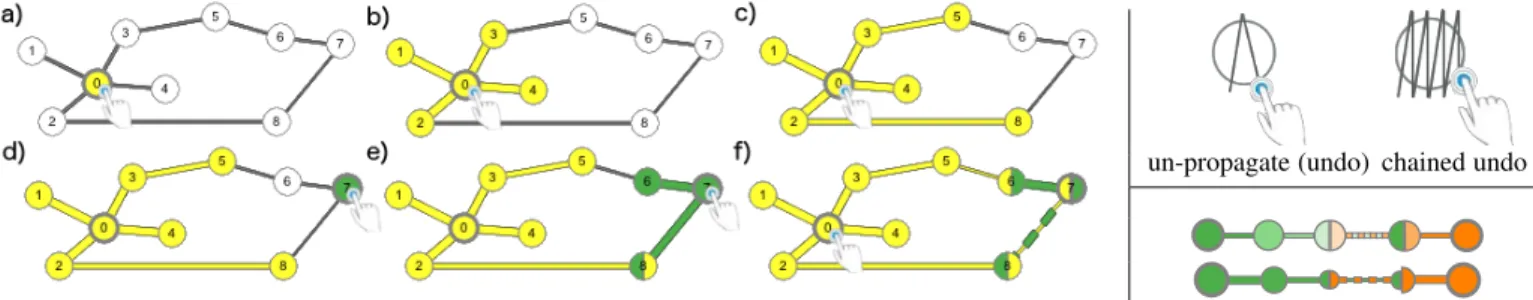
Propagation allows users to select a node, which we will refer to as the origin, and then propagate the selection first to its neighbors, then to their neighbors, and so on. Propagation of a selection is done through a series of taps (clicks) on a node. The first tap selects the node itself (Figure 2-a), and the following taps propagate the selection progressively to the neighboring edges and nodes: the second tap adds to the selection outgoing links and first-degree neighbors of the origin (Figure 2-b), and so on for all following taps1 (Figure 2-c). If users continue tapping,

1 _{Propagation starts either from a node or a link. To simplify the discussion we} talk about node propagation, but we use a similar selection pattern for links: link selected first, adjacent nodes and their links next, and so on.

un-propagate (undo) chained undo

Figure 2. On the left multiple propagations: (a) a first tap on node 0 selects it; (b) a second tap propagates the selection to immediate neighbors; (c) and a third tap to 2nd degree neighbors (notice the difference in link width according to distance); (d) a tap on node 7 selects it with a new color; (e) a second tap selects its neighbors, one of which (node 8) is shared with the first propagation and has both colors; (f) a fourth tap on node 0 propagates the first selection a third time, resulting in nodes 6,7,8, and link 8-7 being shared between propagations, with the color and width on shared link 8-7 alternating. On the top right gesture to undo one propagation step on a node (left) and chained undo for backtracking multiple steps (right). On the bottom right design variations for displaying propagation distance using color intensity (top) and node-link size (bottom).

propagation continues until no more nodes can be reached from (are connected to) the origin node. Thus a propagated selection is a progressive query selection, that adds elements connected to the origin node at progressively increasing distances.

We note that the first step of propagation (selecting only the node) is not the same as Basic (selecting the node and its edges). We made this design choice as initial feedback indicated that the metaphor of transmission is better served if we consider that each tap opens the flow of transmission from the selected nodes to their neighborhood (both links and nodes).

To accommodate multiple users working in parallel, when users select a node that is not part of an existing propagated query, it becomes the origin of a new propagation selection (Figure 2-d). If they select a node already inside a propagation query (but not its origin), the query expands to also include propagations from this new origin. Thus one propagation query can have multiple origins. As we designed the technique for touch surfaces, we chose a simple crossing zig-zag gesture to undo propagation steps. When performed on the origin, it backtracks the propagation by one step (Figure 2left). The gesture can be chained to perform multiple backtracks without lifting a finger, undoing quickly several prop-agation steps in one interaction. When the selection is reduced to a single node (the origin), this gesture unselects the node.

A crossing gesture on an element (node or link) that is not the origin of a propagation, removes this node from the selection and blocks future propagation paths of this selection to go through it. 3.2.2 Visual design

Nodes and links in a propagated selection share a common color (as traditional color queries). Propagation origins stand out with a thicker border (Figure 2-a), and new propagations are assigned a different color, similar to Basic (Figure 2-d).

Due to the propagation of selections, a node can be selected by two or more colors. The node in question is divided visually into slices equal to the number of selections, and given the respective colors (Figure 2-e).

Links can similarly be part of several selections. Dividing them in segments equal to the number of selection colors (similar to nodes) could lead to few, but long, colored segments if links are long. Thus the multiple colors could be hard to see locally on a wall display. We decided instead to streak (dashing pattern) the links with the selection colors (Figure 2-f). We fixed the number of streaks to seven, as we observed that on our wall they were still visible locally, even on long links. Moreover, as the fixed number of streaks have different length depending on the total length of the link, they give locally an indication of its overall length.

We explored different design variations to emphasize the distance of elements (nodes and links) from the origin. This is of interest both within a single selection (to identify the farthest elements), but also for elements that are part of multiple selections to identify which origin is closest. As color is already used in selections, we considered other visual variables (Figure 2 right). Color intensity that drops with distance was considered, but rejected, as the perception of intensity may be affected by viewing distance and angle across the wall-display, and color intensity may vary across screens in tiled wall-displays [57]. We thus chose the size of elements, i.e., the thickness for the links and the radius for the node slices. While testing our prototype, we observed that as nodes have multiple incoming links, it is hard to identify which path and origin is responsible for the shortest distance that determines their size. Thus to avoid confusion and reduce clutter, we chose to only display distance information on the links.

As the thickness of selected links indicates their distance to the propagation origin node, the thicker the link the closer to the origin it is. We chose to display three visual levels of thickness: links with maximum thickness are linked to first-degree neighbors, ones of medium thickness link first and second-degree neighbors, and all remaining links selected through propagation have a similar minimum thickness. We found that more levels led to small variations in thickness that were hard to perceive in dense graphs. When a link is traversed multiple ways inside a selection (e.g., there are multiple origins in a selection, or the link belongs to multiple paths of different length), the link thickness is determined by the smallest distance to the closest origin in the selection.

3.2.3 Propagation Properties, Support for Graph Analysis Multiple propagations allow multiple users to simultaneously ex-plore different parts of the graph with their own color, examining connectivity relationships in different areas, as well as interactions between their selections made visible by the combined colors in nodes and links when propagations coincide. They also highlight relationships that may span large distances on wall displays, without the need for extensive physical movement.

Multiple propagations can also aid a single user to visually conduct basic set operations between selections. For example, the union of two or more propagation selections is the set of all the colored nodes. Their intersection are the nodes and edges colored by all respective colors simultaneously. And the difference of two selections (i.e. elements in one but not in the other), are all nodes and edges that colored by a single color.

Thus propagation from multiple nodes could be used to an-swer fairly complex topological questions, such as identifying all common neighbors of N-degree or less of multiple actors in a social network (union of N-level propagations), all the co-authors of one researcher that are not co-authors of her colleagues in a co-authorship network (difference of 1st level propagations), etc. We consider next topological tasks, such as the ones described by Lee et al. [37], that are well supported by propagation.

• Adjacency (direct connections): It is trivial to find and highlight the neighbors of a node by propagating one level. Nevertheless, there is no clear strategy for how to identify the node with most neighbors (highest degree) using the propagation technique.

• Accessibility (direct or indirect connections): This set of tasks are well supported by propagation. Nodes accessible from an origin are colored by the propagation. And the propagation level highlights nodes at distances less or equal to that level. • Common Connections: To find the common neighbors of two or more nodes, we can propagate from each of these origin nodes and identify nodes that have both colors (i.e. belong to both propagation selections). And as before we control the distance of neighbors.

• Connected Components: To identify discrete connected com-ponents, i.e. subgraphs not connected to each other, we can choose a node and propagate until no more nodes are added, thus identifying a connected component. Repeating the process with uncolored nodes will identify the remaining connected components.

• Shortest distance between two nodes: The length of the short-est distance between two nodes can be found by propagating from one node and counting the number of propagation steps to reach the second. Nevertheless, determining the actual shortest pathis more challenging: although the path is part of the propagated selection, it can be hard to identify it within all the selected elements, particularly in dense graphs. This is a non exhaustive list of tasks well supported by propaga-tion, and tested later on. More complex strategies could be devised for other tasks, to find for example articulation points or bridges (a node or link that is the only connection between two subgraphs). 3.2.4 Summary

Our adapted Propagation technique for interactive surfaces uses fast taps to expand, and a crossing gesture to backtrack. We support multiple propagations that can aid with several graph topology tasks. By design, propagation can select several nodes quickly, based on the connectivity structure of the graph, without requiring extensive moving around the wall-display. Nevertheless, it may cause visual disturbance in well connected graphs, as it will quickly span the entire graph, and it may disrupt the work of colleagues if links cross their work space.

4

E

1: P

. B

It is unclear how Propagation and Basic selection will affect multiple users working on a wall-display. As there is little work on graph analysis on wall-displays in general, we also studied an individual user context, to tease out effects due to collaboration and ones due to the techniques.

As an instrument for this exploration we chose a well-defined topology task, the identification of the shortest path between two nodes, for several reasons. First, identifying the shortest path, or

variations thereof, is a task used often in controlled graph evalua-tion studies (e.g. [59,15]) and can be fairly involved in complex graphs. It requires an understanding of both the local context of nodes (identifying neighbors), as well as more global structure information, as a shortest path is not necessarily small in absolute distance. And as it is a well-defined, closed task, with an objective solution, it is well suited for controlled experiments. Second, the task is not clearly divisible, as a more global understanding of the graph structure is required. Thus it is unclear if multiple users working together would fare better than single users. As it can be performed individually, it gives us the opportunity to compare individual vs. multiple user work. Finally, and very importantly for our purposes, the task does not bias against Basic as it is not trivial to do with Propagation. As Propagation highlights a large number of possible paths (explained in section 3.2.3), this task could reveal issues with visual clutter caused by Propagation.

Based on the design and properties of the two techniques, we formulate the following general hypotheses:

H1 In both Individual and Multi-user contexts, performance (time & accuracy) will be better with Propagation than Basic. H2 With both techniques, performance will be better in the

Multi-usercontext than in the Individual context.

H3 Propagation will result in less participant movement, but will cause higher visual disturbance.

4.1 Experimental Design 4.1.1 Participants

We recruited 16 participants in pairs (6 females, 10 males), aged 23 to 39, with normal or corrected-to-normal vision. Pairs knew each other beforehand. Participants were HCI and visualization re-searchers or graduate students, with experience in reading graphs. Most (15/16) reported using at least once a day a device with touch interaction, and having already used a wall-display (13/16). 4.1.2 Apparatus

We used an interactive wall made of 75 LCD displays (21.6 inches, 3mm bezels each), composing a 5.9m × 1.96m wide wall, with a resolution of 14 400 × 4800 pixels (Figure 1). The wall was driven by a rendering cluster of 10 computers. A PQ labs2 multi-touch layer allowed for direct touch over the wall. Participants’ positions were tracked by a VICON motion-capture system3.

The experimental software ran on a master machine connected to the cluster through 1Gbit ethernet, and was implemented in Java using the ZVTM4_{Cluster toolkit [49]. The operator controlled the}

experiment progression using a smartphone running an android application implemented with the Smarties5toolkit [11].

4.1.3 Graph Types

We considered two different GRAPHtypes:

• Planar: These graphs can be drawn without edge crossings. Transport networks (e.g. subway or air-routing networks) are often planar. We generated them using an algorithm inspired by Mehadhebi [43] to design air route networks.

• SmallWorld: These illustrate the small-world phenomenon identified by Milgram [45] in social networks, where most actors are linked by short chains of acquaintances. Social networks, communication networks, and airline networks are often Small-world graphs. We generated them using Klein-berg’s algorithm in the JUNG toolkit [48].

Planar-Low (N: 100 and L: 288) Planar-High (N: 200 and L: 582)

SmallWorld-Low (N: 36 and L: 103) SmallWorld-High (N: 196 and L: 588)

Figure 3. Graph examples used in Experiment 1 with their number of nodes (N) and links (L). Colored paths are for illustration purposes only, and highlight the shortest path between the two target nodes. During the experiment participants were only shown the first and last node (target nodes).

In a pilot study (2 pairs) we tested three types of generated graphs: Planar and SmallWorld ones, as well as randomly gen-erated ones inspired by Ware and Mitchell’s [66] algorithm. Par-ticipants’ performance with the random graphs was very similar (time, errors, subjective comments) to SmallWorld ones, and we thus removed them from the experiment.

4.1.4 Complexity

To explore graphs of different complexity, we created two vari-ations for each graph type, Low and High COMPLEXITY. We generated them by varying structural characteristics, such as number of nodes and edges and mean shortest path, and visual aesthetic criteria that can affect readability, such as visual density and number of edge crossings [50]. Visual density is calculated as the ratio of pixels occupied by nodes and links, over the entire surface used to calculate the layout (discussed later).

GRAPH COMPLEXITY#Nodes #Edges Shortest Path Visual Density #Crossings

Planar Low 100 288 4.27 0.06 179

High 200 582 5.69 0.10 627

SmallWorld Low 36 103 2.27 0.02 249

High 196 588 3.55 0.12 4879

Table 1. Mean metrics of the graphs used in the experiments.

Table 1 reports mean values for the metrics of graphs used in the experiment. We note that our purpose was not to equate all metrics across graph types, but rather to create ”difficult” and ”easy” variations for each type (Figure 3). For high complexity graphs of all types (Planar and SmallWorld), we chose high complexity graphs with similar visual density, i.e. the amount of ink or clutter, and number of nodes and edges. For low complexity graphs we found in a pilot (1 pair) that tasks on Planar graphs with less than 100 nodes were trivial and did not require interaction. Thus for the low complexity variation of Planar we chose higher visual density than for SmallWorld ones.6

Density and crossings depend on the layout used to draw the graph. To ensure consistent drawing across graph types, we used for all graphs the ISOM layout [44]. We tested several layout algorithms, such as classic force directed ones [16,18],

6 _{In our pilot we considered a no-interaction condition, but found that for our} graphs (both Low and High complexities), tasks were respectively either very hard (double the time) or impossible to do without interaction to help trace one’s process. Thus we did not test the ”no interaction” condition further.

that position neighboring nodes close together and minimize edge crossings. Nevertheless, the tested force directed layouts [18] generated larger number of edge crossings compared to ISOM, a metric associated with readability [50], and did not uniformly fill our wall space. We thus moved to the ISOM layout that optimizes similar quantities to force directed layouts, while ensuring best coverage of our wall surface, and resulting into a smaller number of crossings. The ISOM layout is well adapted to planar graphs, but as other layout algorithms, it can lead to layout calculations that break somewhat the visual planarity of structurally planar graphs, as can be seen inTable 1. The same graphs and layouts were seen in both techniques (see Procedure), to keep this experi-mental factor consistent across techniques.

4.1.5 Task

Participants were asked to identify the shortest path between two target nodes. Target nodes were positioned in height at the middle 60% of the wall, thus not too high or too low to reach; and were spaced by a distance of at least 50% and 75% of the width of the wall to ensure paths were not too localized.

For each graph type and complexity we generated three varia-tions to be used as ”replicavaria-tions”. In each of the three variavaria-tions, we selected a path of LENGTH3,4 and 5 respectively7. Paths of the given length were chosen automatically (using exhaustive search) to fulfill the following criteria: (i) the first and last node, that would become the ”target nodes”, met the above placement criteria; and (ii) all nodes in the path similarly fell into the middle 60% of the wall to ensure they were easily selectable.

4.1.6 Procedure and Design

The experiment was divided in two sessions, an Individual and a Multi-user one. To counterbalance these conditions, half of the participants did the Individual session first and half the Multi-user session first. In the Multi-user session, pairs saw both techniques (within-subject design), and the order of presentation was counterbalanced across groups. To end-up with an equal sample of group and individual sessions, in the Individual sessions each participant only saw one technique (between-subject design), chosen at random. Individual sessions lasted approximately 25 min, and Multi-user ones 40 min.

7 _{The use of LENGTHas a replication factor was justified, as there was no} interaction between LENGTHand TECH, CONTEXT, GRAPH(see Results).

Overall our mixed experiment design consisted of: 8 sessions (pairs or individuals) × 2 CONTEXTs (Individual, Multi-user) × 2 TECHs (Basic, Propagation) × 2 GRAPHs (SmallWorld, Planar) × 2 COMPLEXITIES (Low, High) × 3 LENGTHs (3, 4 and 5) = 384 measured trials.

For each TECH in both contexts, participants conducted 7 training trials before proceeding to the main experiment. Trials began with a screen indicating the position of the two target nodes, to ensure visual search was not required. Participants were then shown the actual graph with the target nodes highlighted. They then interacted with the wall display to find a shortest path, and when they had an answer they verbally indicated to the experimenter to stop the timer, and showed their solution. An experimenter followed the discussion to ensure they did not ”cheat”, i.e. report done before finding all nodes. No such cases were observed. If their answer was correct, they would proceed to the next trial. If their answer was wrong, the trial was marked as an error. Nevertheless, the task resumed and participants had to continue the trial until they found the correct answer. This ensured participants did not rush to give partially formed answers. At the end of the sessions participants filled a questionnaire on the perceived load and visual disturbance, and provided general preferences and subjective comments.

We chose a verbal indication of when pairs had reached a consensus, because in a third pilot (1 pair) we found that other procedures did not always ensure a consensus. We first provided each participant with a mobile device with a ”done” button. We observed that choosing as a trial completion the first time one of the two participants pressed ”done” was problematic, as they often did so while the other was still working. We also considered the time both participants had pressed ”done”, but found that some would occasionally forget to press their button while discussing with their partner. We next provided a single mobile device to only one participant. Although in most cases a very clear verbal agreement would take place before they pressed ”done”, occasion-ally the participant holding the mobile would forget getting verbal agreement and would press the button too soon. Thus we decided to enforce verbal agreement between participants, by asking them to instead tell the experimenter together when they were done, a process they practiced during training. When the two verbal indications were given the experimenter would log the time.

For each technique and context, participants were shown the Low complexity graphs first to ease them into the task, while the order of graph type and path length was randomized, but consistent, across participants. The same graphs were seen across techniques and collaboration contexts, but to avoid learning we used mirrored versions of the graphs on the x and/or y axis (resulting in 4 variations per graph).

Participants were instructed to be as fast as possible while avoiding errors. We recorded the time to the first given answer as our task completion time (Time), and the count of incorrect answers. We logged kinematic data of participants’ movements using a motion tracking system, and video recorded the sessions.

4.2 Results

We report on the measures: (i) Time taken by participants to state for the first time that they completed the task, approximating ex-pert behavior. When the first answer was wrong trials were marked as errors and the task would resume to discourage participants from rushing through trials (but the extra timing was not logged).

(ii) ErrorRate, i.e. the percent of trials where participants provided incorrect answers. (iii) TraveledDistance by participants in front of the wall. (iv) Subjective rating of visual disruption.

Statistical Method – Following recommendations from the APA [3], our analysis and discussion on continuous measures (Time, TraveledDistance) are based on estimation, i.e., effect sizes with 95% confidence intervals (CI). Our confidence intervals were computed using BCa bootstrapping. Error bars in our images reporting means, are computed using all data for a given condition. When comparing means, we average the data by partici-pants/groups (random variable) and compare the two conditions globally using a (−1, 1) contrast (between-subject case), or by computing the CI of the set of differences by participants/groups (within-subject case). In our images we display the computed CI of the differences, and report the corresponding Cohen’s d effect size, that roughly expresses the difference in standard deviation units. Finally, for completeness, we also report p values. These are computed as an approximation of the smallest p ≥ 0.001 such that the 100.(1 − p)% CI interval does not contain 0 (i.e., we compute the “largest” I-levels that lead to a “significant” result)8_.

To compare errors and Likert results we use non-parametric tests (Wilcoxon rank sum), which are more adapted to bi-valued and ordinal measures.

As mentioned, LENGTHwas used as a replication factor, and as such is not considered as part of the analysis. Nevertheless, we conducted a-posteriori tests and verified that although there was a difference between the 3 length variations in time and errors, there were no interaction effects between length and interaction technique, context, or graph type. We also did not find any learning effects due to technique presentation order.

4.2.1 Time

Individual: When working individually, participants were faster with Propagation (29.3 s) than Basic (54.1 s). To better understand the nature of this difference, we looked separately at each COMPLEXITY and GRAPH. Our analysis (Figure 4) shows Propagation consistently outperforming Basic, with the effect being stronger in SmallWorld-High (most complex graphs).

Multi-user: Similarly, Propagation (22 s) was measurably faster than Basic (30 s) for pairs, even though the difference was not as pronounced. Looking at conditions in detail (Figure 5), the effect mainly exists in the High complexity graphs.

Individual vs. Multi-user: Individuals were slower with Basic (almost double the time) than with Propagation. This tendency was also visible in the Multi-user condition, although mainly for the larger graph sizes. This indicates that Propagation is more efficient, in particular for larger and complex graphs.

When we compare the Individual and Multi-user condition, mean times for both Basic and Propagation were better for pairs, but this difference was not measurable (Figure 6-left). However, examining the different complexities, we found a measurable time improvement for Basic when collaborating on Low complexity graphs, and a measurable improvement for Propagation when collaborating on High complexity graphs (Figure 6-right). This indicates that collaboration does not compensate for the weakness of Basic for complex graphs (in particular the SmallWorld-High ones). While with Propagation, one user is as effective as pairs for simple graphs, but that the collaboration benefit is seen in more complex graphs.

10 20 30 40 50 60 Basic Propag Time (seconds) Planar Low Planar High SmallWorld Low SmallWorld High 30 60 90 120

Basic Propag Basic Propag Basic Propag Basic Propag

Time (seconds) ● 1.27 0.007 0 10 20 30 40 Basic−Propag Mean Diff erence ● 1.11 0.008 ● 0.83 0.038 ● 1.1 0.019 ● 1.2 0.002 30 60 90

Basic−Propag Basic−Propag Basic−Propag Basic−Propag

Mean Diff

erence

Figure 4. (Top) Average time to complet the task per TECHin the indi-vidual user case, aggregated on the left, and by GRAPH× COMPLEXITY

conditions on the right. (Bottom) Corresponding 95% CIs for the mean differences Basic − Propagation used in analysis: bottom left numbers show the Cohen’s d effect size and the right ones the p values. This convention is followed in all images.

0 10 20 30 40 50 Basic Propag Time (seconds) Planar Low Planar High SmallWorld Low SmallWorld High 30 60 90 120

Basic Propag Basic Propag Basic Propag Basic Propag

Time (seconds) ● 1.15 0.001 0 10 20 Basic−Propag Mean Diff erence ● 0.49 0.17 ● 2.96 0.001 ● −0.26 0.33 ● 1.12 0.001 −30 0 30 60 90

Basic−Propag Basic−Propag Basic−Propag Basic−Propag

Mean Diff

erence

Figure 5. (Top) Average time to complet the task per TECH in the multi-user case, aggregated on the left, and by GRAPH× COMPLEXITY

conditions on the right. (Bottom) Corresponding 95% CIs for the mean differences Propagation − Basic.

Basic Propag ● 0.47 0.17 ● 0.58 0.11 0 10 20 30 Indiv−Multi Indiv−Multi Mean Diff erence Basic Low Basic High Propag Low Propag High ● 1.26 0.002 ● 0.18 0.6 ● 0.21 0.57 ● 0.82 0.013 −25 0 25 50

Indiv−Multi Indiv−Multi Indiv−Multi Indiv−Multi

Mean Diff

erence

Figure 6. 95% CIs for mean time differences Individual − Multi-user, by TECHand by TECH× COMPLEXITY.

4.2.2 Error Rate

Individual: We observed no measurable difference in Error-Ratebetween Propagation (9%) and Basic (13%), even if mean error rate was lower for Propagation.Table 2shows the error rate for the different conditions. We can observe that almost all errors (95%) occurred with SmallWorld graphs irrespective of TECH.

Multi-user: On the contrary, we measured a difference in ErrorRatebetween Propagation (3.1%) and Basic (16.7%) in the

aggregated Planar SmallWorld

Low High Low High

Basic Prop Basic Prop Basic Prop Basic Prop Basic Prop Indiv. 13.5% 9.4% 0% 4.2% 0% 0% 16.7% 8.3% 37.5% 25.0% Collab. 16.7% 3.1% 8.3% 0% 12.5% 0% 4.2% 4.2% 41.7% 8.3% Table 2. Error rate per TECH, aggregated and by GRAPH× COMPLEXITY

conditions, in the individual user case and in the multi-user case.

0 5 10 15 20 Basic Propag Distance (m) Planar Low Planar High SmallWorld Low SmallWorld High 0 10 20 30 40

Basic Propag Basic Propag Basic Propag Basic Propag

Distance (m) ● 1.74 0.001 0 5 10 15 Basic−Propag Mean Diff erence ● 1.51 0.001 ● 1.45 0.001 ● 1.71 0.001 ● 1.5 0.001 0 5 10 15 20 25

Basic−Propag Basic−Propag Basic−Propag Basic−Propag

Mean Diff

erence

Figure 7. (Top) Average distance traveled by participant per TECH

in the individual user case, aggregated on the left, and for each GRAPH× COMPLEXITYconditions on the right. (Bottom) Difference CIs for the analysis.

0 5 10 Basic Propag Distance (m) Planar Low Planar High SmallWorld Low SmallWorld High 0 10 20 30

Basic Propag Basic Propag Basic Propag Basic Propag

Distance (m) ● 1.83 0.001 0 5 10 15 Basic−Propag Mean Diff erence ● 1.11 0.009 ● 1.69 0.001 ● 1.07 0.042 ● 1.22 0.001 0 5 10 15 20

Basic−Propag Basic−Propag Basic−Propag Basic−Propag

Mean Diff

erence

Figure 8. (Top) Average distance traveled by each participant per TECH in the multi-user case, aggregated on the left, and for each GRAPH× COMPLEXITY conditions on the right. (Bottom) Difference CI for the analysis.

Basic Propag ● 1.1 0.001 ● 2.28 0.001 0 5 10 15 Indiv−Multi Indiv−Multi Mean Diff erence Basic Low Basic High Propag Low Propag High ● 2.07 0.001 ● 0.66 0.046 ● 2.19 0.001 ● 1.89 0.001 0 5 10 15

Indiv−Multi Indiv−Multi Indiv−Multi Indiv−Multi

Mean Diff

erence

Figure 9. 95% CIs for mean differences of the traveled distance Individ-ual− Multi-user, by TECHand TECH× COMPLEXITY.

collaborative case(p’s < .01). We observed that Propagation led to less errors in all conditions(p’s < .05), except in the SmallWorld-Low.Table 2gives a break down for the different conditions.

Individual vs. Multi-user: Overall, the effect of ErrorRate was different for each technique across the individual and multi-user case. For Propagation there are marginally less errors when working in pairs (3.1%) compared to individuals (9.4%)

(p = 0.066), with a very marked drop in error rate in the hardest

graph SmallWorld-High, where pairs had an error rate of 8% compared to the 25% error rate for individuals.

We do not have such an effect for Basic, where error rate increased when pairs worked together (16.7%) compared to indi-viduals (13.5%). When looking at different conditions, the trend was measurable for the Planar graphs(p = 0.023), but mean error rates were indeed higher for all conditions apart from SmallWorld-Low. We come back to this result in our discussion section.

● ● ● ●● wall 0.0 0.5 1.0 1.5 2.0 2.5 −3 −2 −1 0 1 2 3 dist to w all (m) ●●● ●●● wall 0.0 0.5 1.0 1.5 2.0 2.5 −3 −2 −1 0 1 2 3 dist to w all (m)

Basic-Planar-Low (Individual) Propagation-Planar-Low (Individual)

● ● ● ● ● ●● ● ● ● ● ● wall 0.0 0.5 1.0 1.5 2.0 2.5 −3 −2 −1 0 1 2 3 dist to w all (m) ● ● ● ● ● ● wall 0.0 0.5 1.0 1.5 2.0 2.5 −3 −2 −1 0 1 2 3 dist to w all (m)

Basic-SmallWorld-High (Individual) Propagation-SmallWorld-High (Individual)

● ● ● ● wall 0.0 0.5 1.0 1.5 2.0 2.5 −3 −2 −1 0 1 2 3 dist to w all (m) ● ● ● ● ● ● wall 0.0 0.5 1.0 1.5 2.0 2.5 −3 −2 −1 0 1 2 3 dist to w all (m)

Basic-Planar-Low (Multi-user) Propagation-Planar-Low (Multi-user)

● ● ● ● ● ●●● ● ● ● ● ● ●●●●●● ● ● ● ● ● ● ● ● ● ● ● ● wall 0.0 0.5 1.0 1.5 2.0 2.5 −3 −2 −1 0 1 2 3 dist to w all (m) ● ● ● ● ● ● wall 0.0 0.5 1.0 1.5 2.0 2.5 −3 −2 −1 0 1 2 3 dist to w all (m)

Basic-SmallWorld-High (Multi-user) Propagation-SmallWorld-High (Multi-user)

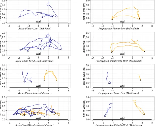
Figure 10. Bird’s eye views of the movement of participants in trials for individual (2 top lines) and pairs (2 bottom lines), under the condition Planar-Low(easiest) and SmallWorld-High (hardest). Basic is seen in the left column, and Propagation in the right column. The wall is at the bottom of each graph, the unit is the meter, and the black little circles (◦◦◦) indicate a touch interaction.

4.2.3 Distance Traveled

Individual: The amount of movement in the individual case was higher for Basic (17.9m) than for Propagation (9.2m), almost twice as much (three times in complex graphs), and the effect exists for all GRAPH× COMPLEXITYconditions (Figure 7).

Multi-user: Similarly, the distance covered by each participant when working in pairs was less with Propagation (4.6m) than Basic(9.3m), in all conditions (Figure 8).

Individual vs. Multi-user: As expected the distance traveled by participants in individual sessions is about twice that traveled by each participant in Multi-user sessions for both techniques (Figure 9-left). However, as shown inFigure 9-right, this effect is strong for Propagation for both Low and High complexity graphs, but only for Low complexity ones for Basic. This reinforces that the gain of working in pairs is less with Basic in complex graphs.

Figure 10illustrates these results with examples of participant trajectories in front of the wall. Pairs tend to divide their work spatially, with the exception of using Basic in SmallWorld-High. Nevertheless, video recording indicates that even here participants start the task by dividing the space, but as they cannot reach a solution, they start moving more around the space to verify their work, stepping back likely to get an overview. Thus, these patterns are not just due to the need to reach nodes to interact with, but also due to the nature of collaboration using Basic in complex graphs. 4.2.4 Observed Strategies

Individual: Instead of propagating from a single node, all individuals using Propagation selected one node, propagated

typ-ically one time (sometimes two), and then moved to the second to propagate, alternating between the two until they saw an intersection (two-color node). This strategy reduced the number of selected nodes and visual clutter (less propagation steps), helping them identify the shortest path as intersection points are inside it.

The strategy used for Basic was different. Participants con-sistently selected a subset of neighbors that seem to be between the two nodes, trying to reconstruct short paths moving from one node to the other. This was successful for the smaller and less complex graphs, but did not work well for the hardest condition SmallWorld-High, where participants had to consider a large number of nodes, as seen by the high error rate in this condition.

Multi-user: When performing the task in pairs, participants were again consistent in their strategy. With Propagation it was similar to the individual sessions, but now each participant took charge of one of the two nodes, and propagated alternatively (but not concurrently) until they found intersecting nodes. They coordinated this asynchronous double-propagation using verbal communication. Then, both participants reconstructed together a shorter path candidate, each taking responsibility of their own end of the propagation. In more complex graphs, they occasionally checked each other’s work (6 groups).

For Basic, participants again took charge of one node each, and tried to define paths using selections towards their partner, until they reached each other’s work area. They worked more or less independently, and in parallel, until they started finding intersection nodes. After that, for the more complex SmallWorld

graphs, they tried checking together candidate paths before making their choice (e.g. Figure 10bottom-left graph, notice movement overlap). But, pairs did not double check each other’s work in the easier Planar graphs (e.g. inFigure 10, 3rd row on the left, we see no movement overlap), which may explain the increased error rate. There was one notable strategy exception, one group decided to propagate systematically, simulating on their own the Propagation technique (which they had seen first).

4.2.5 Subjective Comments

Individual Users: Answers to the quantitative questions of the questionnaire (physical demand, visual disturbance, enjoyment) was very similar between the two TECH(p’s = 1). This is not very surprising given that we used a between-subject design for TECH. Multi-Users: After the collaborative session participants were able to directly compare the two techniques. All 16 preferred Propagation. On a 7-point Likert scale participants found that Propagation was less physically demanding (Avg=2.5, SD=1.2) than Basic (Avg=4, SD=1.6) since they were required to walk

less (p’s < 0.05). They also found Propagation more enjoyable

(Avg=5.3, SD=1.1) than Basic (Avg=4.1, SD=1.2).

Surprisingly, they also found Propagation to be less visually disturbing (Avg=2.9, SD=1.6) than Basic (Avg=4.8, SD=1.8)(p’s

< 0.05), contrary to our hypothesis. When asked to explain why

they found Propagation less visually disturbing, they explained that Propagation helped highlight paths of interest “helps to see how many possible shortest paths there are, which is very conve-nient”. Although four mentioned explicitly in their comments the existence of visual disturbance in Propagation, they commented that the visual footprint was desirable for tracking their work “it gets visually disturbing very quickly after a few propagations, but it is good to be able to see the changes when we can go back and forth with the propagation easily.”.

When asked if they preferred conducting the task individually or collaborating with a partner, participants had mixed opinions. Six out of the eight that run the individual session with Propa-gationpreferred to run the experiment in pairs with Propagation, instead of alone. As one explained “having a partner is easier be-cause there’s someone to help check whether the answer is correct or not and I don’t have to move around. However I’m not sure if doing it together is faster because sometimes communicating takes time”. Five out of eight participants that run the individual session with Basic preferred to do the task in pairs with Basic. But, as one participant explained “it happens that the other was exploring different solutions than me[parallel work], so he was disturbing me”. Thus, overall the multi-user context was been only slightly preferred than the individual context.

4.2.6 Discussion

Propagation was faster than Basic selection when identifying shortest paths, particularly in the more complex small-world graphs (confirming H1 on time). This can be explained by partic-ipants moving more with Basic, twice as much overall and three times for complex graphs (confirming H3 on movement). This is backed by subjective comments reporting less fatigue and higher preference for Propagation.

When moving from individuals to pairs, the mean time of both Propagation and Basic was faster, although this difference was not measurable overall. But there is a clear speed-up for complex graphs with Propagation, and for easy graphs with Basic (partially confirming H2 on time). These differences are likely due

to participant strategies. Individuals were fast with Propagation to begin with, and since pairs spent time coordinating and taking turns propagating, speedup due to collaboration is not visible. But as we move to more complex tasks, the cost of coordination drops compared to that of the task. On the other hand, individuals were slow with Basic, and as pairs worked in parallel first and combined their results later, this accelerated the work with simple graphs. But in more complex graphs this strategy was not effective, and collaboration did not compensate for the weakness of Basic when dealing with complex graphs.

Collaboration had an effect on accuracy. It increased when passing from individuals to pairs in Propagation (partially con-firming H2 on accuracy), particularly in the most complex graphs. Participants chose to closely coordinate their actions taking turns to avoid visual interference (supporting H3 on visual disturbance). Thus it is possible they had increased workspace awareness [14], a fact supported by the ease with which they double checked each other’s work. The colored propagation queries provided a filter to the interesting areas of the graph, that also helped participants focus more effectively on both their partner’s and their own work, leading to the unexpected subjective feeling that propagation was less visually disturbing (subjective feel contrary to H3 on visual disturbance). Surprisingly, accuracy decreased for Basic when moving to the collaborative setting. This can be explained by the adopted strategy of conducting part of the task independently, thus lacking a ”big picture”, that participants were forced to adopt in the individual case. This big picture is crucial for tasks such as shortest path identification, where dividing the task into spatial subtasks is not straightforward9.

4.2.7 Summary

The two techniques, Propagation and Basic, support collaboration and wall display interaction differently:

• Propagation is promising for individual work for the shortest path finding task, requiring little physical movement. In group work it leads to increased accuracy, but no measurable increase in speed as there is an overhead related to coordination due to its visual footprint. Thus tight coordination, combined with the technique’s highlighting of areas of interest, helped maintain an understanding of partners’ work and increased accuracy.

• The Basic technique is as accurate when dealing with simple graphs for individuals, but considerably slower. And its perfor-mance degrades with more complex graphs. More importantly, when pairs divide tasks spatially, it can lead to loss of awareness of partners’ work, resulting in loss of accuracy in collaborative work (compared to individual) when task division is not straightforward.

5

E

2: O

S

In the previous study we focused on a single controlled task that is not clearly divisible and parallelizable in its nature. Although pairs naturally took responsibility of one node, an overview of a larger area of the graph is required to correctly address the task. This is true for most low level graph analysis tasks suggested in the literature [37]. Nevertheless, studying them gives us insight as to how users can appropriate existing techniques in a collaborative manner. For example, Propagation, which quickly affected a large part of the graph, required explicit coordination. We examine, now, if this is true for other low level tasks.

9 _{For example, when choosing among shortest path candidates, considering} only the left half of paths is not enough to identify good candidates.

More specifically, we are interested in assessing Propagation, that proved more promising, as a general graph exploration tech-nique, observing if pairs can ”discover” on their own how to perform new tasks without task specific training. And in whether they adopt similar coordination strategies as in Exp 1. Thus we are less interested in recording time, and more in observing if and how pairs collaborated.

5.1 Experimental Design 5.1.1 Participants & Apparatus

We recruited 8 volunteers (4 females, 4 males) in pairs, aged 23 to 39, with normal or corrected-to-normal vision. Pairs knew each other and had taken part in Exp 1. Sessions lasted 30min, using the same apparatus as in the first experiment.

5.1.2 Tasks

Groups performed the following topology tasks [37]:

T1 Find the shortest distance between two nodes (as opposed to the shortest path as in Exp 1).

T2 Find the common neighbors of degree 2 between two nodes. T3 Find all connected components.

T4 Find an articulation point between connected components. T5 Open exploration, reporting interesting observations. 5.1.3 Graph Types

In T1 and T2 we used high complexity small-world graphs similar to Exp 1. In T1 the shortest distance was 6 and the two target nodes were separated by a physical distance of about 75% of the wall width. In T2 the two target nodes were closer (about 50% of the wall width) and had 5 common neighbors.

In T3 and T4, we combined unconnected small-world graphs (20 nodes each) of high complexity: three in T3 (60 nodes in total) and two fin T4 (40 nodes). To complicate the tasks, we tweaked the layout to get overlap between subgraphs. And in T4 we hid the articulation point connecting the subgraphs inside one of them.

The graph used in the open task T5 (similar to Figure 1) consisted of three subgraphs of different densities, and two un-connected nodes. Two subgraphs where un-connected through an articulation point, hidden within the third subgraph. These were the insights we wanted our participants to identify. The layout was tweaked so that subgraphs were not easy to separate visually. 5.1.4 Procedure

Participants were first reminded of the propagation technique, but no task specific training was given. Then the experimenter introduced the task without giving instructions on how to solve it, and participants performed the five tasks in order. Participants indicated they were done verbally, in a way similar to Experiment 1. If participants succeeded on their first trial within a timeout limit of 3000sec (5min), they moved on to the next task. If they failed, a strategy to solve the task was explained to them, and they were presented with another trial for that task. If they failed again, they were given a final trial, and then moved to the next task.

The experiment was recorded, and one experimenter took notes. A second experimenter gave instructions and logged the time (as in Exp 1). At the end, we asked participants if they had any suggestions for improving the technique, their thoughts on collaboration, and how confident they were in their answers.

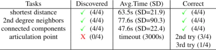
Tasks Discovered Avg.Time (SD) Correct shortest distance X (4/4) 63.5s (SD=21.9) X (4/4) 2nd degree neighbors X (4/4) 77.6s (SD=90.3) X (4/4) connected components X (4/4) 47.6s (SD=22.4) X (4/4) articulation point X (0/4) timeout (3000s) 2nd try (3/4)

3rd try (1/4) Table 3. Summary of findings for specific Tasks T1-4, indicating whether our pairs were able to discover how to perform a task, and the time it took them to do so (mean and SD). If they did not discover a strategy on their own within the timeout period, column Correct indicates on what try they succeeded.

5.2 Results

We report next participants’ success in discovering a correct strategy and time averages logged during the experiment, as well as the strategies they adopted based on video log analysis and notes taken in the experiment.

5.2.1 Discovering

All pairs discovered without any training correct strategies for identifying the shortest distance between two points, the common neighbors of degree two, and the connected components (T1-3). No pair was able to develop a correct strategy for finding an articulation point (T4), but three pairs understood how to identify possible candidates. After instruction, three pairs were able to perform a new T4 trial, and one pair on their third attempt.

All pairs conducted T1-T3 within the time limit, with con-nected component completed faster 47.6s (SD=22.4), followed by shortest distance 63.5s (SD=21.9) and 2nd degree neighbors 77.6s (SD=90.3). The larger mean time and standard deviation of 2nd degree neighbors is due to one pair that did an extensive verification of their answer (described next in strategies). We note that the times reported here include both the discussion of strategy and the actual interaction to find the solution.Table 3summarizes the discoverability of strategies and the time taken by our pairs.

In the open task, three pairs found four out of five possible insights, and one pair found all insights within the time limit. All pairs found two connected subgraphs and identified an articulation point between them. They also verified that the third subgraph was disconnected, and identified the extra disconnected nodes. One pair noticed the differences in the density of the subgraphs by calculating shortest paths.

5.2.2 Observed Strategies

We describe next the strategies adopted by participants, focusing on how they coordinated, and report their subjective comments.

Shortest Distance: In all pairs, each participant propagated from one of the two target nodes, until one or more nodes were selected by both their colors. They took turns propagating and observed each other’s work so as not to loose count of the total propagation steps performed. One pair also used the thickness of edges to confirm that bi-selected nodes were at a distance of 3 from each target node.

Common Neighbors of degree 2: All pairs propagated two levels from both target nodes and then counted the number of nodes selected in both colors. Two pairs worked independently first (propagated in parallel) and checked later the bi-colored nodes together. Of these pairs, one backtracked their propagation to verify all bi-colored nodes were neighbors of degree two exactly, rather than neighbors of degree two or less for one of the nodes. The other two took turns propagating and looking at their partner’s work, ensuring they considered neighbors of exactly degree two.