HAL Id: hal-01273842
https://hal.archives-ouvertes.fr/hal-01273842v2
Submitted on 21 Nov 2016
HAL is a multi-disciplinary open access
archive for the deposit and dissemination of sci-entific research documents, whether they are pub-lished or not. The documents may come from teaching and research institutions in France or abroad, or from public or private research centers.
L’archive ouverte pluridisciplinaire HAL, est destinée au dépôt et à la diffusion de documents scientifiques de niveau recherche, publiés ou non, émanant des établissements d’enseignement et de recherche français ou étrangers, des laboratoires publics ou privés.
Aurélien Garivier, Emilie Kaufmann, Wouter Koolen
To cite this version:
Aurélien Garivier, Emilie Kaufmann, Wouter Koolen. Maximin Action Identification: A New Bandit Framework for Games. 29th Annual Conference on Learning Theory (COLT), Jun 2016, New-York, United States. �hal-01273842v2�
Maximin Action Identification: A New Bandit Framework for Games
Aur´elien Garivier [email protected]
Institut de Math´ematiques de Toulouse; UMR5219 Universit´e de Toulouse; CNRS
UPS IMT, F-31062 Toulouse Cedex 9, France
Emilie Kaufmann [email protected]
Univ. Lille, CNRS, UMR 9189
CRIStAL - Centre de Recherche en Informatique Signal et Automatique de Lille F-59000 Lille, France
Wouter M. Koolen [email protected]
Centrum Wiskunde & Informatica, Science Park 123, 1098 XG Amsterdam, The Netherlands
Abstract
We study an original problem of pure exploration in a strategic bandit model motivated by Monte Carlo Tree Search. It consists in identifying the best action in a game, when the player may sample random outcomes of sequentially chosen pairs of actions. We propose two strategies for the fixed-confidence setting: Maximin-LUCB, based on lower- and upper- confidence bounds; and Maximin-Racing, which operates by successively eliminating the sub-optimal actions. We discuss the sample complexity of both methods and compare their performance empirically. We sketch a lower bound analysis, and possible connections to an optimal algorithm.
Keywords: multi-armed bandit problems, games, best-arm identification, racing, LUCB 1. Setting: A Bandit Model for Two-Player Zero-Sum Random Games
We study a statistical learning problem inspired by the design of computer opponents for playing games. We are thinking about two-player zero sum full information games like Checkers, Chess, Go (Silver et al.,
2016) . . . , and also games with randomness and hidden information like Scrabble or Poker (Bowling et al.,
2015). At each step during game play, the agent is presented with the current game configuration, and is tasked with figuring out which of the available moves to play. In most interesting games, an exhaustive search of the game tree is completely out of the question, even with smart pruning.
Given that we cannot consider all states, the question is where and how to spend our computa-tional effort. A popular approach is based on Monte Carlo Tree Search (MCTS) (Gelly et al., 2012;
Browne et al., 2012). Very roughly, the idea of MCTS is to reason strategically about a tractable (say up to some depth) portion of the game tree rooted at the current configuration, and to use (randomized) heuristics to estimate values of states at the edge of the tractable area. One way to obtain such estimates is by ‘rollouts’: playing reasonable random policies for both players against each other until the game ends and seeing who wins.
MCTS methods are currently applied very successfully in the construction of game playing agents and we are interested in understanding and characterizing the fundamental complexity of such ap-proaches. The existing picture is still rather incomplete. For example, there is no precise characteri-zation of the number of rollouts required to identify a close to optimal action. Sometimes, cumulated regret minimizing algorithms (e.g. UCB derivatives) are used, whereas only the simple regret is relevant
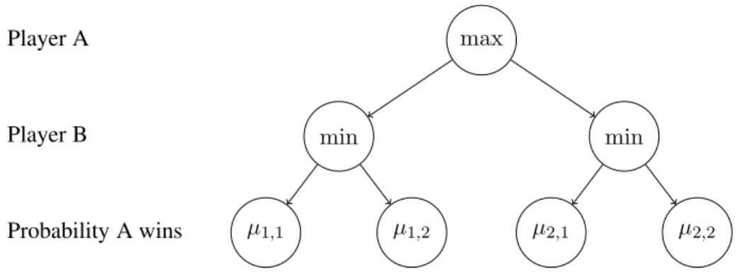
max min min µ1,1 µ1,2 µ2,1 µ2,2 Player A Player B Probability A wins
Figure 1: Game tree when there are two actions per player(K = K1= K2= 2).
here. As a first step in this direction, we investigate in this paper an idealized version of the MCTS problem for games, for which we develop a theory that leads to sample complexity guarantees.
More precisely, we study perhaps the simplest model incorporating both strategic reasoning and exploration (see Figure 1 for an example). We consider a two-player two-round zero-sum game, in which player A has K available actions. For each of these actions, indexed by i, player B can then choose among Kipossible actions, indexed by j. When player A chooses action i∈ {1, . . . , K} and then
player B chooses action j ∈ {1, . . . , Ki}, the probability that player A wins is µi,j. We investigate the
situation from the perspective of player A, who wants to identify a maximin action i∗∈ argmax
i∈{1,...,K}
min
j∈{1,...,Ki}
µi,j.
Assuming that player B is strategic and picks, whatever A’s action i, the action j minimizing µi,j, this is
the best choice for A.
The parameters of the game are unknown to player A, but he can repeatedly choose a pair P = (i, j) of actions for him and player B, and subsequently observe a sample from a Bernoulli distribution with mean µi,j. At this point we imagine the sample could be generated e.g. by a single rollout estimate in
an underlying longer game that we consider beyond tractable strategic consideration. Note that, in this learning phase, player A is not playing a game: he chooses actions for himself and for his adversary, and observes the random outcome.
The aim of this work is to propose a dynamic sampling strategy for player A in order to minimize the total number of samples (i.e. rollouts) needed to identify i∗. Denoting the possible move pairs by
P = {(i, j) ∶ 1 ≤ i ≤ K, 1 ≤ j ≤ Ki},
we formulate the problem as the search of a particular subset of arms in a stochastic bandit model with K =∑Ki=1Ki Bernoulli arms of respective expectations µP, P ∈ P. In this bandit model, parametrized
by µ= (µP)P∈P, when the player chooses an arm (a pair of actions) Ptat round t, he observes a sample
Xtdrawn under a Bernoulli distribution with mean µPt.
In contrast to best arm identification in bandit models (see, e.g.,Even-Dar et al.(2006);Audibert et al.
(2010)), where the goal is to identify the arm(s) with highest mean, argmaxP µP, here we want to
iden-tify as quickly as possible the maximin action i∗defined above. For this purpose, we adopt a sequential learning strategy (or algorithm) (Pt, τ,ˆı). Denoting by Ft = σ(X1, . . . , Xt) the sigma-field generated
• a sampling rule Pt∈ P indicating the arm chosen at round t, such that PtisFt−1measurable,
• a stopping rule τ after which a recommendation is to be made, which is a stopping time with respect toFt,
• a final guess ˆı for the maximin action i∗.
For some fixed ǫ≥ 0, the goal is to find as quickly as possible an ǫ-maximin action, with high probability. More specifically, given δ∈]0, 1[, the strategy should be δ-PAC, i.e. satisfy
∀µ, Pµ( min j∈{1...Ki∗}
µi∗,j− min
j∈{1...Kˆı}
µˆı,j≤ ǫ) ≥ 1 − δ, (1)
while keeping the total number of samples τ as small as possible. This is known, in the best-arm identifi-cation literature, as the fixed-confidence setting; alternatively, one may consider the fixed-budget setting where the total number of samples τ is fixed in advance, and where the goal is to minimize the probability that ˆı is not an ǫ-maximin action.
Related Work. Tools from the bandit literature have been used in MCTS for around a decade (see
Munos (2014) for a survey). Originally, MCTS was used to perform planning in a Markov Decision Process (MDP), which is a slightly different setting with no adversary: when an action is chosen, the transition towards a new state and the reward observed are generated by some (unknown) random pro-cess. A popular approach, UCT (Kocsis and Szepesv´ari, 2006) builds on Upper Confidence Bounds algorithms, which are useful tools for regret minimization in bandit models (e.g.,Auer et al.(2002)). In this slightly different setup (seeBubeck and Cesa-Bianchi(2012) for a survey), the goal is to maximize the sum of the samples collected during the interaction with the bandit, which amounts in our setting to favor rollouts for which player A wins (which is not important in the learning phase). This situation is from a certain perspective a little puzzling and arguably confusing, because as shown byBubeck et al.
(2011), regret minimization and best arm identification are incompatible objectives in the sense that no algorithm can simultaneously be optimal for both.
More recently, tools from the best-arm identification literature have been used by Szorenyi et al.
(2014) in the context of planning in a Markov Decision Process with a generative model. The proposed algorithm builds on the UGapE algorithm ofGabillon et al.(2012) to decide for which action new tra-jectories in the MDP starting from this action should be simulated. Just like a best arm identification algorithm is a building block for such more complex algorithms to perform planning in an MDP, we believe that understanding the maximin action identification problem is a key step towards more gen-eral algorithms in games, with provable sample complexity guarantees. For example, an algorithm for maximin action identification may be useful for planning in a competitive Markov Decision Processes (Filar and Vrieze,1996) that models stochastic games.
Contributions. In this paper, we propose two algorithms for maximin action identification in the fixed-confidence setting, whose sample complexity is presented in Section2. These algorithms are inspired by the two dominant approaches used in best arm identification algorithms. Our first algorithm, Maximin-LUCB, is described in Section 3: it relies on the use of Lower and Upper Confidence Bounds. The second, Maximin-Racing, is described in Section4: it proceeds by successive elimination of sub-optimal arms. We prove that both algorithms are δ-PAC, and give upper bounds on their sample complexity. Our analysis contrasts with that of classical BAI procedures, and exhibits unexpected elements that are specific to the game setting. Along the way, we also propose some avenues of improvement that are
illustrated empirically in Section 5. Finally, we propose in Section 6 for the two-action case a lower bound on the sample complexity of any δ-PAC algorithm, and sketch a strategy that may be optimal with respect to this lower bound. Most proofs are deferred to the Appendix.
2. Notation and Summary of the Results
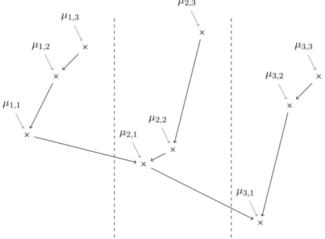
To ease the notation, in the rest of the paper we assume that the actions of the two players are re-ordered so that for each i, µi,j is increasing in j, and µi,1 is decreasing in i (so that i∗ = 1 and µ∗ = µ1,1).
These assumptions are illustrated in Figure2. With this notation, the action ˆı is an ǫ-maximin action if µ1,1−µˆı,1≤ ǫ. We also introduce Pi={(i,j),j ∈ {1,... ,Ki}} as the group of arms related to the choice
of action i for player A.
× µ1,1 × µ1,2 × µ1,3 × µ2,1 × µ2,2 × µ2,3 × µ3,1 × µ3,2 × µ3,3
Figure 2: Example ‘normal form’ mean configuration. Arrows point to smaller values. We propose in the paper two algorithms with a sample complexity of order Eµ[τ] ≃ H
∗(µ)log(1/δ), where H∗(µ) ∶= ∑ (1,j)∈P1 1 (µ1,j− µ2,1)2 +(i,j)∈P∖P∑ 1 1
(µ1,1− µi,1)2∨(µi,j− µi,1)2
. This complexity term is easy to interpret:
• each arm (1,j) in the optimal group P1 should be drawn enough to be discriminated from µ2,1
(roughly of order(µ1,j− µ2,1)−2log(1/δ) times)
• each other arm(i,j) in P∖P1should be drawn enough to either be discriminated from the smallest
arm in the same group, µi,1, or so that µi,1is discriminated from µ1,1.
Our Theorems4and 8respectively lead to (asymptotic) upper bounds featuring two complexity terms H1∗(µ) and H2∗(µ) that are very close to H∗(µ). When there are two actions per player, Theorem 5
shows that the sample complexity of M-LUCB is asymptotically upper bounded by 16H∗(µ)log(1/δ). We discuss sample complexity lower bounds and their connection to future algorithms in Section6.
It is to be noted that such a sample complexity cannot be attained by a naive use of algorithms for best arm identification. Indeed the most straightforward idea would be to follow the tree structure bottom-up; recursively identifying alternately best and worst arms. For two levels, we would first perform worst-arm identification on j for each i, followed by best-arm identification on the obtained set of worst arms. To see why such modular approaches fail, recall that the sample complexity of best and worst arm identification scales with the sum of the inverse squared gaps (see e.g.Kalyanakrishnan et al.(2012)). But many of these gaps, however small, are irrelevant for finding i∗. For a simple example consider µ1,1 = µ1,2 ≫
µ2,1 = µ2,2. Hierarchical algorithms find such equal means (zero gap) within actions arbitrarily hard,
while our methods fare fine: only the large gap between actions appears in our complexity measure H∗. We now explain in Section 3and4 how to carefully use best arm identification tools to come up with algorithms whose sample complexity scales with H∗(µ).
3. First Approach: M-LUCB
We first describe a simple strategy based on confidence intervals, called Maximin-LUCB (M-LUCB). Confidence bounds have been successfully used for best-arm identification in the fixed-confidence setting (Kalyanakrishnan et al.,2012;Gabillon et al.,2012;Jamieson et al.,2014). The algorithm proposed in this section for maximin action identification is inspired by the LUCB algorithm ofKalyanakrishnan et al.
(2012), based on Lower and Upper Confidence Bounds.
For every pair of actions P ∈ P, let IP(t) = [LP(t),UP(t)] be a confidence interval on µP built
using observations from arm P gathered up to time t. Such a confidence interval can be obtained by using the number of draws NP(t) ∶= ∑ts=11(Ps=P )and the empirical mean of the observations for this
pair ˆµP(t) ∶= ∑ts=1Xs1(Ps=P )/NP(t) (with the convention ˆµP(0) = 0). The M-LUCB strategy aims
at aligning the lower confidence bounds of arms that are in the same groupPi. Arms to be drawn are
chosen two by two: for any even time t, defining for every i∈{1,... ,K} ci(t) = argmin
1≤j≤Ki
L(i,j)(t) and ˆı(t) = argmax
1≤i≤K
min
1≤j≤Ki
ˆ µi,j(t) ,
the algorithm draws at rounds t+ 1 and t + 2 the arms Pt+1= Htand Pt+2= Stwhere
Ht=(ˆı(t),cˆı(t)(t)) and St= argmax P∈{(i,ci(t))}i≠ˆı
UP(t).
This is indeed a regular LUCB sampling rule on a time-dependent set of arms each representing one action: {(i,ci(t))}i∈{1,...,K}. When there are two actions for each player, one may alternatively draw at
each time t the arm Pt+1= argminP∈{Ht,St}NP(t) only.
The stopping rule, which depends on the parameter ǫ≥ 0 (that can be set to zero if µ1,1> µ2,1) is
τ = inf{t ∈ 2N ∶ LHt(t) > USt(t) − ǫ} . (2)
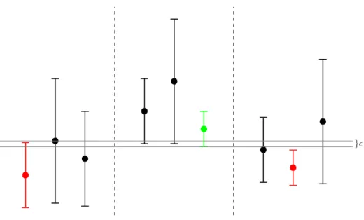
Then arm ˆı= ˆı(τ), the empirical maximin action at that time, is recommended to player A. The stopping rule is illustrated in Figure 3. The choice of the representative arms {(i,ci(t))i∈{1,...,K} is
crucial, and it can be understood from the proof of Lemma11in Appendix Awhy aligning the lower confidence bounds inside each action is a good idea.
}ǫ
Figure 3: Stopping rule (2). The algorithm stops because the lower bound of the green arm beats up to slack ǫ the upper bound for at least one arm (marked red) in each other action, the one with smallest LCB. In this case action ˆı= 2 is recommended.
3.1. Analysis of the Algorithm
We analyze the algorithm under the assumptions µ1,1 > µ2,1and ǫ= 0. We consider the Hoeffding-type
confidence bounds LP(t) = ˆµP(t) − ¿ Á Á À β(t,δ) 2NP(t) and UP(t) = ˆµP(t) + ¿ Á Á À β(t,δ) 2NP(t) , (3)
where β(t,δ) is some exploration rate. A choice of β(t,δ) that ensures the δ-PAC property (1) is given below. In order to highlight the dependency of the stopping rule on the risk level δ, we denote it by τδ.
Theorem 1 Let H1∗(µ) = K1 ∑ j=1 1 (µ1,j−µ 1,1+µ2,1 2 ) 2 + ∑ (i,j)∈P∖P1 1 (µ1,1+µ2,1 2 − µi,1) 2 ∨(µi,j− µi,1)2 . On the event E = ⋂ P∈Pt∈2N⋂ {µ P ∈[LP(t),UP(t)]} ,
the M-LUCB strategy returns the maximin action and uses a total number of samples upper-bounded by T(µ,δ) = inf {t ∈ N ∶ 4H1∗(µ)β(t,δ) < t}.
According to Theorem1, the exploration rate should be large enough to control Pµ(E), and as small as
possible so as to minimize T(µ,δ). The self-normalized deviation bound of Capp´e et al.(2013) gives a first solution (Corollary 2), whereas Lemma 7 ofKaufmann et al.(2015) yields Corollary3. In both cases, explicit bounds on T(µ,δ) are obtained using the technical Lemma12stated in AppendixA.
Corollary 2 Letα> 0 and C = Cαbe such that eK ∞ ∑ t=1 (log t)(log(Ct1+α)) t1+α ≤ C ,
and letδ satisfy 4(1 + α)(C/δ)1/(1+α) > 4.85. With probability larger than 1 − δ, the M-LUCB strategy using the exploration rate
β(t,δ) = log (Ct
1+α
δ ) , (4)
returns the maximin action within a number of steps upper-bounded as
τδ≤ 4(1+α)H1∗(µ) ⎡⎢ ⎢⎢ ⎢⎣log( 1 δ) + log(C(4(1 + α)H ∗ 1(µ))1+α) + 2(1 + α)log log ⎛ ⎝ 4(1 + α)H1∗(µ)C1+1α δ1+1α ⎞ ⎠ ⎤⎥ ⎥⎥ ⎥⎦. Corollary 3 Forb, c such that c> 2 and b > c/2, let the exploration rate be
β(t,δ) = log1 δ + b log log 1 δ + c log log(et) and let fb,c(δ) = K√e π2 3 1 8c/2
(√log(1/δ) + blog log(1/δ) + 2√2)c
(log(1/δ))b .
With probability larger than 1− fb,c(δ)δ, M-LUCB returns the maximin action and, for some positive
constantCc and forδ small enough,
τδ≤ 4H1∗(µ)[log ( 1 δ) + log(8CcH ∗ 1(µ)) + 2log log ( 8CcH1∗(µ) δ )] .
Elaborating on the same ideas, it is possible to obtain results in expectation, at the price of a less explicit bound, that holds for a slightly larger exploration rate.
Theorem 4 The M-LUCB algorithm usingβ(t,δ) defined by (4), with α> 1, is δ-PAC and satisfies lim sup δ→0 Eµ[τδ] log(1/δ) ≤ 4(1 + α)H ∗ 1(µ).
H1∗(µ) is very close to the quantity H∗(µ) introduced in Section2. The difference is that in H1∗(µ) µi,1 and µ1,1 need to be discriminated from a ‘virtual arm’ with mean(µ1,1+ µ2,1)/2 in place of µ1,1
and µ2,1 respectively. We view this virtual arm (that corresponds to the choice of a parameter c in
AppendixA) as an artifact of our proof. In the particular case of two actions per player, we propose the following finer result, that holds for the variant of M-LUCB that samples the least drawn arm among Ht
and Stat round t+ 1.
Theorem 5 AssumeK= K1= K2= 2. The M-LUCB algorithm using β(t,δ) defined by (4) with α> 1
isδ-PAC and satisfies
lim sup
δ→0
Eµ[τδ]
log(1/δ) ≤ 8(1 + α)H
3.2. Improved Intervals and Stopping Rule
The symmetry and the simple form of the sub-gaussian confidence intervals (3) are convenient for the analysis, but they can be greatly improved thanks to better deviation bounds for Bernoulli distributions. A simple improvement (seeKaufmann and Kalyanakrishnan(2013)) is to use Chernoff confidence inter-vals, based on the binary relative entropy function d(x,y) = xlog(x/y) + (1 − x)log((1 − x)/(1 − y)). Moreover, the use of a better stopping rule based on generalized likelihood ratio tests (GLRT) has been proposed recently for best-arm identification, leading to significant improvements. We propose here an adaptation of the Chernoff stopping rule ofGarivier and Kaufmann(2016), valid for the case ǫ= 0.
Our stopping rule is based on the statistic:
ZP,Q(t) ∶= log maxµ′ P≥µ ′ Qpµ ′ P (X P NP(t))pµ ′ Q(X Q NQ(t)) maxµ′ P≤µ ′ Qpµ ′ P (X P NP(t))pµ ′ Q(X Q NQ(t)) ,
where XPs is a vector that contains the first s observations of arm P and pµ(Z1, . . . , Zs) is the likelihood
of the given s observations from an i.i.d. Bernoulli distribution with mean µ. Introducing the empirical mean of the combined samples from arms P and Q,
ˆ µP,Q(t) ∶= NP(t) NP(t) + NQ(t) ˆ µP(t) + NQ(t) NP(t) + NQ(t) ˆ µQ(t),
it appears that for ˆµP(t) ≥ ˆµQ(t),
ZP,Q(t) = NP(t)d(ˆµP(t), ˆµP,Q(t)) + NQ(t)d(ˆµQ(t), ˆµP,Q(t)) ,
and ZP,Q(t) = −ZQ,P(t). The stopping rule is defined as
τ = inf{t ∈ N ∶ ∃i ∈ {1,... ,K} ∶ ∀i′≠ i, ∃j′∈{1,... ,Ki′} ∶ ∀j ∈ {1,... ,Ki},Z
(i,j),(i′,j′)(t) > β(t,δ)}
= inf{t ∈ N ∶ max
i∈{1,...,K}mini′≠i max
j′∈{1,...,K i′}
min
j∈{1,...,Ki}
Z(i,j),(i′,j′)(t) > β(t,δ)} . (5)
Proposition 6 Using the stopping rule (5) with the exploration rate β(t,δ) = log (2K1(K−1)t
δ ), whatever
the sampling rule, ifτ is a.s. finite, the recommendation is correct with probability Pµ(ˆı= i
∗) ≥ 1 − δ.
Sketch of Proof. Recall that in our notation the optimal action is i∗= 1. P µ(ˆı≠ 1) ≤ Pµ(∃t ∈ N,∃i ∈ {2,... ,K},∃j ′∈{1,... ,K 1},Z(i,1),(1,j′)(t) > β(t,δ)) ≤ ∑K i=2 K1 ∑ j′=1 Pµ(∃t ∈ N,Z(i,1),(1,j′)(t) > β(t,δ)) .
Note that for i ≠ 1, µi,1 < µ1,j′ for all j′ ∈ {1,... ,K1}. The result follows from the following bound
proved inGarivier and Kaufmann(2016): whenever µP < µQ, for any sampling strategy,
P
µ(∃t ∈ N ∶ ZP,Q(t) ≥ log (
2t
4. Second Approach: A Racing Algorithm
We now propose a Racing-type algorithm for the maximin action identification problem, inspired by another line of algorithms for best arm identification (Maron and Moore,1997;Even-Dar et al., 2006;
Kaufmann and Kalyanakrishnan,2013). Racing algorithms are simple and powerful methods that pro-gressively concentrate on the best actions. We give in this section an analysis of a Maximin-Racing algorithm that relies on the refined information-theoretic tools introduced in the previous section. 4.1. A Generic Maximin-Racing Algorithm
The Maximin Racing algorithm maintains a set of active armsR and proceeds in rounds, in which all the active arms are sampled. At the end of round r, all active arms have been sampled r times and some arms may be eliminated according to some elimination rule. We denote by ˆµP(r) the average of the r
observations on arm P . The elimination rule relies on an elimination function f(x,y) (f(x,y) is large if x is significantly larger than y), and on a threshold function β(r,δ).
The Maximin-Racing algorithm presented below performs two kinds of eliminations: the largest arm in each setRimay be eliminated if it appears to be significantly larger than the smallest arm inRi(high
arm elimination), and the group of armsRicontaining the smallest arm may be eliminated (all the arms
inRiare removed from the active set) if it contains one arm that appears significantly smaller than all
the arms of another groupRj (action elimination).
Maximin Racing Algorithm.
Parameters. Elimination function f , threshold function β
Initialization. For each i∈{1,... ,K},Ri = Pi, andR ∶= R1∪ ⋅ ⋅ ⋅ ∪ RK.
Main Loop.At round r:
• all arms inR are drawn, empirical means ˆµP(r), P ∈ R are updated
• High arms elimination step: for each action i= 1 . . . K, if∣Ri∣ ≥ 2 and
rf(max P∈Ri ˆ µP(r), min P∈Ri ˆ µP(r)) ≥ β(r,δ) , (7)
then remove Pm= argmax P∈Ri
ˆ
µP(r) from the active set : Ri= Ri/{Pm}, R = R/{Pm}.
• Action elimination step: if(˜ı, ˜) = argmin
P∈R ˆ µP(r) and if rf(max i≠˜ı Pmin∈Ri ˆ µP(r), ˆµ(˜ı,˜)(r)) ≥ β(r,δ) ,
then remove ˜ı from the possible maximin actions:R = R/R˜ıandR˜ı= ∅.
The algorithm stops when all but one of theRi are empty, and outputs the index of the remaining set as
the maximin action. If the stopping condition is not met at the end of round r= r0 ∶=
2 ǫ2log(
4K δ ),
4.2. Tuning the Elimination and Threshold Functions
In the best-arm identification literature, several elimination functions have been studied. The first idea, presented in the Successive Elimination algorithm ofEven-Dar et al.(2006), is to use the simple differ-ence f(x,y) = (x − y)21(x≥y); in order to take into account possible differences in the deviations of the
arms, the KL-Racing algorithm ofKaufmann and Kalyanakrishnan (2013) uses an elimination function equivalent to f(x,y) = d∗(x,y)1(x≥y), where d∗(x,y) is defined as the common value of d(x,z) and
d(y,z) for the unique z satisfying d(x,z) = d(y,z). In this paper, we use the divergence function f(x,y) = I(x,y) ∶= [d(x,x + y
2 ) + d(y, x + y
2 )]1(x≥y) (8)
inspired by the deviation bounds of Section3.2. In particular, using again Inequality (6) for the uniform sampling rule yields, whenever µP < µQ,
Pµ(∃r ∈ N ∶ rI(ˆµP(r), ˆµQ(r)) ≥ log2r
δ ) ≤ δ. (9)
Using this bound, Proposition7 (proved in AppendixB.1) proposes a choice of the threshold function for which the Maximin-Racing algorithm is δ-PAC.
Proposition 7 With the elimination function I(x,y) of Equation (8) and with the threshold function β(t,δ) = log (4CKt/δ), the Maximin-Racing algorithm satisfies
Pµ(µ1,1−µˆı,1≤ ǫ) ≥ 1 − δ,
withCK≤(K)2. Ifµ1,1> µ1,2and if ∀i, µi,1< µi,2, then we may takeCK= K × maxiKi.
4.3. Sample Complexity Analysis
We propose here an asymptotic analysis of the number of draws of each arm(i,j) under the Maximin-Racing algorithm, denoted by τδ(i,j). These bounds are expressed with the deviation function I, and
hold for ǫ> 0. For ǫ = 0, one can provide similar bounds under the additional assumption that all arms are pairwise distinct.
Theorem 8 Assume µ1,1 > µ2,1. For every ǫ > 0, and for β(t,δ) chosen as in Proposition 7, the
Maximin-Racing algorithm satisfies, for everyj∈{1,... ,K1},
lim sup δ→0 Eµ[τδ(1,j)] log(1/δ) ≤ 1 max(ǫ2/2,I(µ 1,1, µ2,1),I(µ1,j, µ1,1)))
and, for any(i,j) ∈ P ∖ P1,
lim sup δ→0 E µ[τδ(i,j)] log(1/δ) ≤ 1 max(ǫ2/2,I(µ
i,1, µ1,1),I(µi,j, µi,1))
.
It follows from Pinsker’s inequality that I(x,y) > (x − y)2, and hence Theorem8implies in particular that for the M-Racing algorithm (for a sufficiently small ǫ) lim supδ→0E
µ[τδ]/log(1/δ) ≤ H ∗ 2(µ), where H2∗(µ) ∶= K1 ∑ j=1 1 (µ1,j−µ1,1)2∨(µ1,1−µ2,1)2 + ∑ (i,j)∈P∖P1 1
(µ1,1−µi,1)2∨(µi,j−µi,1)2
The complexity term H2∗(µ) is very close to the quantities H∗(µ) and H1∗(µ) respectively intro-duced in Section2 and Theorem1. The terms corresponding to arms inP ∖ P1 are identical to those
in H∗(µ) and strictly smaller than those in H1∗(µ) (since no ‘virtual arm’ (µ1,1+µ2,1)/2 has been
introduced in the analysis of M-Racing). However, the terms corresponding to the arms(1,j),j ≥ 2 are strictly larger than those in H∗(µ) (as (µ1,j−µ1,1) ∨ (µ1,1−µ2,1) is strictly smaller than (µ1,j−µ2,1)),
and can even be larger than those in H1∗(µ). But this is mitigated by the fact that there is no multi-plicative constant in front of the complexity term H2∗(µ). Besides, as Theorem8involves the deviation function I(x,y) = d(x,(x + y)/2) + d(y,(x + y)/2 and not a subgaussian approximation, the resulting upper bound on the sample complexity of M-Racing can indeed be significantly better.
5. Numerical Experiments and Discussion
In the previous sections, we have proposed two different algorithms for the maximin action identification problem. The analysis that we have given does not clearly advocate the superiority of one or the other. The goal of this section is to propose a brief numerical comparison in different settings, and to compare with other possible strategies.
We will notably study empirically two interesting variants of M-LUCB. The first improvement that
we propose is the M-KL-LUCB strategy, based on KL-based confidence bounds (Kaufmann and Kalyanakrishnan
(2013)). The second variant, M-Chernoff, additionally improves the stopping rule as presented in Sec-tion3.2. Whereas Proposition6justifies the use of the exploration rate β(t,δ) = log(4K2t/δ), which is over-conservative in practice, we use β(t,δ) = log((log(t) + 1)/δ) in all our experiments, as suggested by Corollary3(this appears to be already quite a conservative choice in practice). In the experiments, we set δ= 0.1, ǫ = 0.
To simplify the discussion and the comparison, we first focus on the particular case in which there are two actions for each player. As an element of comparison, one can observe that finding i∗is at most as hard as finding the worst arm (or the three best) among the four arms(µi,j)1≤i,j≤2. Thus, one could
use standard best-arm identification strategies like the (original) LUCB algorithm. For the latter, the complexity is of order 2 (µ1,1−µ2,1)2 + 1 (µ1,2−µ2,1)2 + 1 (µ2,2−µ2,1)2 ,
which is much worse than the complexity term obtained for M-LUCB in Theorem 5 when µ2,2 and
µ2,1are close to one another. This is because a best arm identification algorithm does not only find the
maximin action, but additionally figures out which of the arms in the other action is worst. Our algorithm does not need to discriminate between µ2,1and µ2,2, it only tries to assess that one of these two arms is
smaller than µ1,1. However, for specific instances in which the gap between µ2,2and µ2,1 is very large,
the difference vanishes. This is illustrated in the numerical experiments of Table1, which involve the following three sets of parameters (the entry(i,j) in each matrix is the mean µi,j):
µ1=[ 0.4 0.5 0.3 0.35 ] µ2=[ 0.4 0.5 0.3 0.45 ] µ3=[ 0.4 0.5 0.3 0.6 ] (10)
We also perform experiments in a model with 3 × 3 actions with parameters:
µ= ⎡⎢ ⎢⎢ ⎢⎢ ⎣ 0.45 0.5 0.55 0.35 0.4 0.6 0.3 0.47 0.52 ⎤⎥ ⎥⎥ ⎥⎥ ⎦ (11)
τ1,1 τ1,2 τ2,1 τ2,2 τ1,1 τ1,2 τ2,1 τ2,2 τ1,1 τ1,2 τ2,1 τ2,2 M-LUCB 1762 198 1761 462 1761 197 1760 110 1755 197 1755 36 M-KL-LUCB 762 92 733 237 743 92 743 54 735 93 740 16 M-Chernoff 315 59 291 136 325 61 327 41 321 61 326 13 M-Racing 324 152 301 298 329 161 318 137 322 159 323 35 KL-LUCB 351 64 3074 2768 627 83 841 187 684 88 774 32
Table 1: Number of draws of the different arms under the models (10) parameterized by µ1, µ2, µ3
(from left to right), averaged over N = 10000 repetitions
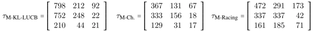
Figure4shows that the best three algorithms in the previous experiments behave as expected: the num-ber of draws of the arms are ordered exactly as suggested by the bounds given in the analysis. These
τM-KL-LUCB= ⎡⎢ ⎢⎢ ⎢⎢ ⎣ 798 212 92 752 248 22 210 44 21 ⎤⎥ ⎥⎥ ⎥⎥ ⎦ τM-Ch.= ⎡⎢ ⎢⎢ ⎢⎢ ⎣ 367 131 67 333 156 18 129 31 17 ⎤⎥ ⎥⎥ ⎥⎥ ⎦ τM-Racing = ⎡⎢ ⎢⎢ ⎢⎢ ⎣ 472 291 173 337 337 42 161 185 71 ⎤⎥ ⎥⎥ ⎥⎥ ⎦ Figure 4: Number of draws of each arm under the bandit model (11), averaged of N = 10000 repetitions
experiments tend to show that, in practice, the best two algorithms are M-Racing and M-Chernoff, with a slight advantage for the latter. However, we did not provide theoretical sample complexity bounds for M-Chernoff, and it is to be noted that the use of Hoeffding bounds in the M-LUCB algorithm (that has been analyzed) is a cause of sub-optimality. Among the algorithms for which we provide theoretical sample complexity guarantees, the M-Racing algorithm appears to perform best.
6. Perspectives
To finish, let us sketch the (still speculative) perspective of an important improvement. For simplicity, we focus on the case where each player chooses among only two possible actions, and we change our notation, using: µ1 ∶= µ1,1, µ2 ∶= µ1,2, µ3 ∶= µ2,1, µ4 ∶= µ2,2. As we will see below, the optimal strategy
is going to depend a lot on the position of µ4 relatively to µ1 and µ2. Given w =(w1, . . . , w4) ∈ ΣK =
{w ∈ R4
+∶w1+ ⋅ ⋅ ⋅ +w4= 1}, we define for a,b,c in {1,... ,4}:
µa,b(w) = waµa+wbµb wa+wb and µa,b,c(w) = waµa+wbµb+wcµc wa+wb+wc .
Using a similar argument than the one of Garivier and Kaufmann(2016) in the context of best-arm identification, one can prove the following (non explicit) lower bound on the sample complexity. Theorem 9 Anyδ-PAC algorithm satisfies
E
µ[τδ] ≥ T
where T∗(µ)−1 ∶= sup w∈ΣK inf µ′∶µ′1∧µ ′ 2<µ ′ 3∧µ ′ 4 (∑K a=1 wad(µa, µ′a)) = sup w∈ΣK F(µ,w), (12)
whereF(µ,w) = min[F1(µ,w),F2(µ,w)], with
Fa(µ,w) = {
wad(µa, µa,3(w)) + w3d(µ3, µa,3(w)) ifµ4≥ µa3(w) ,
wad(µa, µa,3,4(w)) + w3d(µ3, µa,3,4(w)) + w4d(µ4, µa,3,4(w)) otherwise.
A particular case. When µ4 > µ2, for any w ∈ ΣK it holds that µ4 ≥ µ1,3(w) and µ4 ≥ µ2,3(w).
Hence the complexity term can be rewritten to T∗(µ)−1= sup
w∈ΣK
min
a=1,2wad(µa, µa,3(w)) + w3d(µ3, µa,3(w)) .
In that case it is possible to show that the following quantity, w∗(µ) = argmax
w∈ΣK
min
a=1,2wad(µa, µa,3(w)) + w3d(µ3, µa,3(w))
is unique and to give an explicit expression. This quantity is to be interpreted as the vector of proportions of draws of the arms by a strategy matching the lower bound. In this particular case, one finds w4∗(µ) = 0, showing that an optimal strategy could draw arm 4 only an asymptotically vanishing proportion of times as δ and ǫ go to 0.
Towards an Asymptotically Optimal Algorithm. Assume that the solution of the general optimiza-tion problem (12) is well-behaved (unicity of the solution, continuity in the parameters, . . . ) and that we can find an efficient algorithm to compute, for any given µ,
w∗(µ) = argmax
w∈ΣK
min[F1(µ,w),F2(µ,w)].
Letting Alt(µ) = {µ′∶i∗(µ) ≠ i∗(µ′)}, one can introduce ˆ Z(t) ∶= inf µ′∈Alt( ˆµ(t)) K ∑ a=1 Na(t)d(ˆµa(t),µ′a) = tF((Na(t)/t)a=1...4, ˆµ(t)) = logmaxµ′∉Alt( ˆµ(t))pµ′(X1, . . . , Xt)
maxµ′∈Alt( ˆµ(t))p
µ′(X1, . . . , Xt)
,
where pµ′(X1, . . . , Xt) is the likelihood of the observations up to time t under the model parametrized
by µ′∈[0,1]4. Then, if we can design a sampling rule ensuring that for all a, Na(t)/t tends to w∗a(µ),
and if we combine it with the stopping rule
τδ= inf{t ∈ N ∶ ˆZ(t) > log(Ct/δ)}
for some positive constant C, then one can prove the following: lim sup
δ→0
Eµ[τδ] log(1/δ) ≤ T
∗(µ).
But proving that this stopping rule does ensures a δ-PAC algorithm is not straightforward, and the anal-ysis remains to be done.
Acknowledgments
This work was partially supported by the CIMI (Centre International de Math´ematiques et d’Informa-tique) Excellence program while Emilie Kaufmann visited Toulouse in November 2015. Garivier and Kaufmann acknowledge the support of the French Agence Nationale de la Recherche (ANR), under grants ANR-13-BS01-0005 (project SPADRO) and ANR-13-CORD-0020 (project ALICIA). Koolen acknowledges support from the Netherlands Organization for Scientific Research (NWO) under Veni grant 639.021.439.
References
J-Y. Audibert, S. Bubeck, and R. Munos. Best Arm Identification in Multi-armed Bandits. In Proceedings of the 23rd Conference on Learning Theory, 2010.
P. Auer, N. Cesa-Bianchi, and P. Fischer. Finite-time analysis of the multiarmed bandit problem. Machine Learning, 47(2):235–256, 2002.
M. Bowling, N. Burch, M. Johanson, and O. Tammelin. Heads-up limit hold’em poker is solved. Science, 347(6218):145–149, January 2015.
C. Browne, E. Powley, D. Whitehouse, S. Lucas, P. Cowling, P. Rohlfshagen, S. Tavener, D. Perez, S. Samothrakis, and S. Colton. A survey of monte carlo tree search methods. IEEE Transactions on Computational Intelligence and AI in games,, 4(1):1–49, 2012.
S. Bubeck and N. Cesa-Bianchi. Regret analysis of stochastic and nonstochastic multi-armed bandit problems. Fondations and Trends in Machine Learning, 5(1):1–122, 2012.
S. Bubeck, R. Munos, and G. Stoltz. Pure Exploration in Finitely Armed and Continuous Armed Bandits. Theoretical Computer Science 412, 1832-1852, 412:1832–1852, 2011.
O. Capp´e, A. Garivier, O-A. Maillard, R. Munos, and G. Stoltz. Kullback-Leibler upper confidence bounds for optimal sequential allocation. Annals of Statistics, 41(3):1516–1541, 2013.
E. Even-Dar, S. Mannor, and Y. Mansour. Action Elimination and Stopping Conditions for the Multi-Armed Bandit and Reinforcement Learning Problems. Journal of Machine Learning Research, 7: 1079–1105, 2006.
J. Filar and K. Vrieze. Competitive Markov Decision Processes. Springer, 1996.
V. Gabillon, M. Ghavamzadeh, and A. Lazaric. Best Arm Identification: A Unified Approach to Fixed Budget and Fixed Confidence. In Advances in Neural Information Processing Systems, 2012.
Aur´elien Garivier and Emilie Kaufmann. Optimal best arm identification with fixed confidence. In Proceedings of the 29th Conference On Learning Theory (to appear), 2016.
S. Gelly, L. Kocsis, M. Schoenauer, M. Sebag, D. Silver, C. Szepesv´ari, and O. Teytaud. The grand challenge of computer go: Monte carlo tree search and extensions. Commun. ACM, 55(3):106–113, 2012.
K. Jamieson, M. Malloy, R. Nowak, and S. Bubeck. lil’UCB: an Optimal Exploration Algorithm for Multi-Armed Bandits. In Proceedings of the 27th Conference on Learning Theory, 2014.
S. Kalyanakrishnan, A. Tewari, P. Auer, and P. Stone. PAC subset selection in stochastic multi-armed bandits. In International Conference on Machine Learning (ICML), 2012.
E. Kaufmann and S. Kalyanakrishnan. Information complexity in bandit subset selection. In Proceeding of the 26th Conference On Learning Theory., 2013.
E. Kaufmann, O. Capp´e, and A. Garivier. On the Complexity of Best Arm Identification in Multi-Armed Bandit Models. Journal of Machine Learning Research (to appear), 2015.
L. Kocsis and C. Szepesv´ari. Bandit based monte-carlo planning. In Proceedings of the 17th European Conference on Machine Learning, ECML’06, pages 282–293, Berlin, Heidelberg, 2006. Springer-Verlag. ISBN 3-540-45375-X, 978-3-540-45375-8.
O. Maron and A. Moore. The Racing algorithm: Model selection for Lazy learners. Artificial Intelligence Review, 11(1-5):113–131, 1997.
R. Munos. From bandits to Monte-Carlo Tree Search: The optimistic principle applied to optimization and planning., volume 7(1). Foundations and Trends in Machine Learning, 2014.
D. Silver, A. Huang, C. J. Maddison, A. Guez, L. Sifre, G. van den Driessche, J. Schrittwieser, I. Antonoglou, V. Panneershelvam, M. Lanctot, S. Dieleman, D. Grewe, J. Nham, N. Kalchbren-ner, I. Sutskever, T. Lillicrap, M. Leach, K. Kavukcuoglu, T. Graepel, and D. Hassabis. Mastering the game of go with deep neural networks and tree search. Nature, 529:484–489, 2016.
B. Szorenyi, G. Kedenburg, and R. Munos. Optimistic planning in markov decision processes using a generative model. In Advances in Neural Information Processing Systems, 2014.
Appendix A. Analysis of the Maximin-LUCB Algorithm
We define the event
Et= ⋂ P∈P(µ
P ∈[LP(t),UP(t)]),
so that the eventE defined in Theorem1rewritesE =⋂t∈2NEt.
Assume that the eventE holds. The arm ˆı recommended satisfies, by definition of the stopping rule (and by definition of St) that, for all i≠ ˆı
min
j∈Kˆı
L(ˆı,j)(τδ) > min j∈Ki
U(i,j)(τδ) − ǫ.
Using that LP(τδ) ≤ µP ≤ UP(τδ) for all P ∈ P (by definition of E) yields for all i
µˆı,1= min j∈Kˆı
µˆı,j> min j∈Ki
µi,j−ǫ= µi,1−ǫ,
hence maxi≠ˆıµi,1−µˆı,1 < ǫ. Thus, either ˆı = 1 or ˆı satisfies µ1,1−µˆı,1 < ǫ. In both case, ˆı is ǫ-optimal,
which proves that M-LUCB is correct onE.
Now we analyze M-LUCB with ǫ = 0. Our analysis is based on the following two key lemmas, whose proof is given below.
Lemma 10 Letc∈[µ2,1, µ1,1] and t ∈ 2N. On Et, if(τδ> t), there exists P ∈ {Ht, St} such that
(c ∈ [LP(t),UP(t)]) .
Lemma 11 Letc∈[µ2,1, µ1,1] and t ∈ 2N. On Et, for every(i,j) ∈ {Ht, St},
c∈[L(i,j)(t),U(i,j)(t)] ⇒ N(i,j)(t) ≤ min ( 2 (µi,1−c)2
, 2
(µi,j−µi,1)2)β(t,δ).
Moreover, forj∈{1,... ,K1}, one has
c∈[L(1,j)(t),U(1,j)(t)] ⇒ N(1,j)(t) ≤ 2 (µ1,j−c)2
β(t,δ). Defining, for every arm P =(i,j) ∈ P the constant
cP = 1 max[(µi,1−µ1,1+µ2 2,1) 2 ,(µi,j−µi,1)2] if P ∈ P ∖ P1, cP = 1 (µ1,j−µ1,1+µ2 2,1) 2 if P =(1,j) ∈ P1
combining the two lemmas (for the particular choice c= µ1,1+µ2 2,1) yields the following key statement: Et∩(τδ> t) ⇒ ∃P ∈ {Ht, St} ∶ NP(t) ≤ 2cPβ(t,δ). (13)
Note that H1∗(µ) = ∑P∈PcP, from its definition in Theorem1.
A.1. Proof of Theorem1
Let T be a deterministic time. On the eventE = ⋂t∈2NEt, using (13) and the fact that for every even t,
(τδ> t) = (τδ> t + 1) by definition of the algorithm, one has
min(τδ, T) = T ∑ t=11(τδ>t) = 2 ∑ t∈2N t≤T 1(τδ>t)= 2 ∑ t∈2N t≤T 1(∃P ∈{Ht,St}∶NP(t)≤2cpβ(t,δ)) ≤ 2 ∑ t∈2N t≤T ∑ P∈P 1(Pt+1=P )∪(Pt+2=P )1(NP(t)≤2cPβ(T,δ)) ≤ 4 ∑ P∈P cPβ(T,δ) = 4H1∗(µ)β(T,δ).
For any T such that 4H1∗(µ)β(T,δ) < T, one has min(τδ, T) < T, which implies τδ < T . Therefore
τδ≤ T(µ,δ) for T(µ,δ) defined in Theorem1.
A.2. Proof of Theorem4
Let γ> 0. Let T be a deterministic time. On the event GT =⋂ t∈2N ⌊γT ⌋≤t≤TEt
, one can write
min(τδ, T) = 2γT + 2 ∑ t∈2N ⌊γT ⌋≤t≤T 1(τδ>t)= 2γT + 2 ∑ t∈2N ⌊γT ⌋≤t≤T 1(∃P ∈{Ht,St}∶NP(t)≤2cpβ(t,δ)) ≤ 2γT + 2 ∑ t∈2N ⌊γT ⌋≤t≤T ∑ P∈P 1(Pt+1=P )∪(Pt+1=P )1(NP(t)≤2cPβ(T,δ)) ≤ 2γT + 4H∗ 1(µ)β(T,δ).
Introducing Tγ(µ,δ) ∶= inf{T ∈ N ∶ 4H1∗(µ)β(T,δ) < (1−2γ)T}, for all T ≥ Tγ(µ,δ), GT ⊆(τδ≤ T).
One can bound the expectation of τδin the following way (using notably the self-normalized deviation
inequality ofCapp´e et al.(2013)):
Eµ[τδ] = ∞ ∑ T=1 Pµ(τδ> T) ≤ Tγ+ ∞ ∑ T=Tγ Pµ(τδ> T) ≤ Tγ+ ∞ ∑ T=Tγ Pµ(GTc) ≤ Tγ+ ∞ ∑ T=1 T ∑ t=γTP∑∈P ⎡⎢ ⎢⎢ ⎢⎢ ⎣ Pµ⎛⎜ ⎝µP > ˆµP(t) + ¿ Á Á À β(t,δ) 2NP(t) ⎞ ⎟ ⎠+ Pµ ⎛ ⎜ ⎝µP < ˆµP(t) − ¿ Á Á À β(t,δ) 2NP(t) ⎞ ⎟ ⎠ ⎤⎥ ⎥⎥ ⎥⎥ ⎦ ≤ Tγ+ ∞ ∑ T=1 T ∑ t=γT 2KPµ ⎛ ⎜ ⎝µP > ˆµP(t) + ¿ Á Á À β(t,1) 2NP(t) ⎞ ⎟ ⎠ ≤ Tγ+ ∞ ∑ T=1 T ∑ t=γT
2Ke log(t)β(t,1)exp(−β(t,1)) ≤ Tγ+
∞
∑
T=1
2KeT log(T)β(T,1)exp(−β(γT,1)) = Tγ+
∞
∑
T=1
2KeT log(T)log(CT1+α) Cγ1+αT1+α ,
where the series is convergent for α> 1. One has Tγ(µ,δ) = inf {T ∈ N ∶ log (
CT1+α δ ) < (
1 − 2γ)T 4H1∗(µ) }.
The technical Lemma12below permits to give an upper bound on Tγ(µ,δ) for small values of δ, that
implies in particular lim sup δ→0 Eµ[τδ] log(1/δ) ≤ 4(1 + α)H1∗(µ) 1 − 2γ .
Letting γ go to zero yields the result.
Lemma 12 Ifα, c1, c2> 0 are such that a =(1 + α)c1/(1+α)2 /c1> 4.85, then
x=1 + α
c1 ( log(a) + 2log(log(a)))
is such thatc1x≥ log(c2x1+α).
Proof. One can check that if a ≥ 4.85, then log2(a) > log(a) + 2log(log(a)). Thus, y = log(a) + 2 log(log(a)) is such that y ≥ log(ay). Using y = c1x/(1 + α) and a = (1 + α)c1/(1+α)2 /c1, one obtains
the result.
A.3. Proof of Lemma10
We show that onEt∩(τδ> t), the following four statements cannot occur, which yields that the threshold
c is contained in one of the intervalsIHt(t) or ISt(t):
1. (LHt(t) > c) ∩ (LSt(t) > c)
2. (UHt(t) < c) ∩ (USt(t) < c)
3. (UHt(t) < c) ∩ (LSt(t) > c)
4. (LHt(t) > c) ∩ (USt(t) < c)
1. implies that there exists two actions i and i′such that ∀j≤ Ki, Li,j(t) ≥ c and ∀j′≤ Ki′, Li′,j′(t) ≥
c. BecauseEtholds, one has in particular µi,1 > c and µj,1 > c, which is excluded since µ1,1is the only
such arm that is larger than c.
2. implies that for all i∈{1,K}, U(i,ci(t))(t) ≤ c. Thus, in particular U(1,c1(t)) ≤ c and, as Etholds,
there exists j≤ K1 such that µ1,j < c, which is excluded.
3. implies that there exists i ≠ ˆı(t) such that minjµˆi,j(t) > ˆµHt(t) ≥ minjµˆ(ˆı(t),j)(t), which
contradicts the definition of ˆı(t).
4. implies that LHt(t) > USt(t), thus the algorithm must have stopped before the t-th round, which
is excluded since τδ> t.
We proved that there exists P ∈{Ht, St} such that c ∈ IP(t).
A.4. Proof of Lemma11
Assume that Et holds and that c ∈ [L(i,j)(t),U(i,j)(t)]. We first show that µi,1 is also contained in
[L(i,j)(t),U(i,j)(t)]. First, by definition of the algorithm, if (i,j) = Htor St, one has(i,j) = (i,ci(t)),
hence
L(i,j)(t) ≤ L(i,1)(t) ≤ µi,1,
using thatEtholds. Now, if we assume that µi,1> U(i,j)(t), because Etholds, one has µi,1> µi,j, which
is a contradiction. Thus, µi,1≤ U(i,j)(t).
As c and µi,1are both contained in[L(i,j)(t),U(i,j)(t)], whose diameter is 2
√ β(t,δ)/(2N(i,j)(t)), one has ∣c − µi,1∣ < 2 ¿ Á Á À β(t,δ) 2N(i,j)(t) ⇔ N(i,j)(t) ≤ 2β(t,δ) (µi,1−c)2 . Moreover, one can use again that L(i,j)(t) ≤ L(i,1)(t) to write
U(i,j)(t) − 2 ¿ Á Á À β(t,δ) 2N(i,j)(t) ≤ L(i,1)(t) µi,j−2 ¿ Á Á À β(t,δ) 2N(i,j)(t) ≤ µi,1, which yields N(i,j)(t) ≤ (µ2β(t,δ)i,j−µi,1)2.
If i = 1, note that ∣µ1,j −c∣ > max(∣µ1,1 −c∣,∣µ1,j −µ1,1∣). Using that c and µ1,j both belong to
I(1,j)(t)), whose diameter is 2√β(t,δ)/(2N(1,j)(t)) yield, using a similar argument as above, that for
all j∈{1,... ,K1},
N(1,j)(t) ≤
2β(t,δ) (µ1,j−c)2
.
A.5. Proof of Theorem5
In the particular case of two actions by player, we analyze the version of LUCB that draws only one arm per round. More precisely, in this particular case, letting
Xt= argmin j=1,2
L(1,j)(t) and Yt= argmin j=1,2
L(2,j)(t),
one has Pt+1= argmin P∈{Xt,Yt}
NP(t).
The analysis follows the same lines as that of Theorem4. First, we notice that the algorithm outputs the maximin action on the eventE = ∩t∈NEt, and thus the exploration rate defined in Corollary2
guaran-tees a δ-PAC algorithm. Then, the sample complexity analysis relies on a specific characterization of the draw of each of the arms given in Lemma13below (which is a counterpart of Lemma11). This result justifies the new complexity term that appears in Theorem5, as∑1≤i,j≤2c(i,j)≤ H∗(µ).
Lemma 13 On the eventE, for all P ∈ P, one has
(Pt+1= P) ∩ (τδ> t) ⊆ (NP(t) ≤ 8cPβ(t,δ)) , with c(1,1) = 1 (µ1,1−µ2,1)2 , c(1,2)= 1 (µ1,2−µ2,1)2 , c(2,1)= 1 (µ1,1−µ2,1)2 , and c(2,2) = 1 max(4(µ2,2−µ2,1)2,(µ1,1−µ2,1)2) .
Proof of Lemma13. The proof of this result uses extensively the fact that the confidence intervals in (3) are symmetric: UP(t) = LP(t) + 2 ¿ Á Á À β(t,δ) 2NP(t) .
Assume that (Pt+1 = (1,1)). By definition of the sampling strategy, one has L(1,1)(t) ≤ L(1,2)(t)
and N(1,1)(t) ≤ NYt(t). If (τδ> t), one has
L(1,1)(t) ≤ UYt(t) U(1,1)(t) − 2 ¿ Á Á À β(t,δ) 2N(1,1)(t) ≤ LYt(t) + 2 ¿ Á Á À β(t,δ) 2NYt(t) .
OnE, µ1,1≤ U(1,1)(t) and LYt(t) = min(L(2,1)(t),L(2,2)(t)) ≤ min(µ2,1, µ2,2) = µ2,1. Thus
µ1,1−µ2,1 ≤ 2 ¿ Á Á À β(t,δ) 2NYt(t) +2 ¿ Á Á À β(t,δ) 2N(1,1)(t) ≤ 4 ¿ Á Á À β(t,δ) 2N(1,1)(t),
using that N(1,1)(t) ≤ NYt(t). This proves that
(Pt+1=(1,1)) ∩ (τδ> t) ⊆ (N(1,1)(t) ≤
8β(t,δ) (µ1,1−µ2,1)2).
A very similar reasoning shows that
(Pt+1=(1,2)) ∩ (τδ> t) ⊆ (N(1,2)(t) ≤
8β(t,δ) (µ1,2−µ2,1)2).
Assume that(Pt+1=(2,1)). If (τδ> t), one has
LXt(t) ≤ U(2,1)(t) UXt(t) − 2 ¿ Á Á À β(t,δ) 2NXt(t) ≤ L(2,1)(t) + 2 ¿ Á Á À β(t,δ) 2N(2,1)(t). OnE, µ1,1≤ µXt≤ UXt(t) and L(2,1)(t) ≤ µ2,1. Thus µ1,1−µ2,1 ≤ 2 ¿ Á Á À β(t,δ) 2NXt(t) +2 ¿ Á Á À β(t,δ) 2N(2,1)(t) ≤ 4 ¿ Á Á À β(t,δ) 2N(2,1)(t), using that N(2,1)(t) ≤ NXt(t). This proves that
(Pt+1=(2,1)) ∩ (τδ> t) ⊆ (N(2,1)(t) ≤
8β(t,δ) (µ1,1−µ2,1)2).
Assume that(Pt+1=(2,2)). First, using the fact that L(2,2)(t) ≤ L(2,1)(t) yields, on E,
U(2,2)(t) − 2 ¿ Á Á À β(t,δ) 2N(2,2)(t) ≤ µ2,1 µ2,2−µ2,1 ≤ 2 ¿ Á Á À β(t,δ) 2N(2,2)(t),
which leads to N(2,2)(t) ≤ 2β(t,δ)/(µ2,2−µ2,1)2. Then, if(τδ > t), on E (using also that L(2,2)(t) ≤
L(2,1)(t)), LXt(t) ≤ U(2,2)(t) UXt(t) − 2 ¿ Á Á À β(t,δ) 2NXt(t) ≤ L(2,2)(t) + 2 ¿ Á Á À β(t,δ) 2N(2,2)(t) UXt(t) − 2 ¿ Á Á À β(t,δ) 2NXt(t) ≤ L(2,1)(t) + 2 ¿ Á Á À β(t,δ) 2N(2,2)(t) µ1,1−2 ¿ Á Á À β(t,δ) 2NXt(t) ≤ µ2,1+2 ¿ Á Á À β(t,δ) 2N(2,2)(t) µ1,1−µ2,1 ≤ 4 ¿ Á Á À β(t,δ) 2N(2,2)(t).
Thus, if µ2,2< µ1,1, one also has N(2,2)(t) ≤ 8β(t,δ)/(µ1,1−µ2,1)2. Combining the two bounds yield
(Pt+1=(2,2)) ∩ (τδ> t) ⊆ (N(2,2)(t) ≤
8β(t,δ)
max(4(µ2,2−µ2,1)2,(µ1,1−µ2,1)2))
.
Appendix B. Analysis of the Maximin-Racing Algorithm
B.1. Proof of Proposition7.
First note that for every P ∈ P, introducing an i.i.d. sequence of successive observations from arm P , the sequence of associated empirical means(ˆµP(r))r∈Nis defined independently of the arm being active.
We introduce the eventE = E1∩E2with
E1 = K ⋂ i=1(i,j)∈P⋂ i∶ µi,j=µi,1 ⋂ (i,j′ )∈Pi∶ µi,j′>µi,1 (∀r ∈ N,rf(ˆµi,j(r), ˆµi,j′(r)) ≤ β(r,δ)) E2 = ⋂ i∈{1,...,K}∶ µi,1<µ1,1 ⋂ (i,j)∈Ai∶ µi,j=µi,1 ⋂ i′ ∈{1,...,K}∶ µi′ ,1=µ1,1 ⋂ (i′,j′)∈A i′ (∀r ∈ N,rf(ˆµi,j(r), ˆµi′,j′(r)) ≤ β(r,δ))
and the event
F = ⋂
P∈P(∣ˆµ
P(r0) − µP∣ ≤
ǫ 2).
From (9) and a union bound, P(Ec) ≤ δ/2. From Hoeffding inequality and a union bound, using also the definition of r0, one has P(Fc) ≤ δ/2. Finally, Pµ(E ∩ F) ≥ 1 − δ.
We now show that onE ∩ F, the algorithm outputs an ǫ-optimal arm. On the event E, the following two statements are true for any round r≤ r0:
1. For all i, ifRi≠ ∅, then there exists(i,j) ∈ Ri such that µi,j = µi,1
2. If there exists i such thatRi≠ ∅, then there exists i′∶µi′,1= µ1,1such thatRi′≠ ∅.
Indeed, if 1. is not true, there is a non empty setRi in which all the arms in the set{(i,j) ∈ Pi ∶µi,j =
µi,1} have been discarded. Hence, in a previous round at least one of these arms must have appeared
strictly larger than one of the arms in the set{(i,j′) ∈ Pi ∶µi,j′ > µi,1} (in the sense of our elimination
rule), which is not possible from the definition ofE1. Now if 2. is not true, there exists i′∶µi′,1= µ1,1,
such that Ri′ has been discarded at a previous round by some non-empty set Ri, with µi,1 < µ1,1.
Hence, there exists(i′, j′) ∈ Ai′ that appears significantly smaller than all arms in Ri (in the sense of
our elimination rule). As Ri contains by 1. some arm µi,j with µi,j = µi,1, there exists r such that
rd(µ(i,j)(r),µ(i′,j′)(r)) > β(r,δ), which contradicts the definition of E2.
From the statements 1. and 2., onE ∩ F if the algorithm terminates before r0, using that the last set
in the raceRi must satisfy µi,1 = µ1,1, the action ˆı is in particular ǫ-optimal. If the algorithm has not
stopped at r0, the arm ˆı recommended is the empirical maximin action. LettingRi some set still in the
race with µi,1= µ1,1, one has,
min P∈Rˆı ˆ µP(r0) ≥ min P∈Ri ˆ µP(r0).
AsF holds and because there exists(ˆı, ˆ) ∈ Rˆıwith µˆı,ˆ= µˆı,1, and(i,j) ∈ Riwith µi,j= µ1,1, one has
min P∈Ri ˆ µP(r0) ≥ min P∈Ri(µ P −ǫ/2) = µi,j−ǫ/2 = µ1,1−ǫ/2. min P∈Rˆı ˆ µP(r0) ≤ min P∈Rˆı(µ P +ǫ/2) = µˆı,ˆ+ǫ/2 = µˆı,1+ǫ/2.
and thus ˆı is ǫ-optimal, since µˆı,1+ ǫ 2 ≥ µ1,1− ǫ 2 ⇔ µ1,1−µˆı,1≤ ǫ. ◻ B.2. Proof of Theorem8
Recall µ1,1 > µ2,1. We present the proof assuming additionally that for all i ∈ {1,K}, µi,1 < µi,2 (an
assumption that can be relaxed, at the cost of more complex notations).
Let α> 0. The function f defined in (8) is uniformly continuous on[0,1]2, thus there exists ηαsuch that
∣∣(x,y) − (x′, y′)∣∣
∞≤ ηα ⇒ ∣f(x,y) − f(x′, y′)∣ ≤ α.
We introduce the event
Gα,r = ⋂ P∈P(∣ˆµ
P(r) − µP∣ ≤ ηα)
and let E be the event defined in the proof of Lemma 7, which rewrites in a simpler way with our assumptions on the arms :
E =⋂K i=2 K1 ⋂ j=1(∀r ∈ N,rf(ˆµ i,1(r), ˆµ1,j(r)) ≤ β(r,δ)) K ⋂ i=1 Ki ⋂ j=2(∀r ∈ N,rf(ˆµ i,1(r), ˆµi,j(r)) ≤ β(r,δ))
Recall that on this event, arm (1,1) is never eliminated before the algorithm stops and whenever an arm (i,j) ∈ R, we know that the corresponding minimal arm (i,1) ∈ R.
Let(i,j) ≠ (1,1) and recall that τδ(i,j) is the number of rounds during which arm (i,j) is drawn.
One has
Eµ[τδ(i,j)] = Eµ[τδ(i,j)1E] + Eµ[τδ(i,j)1Ec] ≤ Eµ[τδ(i,j)1E] +
r0δ
2 . (14)
On the eventE, if arm(i,j) is still in the race at the end of round r,
• it cannot be significantly larger than(i,1): rf(ˆµi,j(r), ˆµi,1(r)) ≤ β(r,δ)
• arm(i,1) cannot be significantly smaller than (1,1) (otherwise all arms in Ri, including(i,j),
are eliminated): rf(ˆµi,1(r), ˆµ1,1(r)) ≤ β(r,δ)
Finally, one can write E µ[τδ(i,j)1E] ≤ Eµ[1E r0 ∑ r=1 1((i,j)∈R at round r)] ≤ Eµ[ r0 ∑ r=1
1(r max[f (ˆµi,j(r),ˆµi,1(r)),f (ˆµi,1(r),ˆµ1,1(r))]≤β(r,δ))]
≤ Eµ[ r0
∑
r=11(r max[f (ˆµi,j(r),ˆµi,1(r)),f (ˆµi,1(r),ˆµ1,1(r))]≤β(r,δ))1 Gα,r] + r0 ∑ r=1 P µ(G c α,r) ≤ r0 ∑ r=1
1(r(max[f (µi,j,µi,1),f (µi,1,µ1,1)]−α)≤log(4CKr/δ)+
∞ ∑ r=1 Pµ(Gα,rc ) ≤ T(i,j)(δ,α) + ∞ ∑ r=1 2K exp(−2(ηα)2r),
using Hoeffding inequality and introducing
T(i,j)(δ,α) ∶= inf {r ∈ N ∶ r (max [f(µi,j, µi,1),f(µi,1, µ1,1)] − α) > log (
4CKr
δ )}
Some algebra (Lemma12) shows that T(i,j)(δ,α) =max[f (µi,j,µi,1),f (µ1 i,1,µ1,1)]−αlog(
4CK
δ )+oδ→0(log 1 δ)
and finally, for all α> 0,
Eµ[τδ(i,j)] ≤ 1
max[f(µi,j, µi,1),f(µi,1, µ1,1)] − α
log(4CK
δ ) + o(log 1 δ) . As this holds for all α, and keeping in mind the trivial bound Eµ[τδ(i,j)] ≤ r0 =
2 ǫ2log( 4K δ ), one obtains lim sup δ→0 Eµ[τδ(i,j)] log(1/δ) ≤ 1 max[ǫ2/2,I(µ
i,j, µi,1),I(µi,1, µ1,1)]
.
To upper bound the number of draws of the arm(1,1), one can proceed similarly and write that, for all α> 0, τδ(1,1)1E = sup (i,j)∈P/{(1,1)} τδ(i,j)1E ≤ sup (i,j)∈P/{(1,1)} r0 ∑ r=1
1(r max[f (ˆµi,j(r),ˆµi,1(r)),f (ˆµi,1(r),ˆµ1,1(r))]≤β(r,δ))
≤ sup
(i,j)∈P/{(1,1)} r0
∑
r=11(r(f (µi,j,µi,1)∧f (µi,1,µ1,1)−α)≤β(r,δ))
+ ∞ ∑ r=11 Gc α,r ≤ sup (i,j)∈P/{(1,1)} T(i,j)(δ,α) + ∞ ∑ r=1 1Gc α,r.
Taking the expectation and using the more explicit expression of the T(i,j)yields
lim sup δ→0 Eµ[τδ(1,1)] log(1/δ) ≤ 1 max[ǫ2/2,I(µ 2,1, µ1,1)] . For all j∈{2,... ,K1}, using that on E, τ(1,j)≤ τ(1,1)also yields, using (14),
Eµ[τδ(1,j)] ≤ Eµ[τδ(1,1)1E] +r0δ 2 , and from the above, it follows that
lim sup δ→0 Eµ[τδ(1,j)] log(1/δ) ≤ 1 I(µ2,1, µ1,1) , which concludes the proof.