HAL Id: hal-00923953
https://hal.inria.fr/hal-00923953
Submitted on 30 Jan 2014
HAL is a multi-disciplinary open access
archive for the deposit and dissemination of
sci-entific research documents, whether they are
pub-lished or not. The documents may come from
teaching and research institutions in France or
abroad, or from public or private research centers.
L’archive ouverte pluridisciplinaire HAL, est
destinée au dépôt et à la diffusion de documents
scientifiques de niveau recherche, publiés ou non,
émanant des établissements d’enseignement et de
recherche français ou étrangers, des laboratoires
publics ou privés.
Cost-Optimal Execution of Boolean Query Trees with
Shared Streams
Henri Casanova, Lipyeow Lim, Yves Robert, Frédéric Vivien, Dounia Zaidouni
To cite this version:
Henri Casanova, Lipyeow Lim, Yves Robert, Frédéric Vivien, Dounia Zaidouni. Cost-Optimal
Execu-tion of Boolean Query Trees with Shared Streams. 28th IEEE InternaExecu-tional Parallel & Distributed
Processing Symposium, May 2014, Phoenix, United States. �hal-00923953�
Cost-Optimal Execution of
Boolean Query Trees with Shared Streams
Henri Casanova1, Lipyeow Lim1, Yves Robert2,3, Fr´ed´eric Vivien2, and Dounia Zaidouni2
1. University of Hawai‘i at Manoa, Honolulu, USA {henric|lipyeow}@hawaii.edu
2. ´Ecole Normale Sup´erieure de Lyon & INRIA, France
{Yves.Robert|Frederic.Vivien|Dounia.Zaidouni}@ens-lyon.fr 3. University of Tennessee Knoxville, USA
Abstract—The processing of queries expressed as trees of boolean operators applied to predicates on sensor data streams has several applications in mobile computing. Sensor data must be retrieved from the sensors, which incurs a cost, e.g., an energy expense that depletes the battery of a mobile query processing device. The objective is to determine the order in which predicates should be evaluated so as to shortcut part of the query evaluation and minimize the ex-pected cost. This problem has been studied assuming that each data stream occurs at a single predicate. In this work we remove this assumption since it does not necessarily hold in practice. Our main results are an optimal algorithm for single-level trees and a proof of NP-completeness for DNF trees. For DNF trees, however, we show that there is an optimal predicate evaluation order that corresponds to a depth-first traversal. This result provides inspiration for a class of heuristics. We show that one of these heuristics largely outperforms other sensible heuristics, includ-ing a heuristic proposed in previous work.
I. Introduction
There has been a recent explosion in the use of per-sonal mobile devices for “mobile sensing” applications. For instance, smartphones are equipped with increas-ingly sophisticated sensors (e.g., GPS, accelerometer, gyroscope, microphone) that enable near real-time sens-ing of an individual’s activity or environmental con-text. A smartphone can then perform embedded query processing on the sensor data streams, e.g., for social networking [1], remote health monitoring [2]. The con-tinuous processing of streams, even when data rates are moderate (such as for GPS or accelerometer data), can cause commercial smartphone batteries to be depleted in a few hours [3]. It is thus crucial to reduce the amount of sensor data acquired for query processing, so as to reduce energy consumption and lengthen battery life.
In this work we study the problem of minimizing the expected sensor data acquisition cost (e.g., number of bytes, energy consumption due to byte transfers) when evaluating a query expressed as a tree of conjunctive and disjunctive boolean operators applied to boolean
predicates. Each predicate is computed over data items
from a particular data stream generated periodically by a sensor, and as a certain probability of evaluating to true. The evaluation of the query stops as soon as a truth value has been determined, possibly shortcircuiting part of the query tree. A “push” model by which sensors continuously transmit data to the device maximizes the amount of acquired data and is thus not practical. Instead, a “pull” model has been proposed [4], by which the query engine running on the device carefully chooses the order and the numbers of data items to request from each individual sensor. This choice is based on a-priori knowledge of operator costs and probabilities, which can be inferred based on historical traces obtained for previous query executions. Such intelligent processing is possible thanks to the programming and data filtering capabilities that are emerging on many wearable sensor platforms (e.g., the SHIMMER platform [5]) so that data storage and transmission algorithms can be programmed “over the air.”
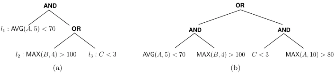
Two example query trees are shown in Figure 1, as-suming streams named A, B, and C, which are assumed to produce integer data items. Each leaf corresponds to a boolean predicate. A predicate may involve no operator, e.g., “C < 3” is true if the last item from stream C is strictly lower than 3, or based on an arbitrary operator (in this example MAX or AVG) which is applied to a time-window for a stream, e.g., “AVG(A, 5) < 70” is true if the average of the last 5 items from A is strictly lower than 70).
The problem of computing the truth value of a boolean query tree while incurring the minimum cost is known as Probabilistic AND-OR Tree Resolution (PAOTR) and has been studied extensively in the literature. In par-ticular, [6] provides both a survey of known theoretical results and several new results, all assuming that each data stream occurs in at most one leaf of the query tree. This assumption is termed read-once therein. In this case, for AND-trees (i.e., single-level trees with an AND operator at the root node) a simple O(n log n) greedy
OR AND l3: C < 3 l1: AVG(A, 5) < 70 l2: MAX(B, 4) > 100 (a) AND AND OR
AVG(A, 5) < 70 MAX(B, 4) > 100 C < 3 MAX(A, 10) > 80 (b)
Figure 1. Two query tree examples: (a) a read-once query; (b) a shared query.
algorithm produces an optimal leaf evaluation order (n is the number of leaves in the query tree) [7]. For DNF trees (i.e., collections of AND-trees whose roots are the children of a single OR node), a O(n log n) depth-first traversal of the trees that reuses the algorithm in [7] to order leaves within each AND produces an optimal evaluation order [6]. For general AND-OR-trees the complexity of the problem is open. The example query tree in Figure 1(a) is a read-once query since no stream occurs in two leaves.
By contrast, in this work we study the more general case, which we term shared, in which a stream can occur in multiple leaves. The example in Figure 1(b) corresponds to a shared case since stream A occurs in two leaves. Such queries are fairly common in, among others, telehealth scenarios. For example, an alert may be generated either if the heart rate is high (e.g., > 100) and the accelerometer is stationary or if the heart rate is low and SPO2 (blood oxygen saturation) is low. It is thus not difficult to imagine sensor streams appearing in multiple leaf predicates. The device that processes the query acquires data items from streams and holds each data item in memory until that data item is no longer relevant. A data item from a stream is no longer relevant when it is older than the maximum time-window used for that stream in the query. Each time a leaf of the query must be evaluated, one can then compute the number of data items that must be retrieved from the relevant stream given the time-windows of the operator applied to that stream and the data items from that stream that are already in the device’s memory. For example, considering the query in Figure 1(b), assume the predicate “AVG(A, 5) < 70” is evaluated first, thus pulling 5 items from stream A. If later the predicate “MAX(A, 10) > 80” needs to be evaluated then only 5 additional items must be pulled.
The shared scenario is important in practice, and has been introduced and investigated in [4]. In that work the authors do not give theoretical results, but instead develop heuristics to determine an order of operator evaluation that hopefully leads to low data acquisition costs. To the best of our knowledge, the complexity of the PAOTR problem in the shared case has never been addressed in the literature, likely because re-using
stream data across leaves dramatically complicates the problem. When picking a leaf evaluation order, inter-dependences between the leaves must be taken into account. In fact, even when given a leaf evaluation order, computing the expected query cost is intricate while this same computation is trivial in the read-once case.
In this work we study the PAOTR problem in the
shared case and make the following contributions: • For AND-trees we give an optimal algorithm (which
is much more involved than the optimal algorithm in the read-once case);
• For DNF trees we show that the problem is
NP-complete; but we are able to prove that there exists an optimal leaf evaluation order that is depth-first;
• For DNF trees we develop heuristics that we
eval-uate in simulation and compare to the optimal solution (computed via an exhaustive search) and to the heuristic proposed in [4].
In Section II we discuss models, the problem state-ment, and related work. We study AND-trees and DNF trees in Section III and Section IV, respectively. Sec-tion V concludes the paper with a brief summary of our findings and perspectives on future work. Detailed proofs of some of our theoretical results are provided in a technical report [8].
II. Problem Statement and Examples To define our problem we reuse the formalism and terminology in [6]. A query is an AND-OR tree, i.e., a rooted tree whose non-leaf nodes are AND or OR opera-tors, and whose leaf nodes are labeled with probabilistic boolean predicates. Each predicate is evaluated over data items generated by a data stream. The evaluation of each predicate has a known success probability (the probability that the predicate evaluates to TRUE) and a cost. In practice, the success probability can be esti-mated based on historical traces obtained from previous query evaluations. As in [6], we assume independent predicates, meaning that two predicates at two leaf nodes in a query are statistically independent. The cost is determined by the number of data items required to perform the evaluation and the evaluation cost per data item for the stream. For instance, the cost of a data item could correspond to the energy cost, in joules, of
acquiring one data item based on the communication medium used for the stream and the data item size.
More formally, we consider a set of s streams, S = {S1, . . . , Ss}. Stream Sk has a cost per data item of
c(Sk). A query on these streams, T , is a rooted
AND-OR tree with m leaves, l1, . . . , lm. Leaf lj has success,
resp. failure, probability pj, resp. qj = 1 − pj, and
requires the last dj items from stream S(j) ∈ S. The
objective is to compute the truth value of the root of the query tree by evaluating the leaves of the tree. Because each non-leaf node in a query tree is either an OR or an AND operator, it may not be necessary to evaluate all the leaves due to shortcircuiting. In other words, as soon as any child node of an OR, resp. AND, operator evaluates to TRUE, resp. FALSE, the truth value of the operator is known and can be propagated toward the root. For a given query, we define a schedule as an evaluation order of the leaves of the query tree, represented as a sorted sequence of the leaves.
We define the cost of a schedule as the expected
value of the sum of the costs incurred for all leaves that
are evaluated before the root’s truth value is determined. For instance, consider the query in Figure 1(a), in which leaves are labeled l1, l2, l3, and consider the schedule l2, l3, l1. The query processing begins with the
acquisi-tion of the data items necessary for evaluating l2, which
has cost 4 · c(B). With probability p2, l2 evaluates to
TRUE, thus shortcircuiting the evaluation of l3.
There-fore, the expected evaluation cost of the OR operator is: 4 · c(B) + q2 · c(C). If the OR operator evaluates
to FALSE, which happens with probability q2q3, then
the evaluation of l1is shortcircuited. Otherwise, l1must
be evaluated. The overall cost of the schedule is thus: 4 · c(B) + q2· c(C) + (1 − q2q3) · 5 · c(A). Recall that this
query tree is for a read-once scenario.
The PAOTR problem consists in determining a sched-ule with minimum cost. The complexity of this problem is unknown in the read-once case for general AND-OR trees, while optimal polynomial-time algorithms are known for AND-trees [7] and DNF trees [6]. In this work, we focus on these two types of trees in the shared case, seeking to develop optimal algorithms or to show NP-completeness. We refer the reader to [6] for a detailed review of the PAOTR literature. To the best of our knowledge, the only work that has studied the shared case is [4], in which a heuristic is proposed for DNF trees. We evaluate this heuristic in Section IV-D. In the next two sections we give examples of cost computations for an AND-tree and a DNF tree both in the shared case.
A. AND-tree example
Consider the AND-tree query depicted in Figure 2 with three leaves labeled l1, l2, and l3, for two streams A
and B. For each leaf (li), we indicate the stream (S(i)),
the number of data items needed from that stream to evaluate the leaf (di), and the success probability (pi).
For instance, leaf l2 requires d2 = 2 items from stream S(2) = A and evaluates to TRUE with probability p2 = 0.1. We assume that retrieving a data item from
a stream has unitary cost, regardless of the stream. There are 6 possible schedules for this tree, each schedule corresponding to one of the 3! orderings of the leaves. The optimal algorithm for read-once AND-trees sorts the leaves by non-decreasing djc(S(j))/qj [7]. Because
1×c(A) q1 = 1 1−0.75 = 4, 2×c(A) q2 = 2 1−0.1 ≈ 2.22, and 1×c(B) q3 = 1
1−0.5 = 2, this algorithm schedules leaf l3first.
There are two possible schedules with l3as the first leaf: • l3, l1, l2whose cost is: c(B)+p3×(c(A)+p1×c(A)) =
1 + 0.5 × (1 + 0.75 × 1) = 1.875; and
• l3, l2, l1 whose cost is: c(B) + p3× (2 × c(A) + p2×
0 × c(A)) = 1 + 0.5 × (2 + 0.1 × 0) = 2.
However, another schedule, l1, l2, l3, has a lower cost: c(A) + p1× (c(A) + p2× c(B)) = 1 + 0.75 × (1 + 0.1 × 1) =
1.825. Therefore, the optimal algorithm for the PAOTR problem for read-once AND-trees is no longer optimal in the shared case.
B. DNF tree example
Figure 3 shows a DNF tree with three AND nodes, for four streams A, B, C, and D. Each leaf requires only one data item from a stream. Leaves are labeled l1to l7,
in the order in which they appear in a given schedule. This example is meant to illustrate the difficulty of the PAOTR problem in the case of DNF trees in the shared scenario. In particular, computing the cost of a schedule is much more complicated than in the read-once scenario due to inter-leaf dependencies. Let Cj be the cost of
evaluating leaf lj, and C the overall cost of the schedule.
We consider the 7 leaves one by one, in order:
Leaf l1 – The first leaf is evaluated: C1= c(A).
Leaf l2 – This is the first leaf in its AND, no AND
has been fully evaluated so far, and l2 is the first
encountered leaf that requires stream B. Therefore, l2
is always evaluated, requiring a data item from stream
B: C2= c(B).
Leaf l3 – This is the second leaf from its AND, no
AND has been fully evaluated so far, and l3 is the first
and A[1] 0.75 l1 A[2] 0.1 l2 B[1] 0.5 l3
or
and1 and2 and3
A[1] l1 C[1] l3 D[1] l4 B[1] l2 C[1] l5 B[1] l6 D[1] l7
Figure 3. Example DNF tree.
encountered leaf that requires stream C. Therefore, a data item from C is acquired if and only if l1 evaluates
to TRUE: C3= p1c(C).
Leaf l4 – This is the third leaf from its AND, no
AND has been fully evaluated so far, and l4 is the first
encountered leaf that requires stream D. Therefore, one data item is acquired from D if and only if l1and l3both
evaluate to TRUE: C4= p1p3c(D).
Leaf l5 – This is the second leaf from its AND, and
AND1 has been fully evaluated so far. However, one of
the leaves of that AND, l3, requires a data item that
is also needed by l5, from stream C. If l3 has been
evaluated, then the evaluation cost of l5is 0 because the
necessary data item from C has already been acquired and is available “for free” when evaluating l5. If l3
has not been evaluated (with probability 1 − p1), it
means that AND1 has evaluated to FALSE. Then,
if l2 has evaluated to TRUE, l5 must be evaluated
thus requiring the data item from stream C. We obtain C5= (1 − p1)p2c(C).
Leaf l6 – Since l2 is always evaluated the data item
from stream B required by l6is always available for free:
C6= 0.
Leaf l7 – This is the second leaf from its AND, and
AND1 and AND2 have been fully evaluated so far.
However, one of the leaves of AND1, l4, but none of
those of AND2, require the data item that is needed
by l7 from stream D. Therefore, l7 must be evaluated
and its evaluation is not free if and only if l4 has not
been evaluated, AND2 has evaluated to FALSE, and
the evaluation of AND3 went as far as l7. Therefore,
C7= (1 − p1p3)(1 − p2p5)p6c(D).
Overall, we obtain the cost of the schedule: T C = c(A) + c(B) + (p1+ (1 − p1)p2)c(C)
+ (p1p3+ (1 − p1p3)(1 − p2p5)p6)c(D)
Given the complexity of the above cost computation, one might expect the PAOTR problem to be NP-complete in the shared case (recall that it is polynomial in the
read-once case). We confirm this expectation in Section IV.
III. AND trees
In this section, we focus on AND-trees. We have seen in Section II-A that the simple greedy algorithm proposed in [7] in the read-once case is not optimal in the shared case. We propose an algorithm and we prove that it is optimal. This algorithm is still greedy but compares the ratios of cost to failure probability of all sequences of leaves that use the same stream, instead of only considering pair-wise leaf comparisons. We begin in Section III-A with a preliminary result on the optimal ordering of leaves that use the same stream.
A. Ordering same-stream leaves
In the example given in Section II-A, we considered two schedules that begin with leaf l3. In the first schedule
leaf l1precedes l2, while the converse is true in the second
schedule. Leaf l1 requires one data item from stream A, while leaf l2 requires two data items from the same
stream. Therefore the first schedule is always preferable to the second schedule: if we evaluate l1before l2and if l1evaluates to FALSE, then there is no need to retrieve
the second data item and the cost is lowered. A general result can be obtained:
Proposition 1. Consider an AND-tree and a leaf lithat
requires di data items from a stream S. In an optimal
schedule li is scheduled before any leaf lj that requires
dj > di data items from stream S.
Proof: This proposition is proven via a simple exchange argument [8].
B. Optimal schedule
Consider an AND-tree with m leaves, l1, . . . , lm, for
s streams, S1, . . . , Ss. We define Lk = {lj|S(lj) = Sk},
i.e., the set of leaves that require data items from stream
Sk. Algorithm 1 shows a greedy algorithm (implemented
recursively for clarity of presentation) that takes as input the Lk sets, an initially empty schedule ξ, and
an array of s integers, NItems, whose elements are all initially set to zero. This array is used to keep track, for each stream, of how many data items from that stream have been retrieved in the schedule so far. Each call to the algorithm appends to the schedule a sequence of leaves that require data items from the same stream, in increasing order of number of data items required. The algorithm stops when all leaves have been scheduled. The algorithm first loops through all the streams (the k loop). For each stream, the algorithm then loops over all the leaves that use that stream, taken in increasing order of the number of items required. For each such leaf the algorithm computes the ratio (variable Ratio) of cost to probability of failure of the sequence of leaves up to that leaf. The leaf with minimum such ratio is selected (leaf lj0 in the algorithm, which requires dj0 data items
from stream S(lj0)). In the last loop of the algorithm,
all unscheduled leaves that require dj0 or fewer data
items from stream S(lj0) are appended to the schedule
in increasing order of the number of required data items.
Algorithm 1: GREEDY({L1, ..., Ls}, ξ, NItems)
if ∪s
i=1Li= ∅ then return ξ
M inRatio ← +∞
for k = 1 to s do loop on streams
Cost ← 0 P roba ← 1
N um ← NItems[k]
for lj in Lk by increasing dj do
Cost ← Cost + P roba × (dj− N um) × c(k)
P roba ← P roba × pj
N um ← dj
Ratio ← (1−P roba)Cost
if Ratio < M inRatio then
M inRatio ← Ratio j0← j for lj in LS(j0) by increasing dj do if dj≤ dj0 then ξ.append(lj) LS(j0)← LS(j0)\ {lj} NItems[S(j0)] ← dj0
return GREEDY ({L1, ..., Ls}, ξ, NItems)
Theorem 1. Algorithm 1 is optimal for the shared
PAOTR problem for AND-trees.
Proof Sketch: We prove the theorem by contra-diction. We assume that there exists an instance for which the schedule produced by Algorithm 1, ξgreedy,
is not optimal. Among the optimal schedules, we pick a schedule, ξopt, which has the longest prefix P in common
with ξgreedy. We consider the first decision taken by
Algorithm 1 that schedules a leaf that does not belong to P. Let us denote by lσ(1), ..., lσ(k) the sequence of
leaves scheduled by this decision. The first leaves in this sequence may belong to P. Let P0 be P minus the leaves
lσ(1), ..., lσ(k). Then, ξgreedy can be written as:
ξgreedy= P0, lσ(1), ..., lσ(k), S.
In turn, ξopt can be written ξopt = P0, Q, R where lσ(k)
is the last leaf of Q. In other words, Q can be written
L1, lσ(1), ..., Lk, lσ(k), where each sequence of leaves Li,
1 ≤ i ≤ k, may be empty. We can write:
ξopt= P0, L1, lσ(1), ..., Lk, lσ(k), R.
From ξgreedy and ξopt, we build a new schedule, ξnew,
defined as
ξnew= P0, lσ(1), ..., lσ(k), L1, ..., Lk, R.
P0, lσ(1), ..., lσ(k)is a prefix to both ξgreedyand ξnew. This
prefix is strictly larger than P since P does not contain
lσ(k). We compute the cost of ξnew and show that it is
no larger than that of ξopt, thus showing that ξnew is
optimal and has a longer prefix in common with ξgreedy
than ξnew, which is a contradiction. This computation is
very lengthy and technical and the full proof is provided in [8].
The complexity of Algorithm 1 is O(m2). Indeed, the sets L1, ..., Ls are built and sorted in O(m log(m))
and there are at most m recursive calls to Algorithm 1, each having a cost proportional to the number of leaves remaining in the AND tree.
One may wonder how the optimal algorithm in the
read-once case [7], which simply sorts the leaves by
increasing djc(S(j))/qj, fares in the shared case. In other
terms, is Algorithm 1 really needed in practice? Figure 4 shows results for a set of randomly generated AND-trees. We define the sharing ratio, ρ, of a tree as the expected number of leaves that use the same stream, i.e., the total number of leaves divided by the number of streams. For a given number of leaves m = 2, . . . , 20 and a given sharing ratio ρ = 1, 5/4, 4/3, 3/2, 2, 3, 4, 5, 10, we generate 1,000 random trees for a total of 157,000 random trees (note that ρ cannot be larger than the number of leaves). Leaf success probabilities, numbers of data items needed at each leaf, and per data item costs are sampled from uniform distributions over the intervals [0, 1], [1, 5], and [1, 10], respectively. For each tree we compute the cost achieved by the algorithm in [7] and that achieved by our optimal algorithm. Figure 4 plots these costs for all instances, sorted by increasing optimal cost. Due to this sorting, the large number of samples, and the limited resolution, the set of points for the optimal algorithm appears as a curve while the set of points for the algorithm in [7] appears as a cloud of points. The algorithm in [7] can lead to costs up to 1.86 times larger than the optimal. It leads to costs more than 10% larger for 19.54% of the instances, and more than 1% larger for 60.20% of the instances. The two algorithms lead to the same cost for 11.29% of the instances. We conclude that, in the shared case, Algorithm 1 provides substantial improvements over the optimal algorithm for the read-once case.
IV. DNF Trees
In this section we consider DNF trees. First, in Section IV-A we provide a method for computing the expected cost of a given schedule for a DNF tree. In Section IV-B we show that depth-first schedules
40000 Cost 60 40 20 0
Shared instances sorted by increasing optimal cost 120000 80000
0
Algorithm in [7] Optimal algorithm
Figure 4. Cost achieved by the algorithm in [7] and that achieved by the optimal algorithm, shown for each of the 157,000 AND-tree instances sorted by increasing optimal cost.
are dominant, which means that there always exists a depth-first schedule that is optimal. In Section IV-C, we then prove that the problem is NP-complete. This is in sharp contrast with the read-once case, in which a simple greedy algorithm is optimal [6]. In Section IV-D we propose several heuristics to schedule a DNF tree and evaluate their performance on randomly generated problem instances.
A. Evaluation of a schedule
We have seen in Section II-B in an example that computing the cost of a schedule is non-trivial for DNF trees. In this section we formalize this computation. Consider a DNF tree with N AND nodes, indexed
i = 1, . . . , N . AND node i has mi leaves, denoted by
li,j, j = 1, . . . , mi. The probability of success of leaf li,j
is denoted by pi,j, and the stream that leaf li,jrequires is
denoted by S(i, j). We use L to denote the set of all the leaves. We consider a schedule ξ, which is an ordering of the leaves, and use ls,t≺ lu,v to indicate that leaf ls,t
occurs before leaf lu,v in ξ. We consider that the query
is over s streams, Sk, k = 1, . . . , s. The cost per data
item of Sk is denoted by c(Sk). We define the “t-th data
item” of a stream as the data item produced t time-steps ago, so that the first data item is the one produced most recently, the second is the one produced before the first, etc. In this manner, when we say that a leaf li,jrequires
di,j data items it means that it requires all t-th data
items of the stream for t = 1, 2, . . . , di,j.
Given the above, we define Lk,tas the set of the leaves
that require the t-th data item from stream Sk, and that
are the first of their respective AND nodes to require that data item. Formally, we have:
Lk,t= li,j∈ L
S(i, j) = Sk, di,j≥ t, and
∀r 6= j, S(i, r) 6= Sk or di,r< t
or li,j≺ li,r
We also define Ai,j, the index set of all AND nodes that
have been fully evaluated before a leaf li,j is evaluated,
as:
Ai,j = {k | mk= |{lk,r|lk,r≺ li,j}|}.
If we use Ci,j,t to denote the expected cost of retrieving
the t-th data item of the relevant stream when evaluating leaf li,j, then the total cost C of the schedule ξ is:
C = N X i=1 mi X j=1 di,j X t=1 Ci,j,t.
The following proposition gives Ci,j,t.
Proposition 2. Given a leaf li,j that requires the t-th
data item from stream Sk, if there exists r such that li,r≺
li,j and li,r∈ Lk,t, then Ci,j,t= 0. Otherwise:
Ci,j,t= Y lr,s∈Lk,t lr,s≺li,j 1 − Y lr,u≺lr,s pr,u × Y a∈Ai,j 6∃r, la,r∈Lk,t 1 − ma Y r=1 pa,r ! × Y li,u≺li,j pi,u × c(S(i, j)).
Proof: Consider a schedule ξ, and a leaf in that
schedule, li,j, which requires the t-th data item from
stream Sk (i.e., S(i, j) = Sk). Let us prove the first
part of the proposition. If a leaf li,r (i.e., a leaf under
the same AND node as li,j) occurs before li,j in ξ and
requires the t-th item from stream Sk (i.e., li,r ∈ Lk,t),
then there are two possibilities. Either li,r has been
evaluated, in which case the evaluation of li,juses a data
item that has already been acquired previously, hence a cost of 0. Or li,k has not been evaluated, meaning that
its evaluation was shortcircuited. In this case the AND node has evaluated to FALSE and the evaluation of li,j
is also shortcircuited, hence a cost of 0.
The second part of the proposition shows the expected cost as a product of three factors, each of which is a probability, and a fourth factor, c(S(i, j)), which is the cost of acquiring the data item from the stream. The interpretation of the expression for Ci,j,t is as follows: a
leaf must acquire the item if and only if (i) the item has not been previously acquired; and (ii) no AND node has already evaluated to TRUE; and (iii) no leaf in the same AND node has already evaluated to FALSE. We explain the computation of these three probabilities hereafter.
The first factor is the probability that none of the leaves that precede li,j in ξ and that require the t-th
item from stream Sk have been evaluated. Such a leaf
that precede it in the schedule have evaluated to TRUE, which happens with probability Q
lr,u≺lr,spr,u. Hence,
the expression for the first factor.
The second factor is the probability that none of the AND nodes that have been fully evaluated so far has evaluated to TRUE, since if this were the case the evaluation of li,j would not be needed, leading to a
cost of 0. Given an AND node in Ai,j, say the k-th
AND node, the probability that it has been evaluated to TRUE isQmk
r=1pk,r. This is true except if one of the
leaves of that AND node belongs to Lk,t. The first factor
assumes that that leaf was not evaluated and, therefore, that that entire AND node was not evaluated. Hence, the expression for the second factor.
The third factor is the probability that all the leaves in the same AND as li,jhave evaluated to TRUE. Because
we are in the second case of the proposition, none of these leaves requires the t-th item of stream Sk. All these
leaves must evaluate to TRUE, otherwise the evaluation of li,jwould be shortcircuited, for a cost of 0. Hence, the
expression for the third factor.
Cost of the evaluation of a schedule: To compute this
cost, we need to introduce two new notations. Let |L| be the total number of leaves in the considered DNF, and let D be the maximum number of data items required by a stream. Then, we have |L| = PN
i=1mi and D =
max1≤iN,1≤j≤midi,j.
To compute all the sets Lk,twe need to scan the leaves
of each AND node according to the schedule ξ while recording the maximum number of elements required from each stream. The overall cost of this scheme is
O(|L|). Each set Lk,t contains at most N leaves.
Computing all the sets Ai,j is also done through
a traversal of the set of leaves, for an overall cost of O(|L| + N2) (because the sets Ai,j take at most
N − 1 distinct values and each contains at most N − 1
elements). Computing all the product of probabilities used in the computation of all the Ci,j,tcan also be done
in a single traversal of the set of leaves.
Once all these precomputations are done, the first term in the expression of Ci,j,tcan be computed in O(N )
and the second in O(N2), and the third one in O(1). Overall the cost of a schedule can be evaluated with complexity
O(|L|DN2).
B. Dominance of depth-first schedules
Theorem 2. Given a DNF tree, there exists an optimal
schedule that is depth-first, i.e., that processes AND nodes one by one.
Proof: Consider a DNF tree T and a schedule ξ.
Without loss of generality we assume that the AND nodes, A1, . . . , An, are numbered in the order of their
completion. Thus, according to ξ, A1 is the first AND
node with all its leaves evaluated. We denote by M the number (possibly zero) of AND nodes that ξ processes one by one and entirely at the start of its execution. Therefore, if ξ evaluates a leaf li,j, with i 6= 1, in the
m1first steps, then M = 0. Finally, we assume that the
leaves of an AND node are numbered according to their evaluation order in ξ.
We prove the theorem by contradiction. Let us assume that there does not exist a schedule that satisfies the desired property. Let ξ be an optimal schedule that max-imizes M . By definition of M and by the hypothesis on the numbering of the AND nodes, schedule ξ evaluates some leaves of the AND nodes AM +2, ..., An before it
evaluates the last leaf of AM +1. Let L denote the set
of these leaves. We now define a new ξ0 which starts by executing at least M + 1 AND nodes one by one:
• ξ0 starts by evaluating the first M AND nodes one
by one, evaluating their leaves in the same order and at the same steps as in ξ;
• ξ0then evaluates all the leaves of AM +1in the same
order as in ξ (but not at the same steps);
• ξ0 then evaluates the leaves in L in the same order
as in ξ (but not at the same steps);
• ξ0finally evaluates the remaining leaves in the same order and at the same steps as in ξ.
The cost of a schedule is the sum, over all potentially acquired data items, of the cost of acquiring each data item times the probability of acquiring it. Let d be a data item potentially needed by a leaf in T . We show that the probability of acquiring d is not greater with ξ0 than with ξ. We have three cases to consider.
Case 1) d is not needed by a leaf of AM +1 and not
needed by a leaf in L. Then d’s probability to be acquired is the same with ξ and ξ0.
Case 2) d is needed by at least one leaf of AM +1.
The only way in which a leaf that is evaluated in ξ would not be evaluated in ξ0 is if AM +1 evaluates to
TRUE. By assumption, however, at least one leaf of
AM +1uses d. Therefore, for AM +1to evaluate to TRUE,
d must be acquired. Consequently, the probability that d is acquired is the same with ξ and with ξ0.
Case 3) d is needed by at least one leaf in L but not
needed by any leaf of AM +1. ξ and ξ0 define the same
ordering on the leaves in L. For each AND node Ai, with
M + 2 ≤ i ≤ N , there is at most one leaf in Ai∩ L that
can be the leaf responsible for the acquisition of d with
ξ, and it is the same leaf with ξ0. Let F be the set of all
these leaves. Then, with ξ, the leaves in F are responsible for the acquisition of d if and only if:
• A1, ..., AM all evaluate to FALSE;
• None of the evaluated leaves of A1, ..., AM needs d;
and
Let us denote by P the probability that all the AND nodes A1, ..., AM evaluate to FALSE and that none
of the evaluated leaves of these AND nodes needs the data item d. Let us denote by D the probability that d is acquired because of the evaluation of one of the leaves of the AND nodes A1, ..., AM. Finally, let R be the
probability that one of the leaves evaluated with ξ after
lM +1,mM +1 acquires d, knowing that no leaves of A1, ...,
AM or in L acquires it. Then, with ξ, the probability p
that d is acquired is:
p = D + P 1 − Y li,j∈F 1 − j−1 Y k=1 pi,k ! + R (1)
because leaf li,j is evaluated with probability Q j−1 k=1pi,k,
that is, if all the leaves from the same AND node that are evaluated prior to it all evaluate to TRUE. The second term of Equation (1) is the probability that the leaves in F are responsible for acquiring d.
With schedule ξ0, the leaves of F are responsible for the acquisition of d if and only if:
• The AND nodes A1, ..., AM, and AM +1all evaluate
to FALSE;
• None of the evaluated leaves of the AND nodes A1,
..., AM need d; and
• At least one of the leaves in F is evaluated. Thus, with ξ0, the probability p0 that d is acquired is:
p0 = D + P 1 − mM +1 Y k=1 pM +1,k ! × 1 − Y li,j∈F 1 − j−1 Y k=1 pi,k ! + R Comparing this equation with Equation 1, we see that
p0 is not greater than p.
The probability that a data item is acquired with ξ0is thus not greater than with ξ. Therefore, in each of the three cases the cost of ξ0 is not greater than the cost of ξ, meaning that ξ0 is also an optimal schedule. Since
ξ0 starts by executing at least M + 1 AND nodes one
by one, we obtain a contradiction with the maximality assumption on M , which concludes the proof.
C. NP-completeness
In the read-once case, an optimal algorithm for DNF trees is built on top of the optimal algorithm for AND-trees [6]. The same approach cannot be used in the
shared case, as seen in a simple counter-example [8]. In
other words, for some DNF trees, the ordering of the leaves of a given AND node in an optimal schedule does not correspond to the ordering produced by Algorithm 1 for that AND node. And, in fact, in this section we show
the NP-completeness of finding an optimal schedule to evaluate a DNF tree.
Definition 1 (DNF-Decision). Given a DNF tree and
a cost bound K, is there a schedule whose expected cost does not exceed K?
Theorem 3. DNF-Decision is NP-complete.
Proof: The NP-completeness is obtained via a
non-trivial reduction from 2-PARTITION [9]. See [8] for the proof.
D. Heuristics
Given the NP-completeness result in the previous sec-tion, we now propose several polynomial-time heuristics for computing a schedule. These heuristics fall into three categories, which we term leaf-ordered, AND-ordered, and stream-ordered.
Leaf-ordered heuristics simply sort the leaves
accord-ing to leaf costs (C), failure probabilities (q = 1 − p), or the ratio of the two, which leads to three heuristics plus a baseline random one:
• Leaf-ordered, decreasing q (prioritizes leaves with
high chances of shortcutting the evaluation of an AND node);
• Leaf-ordered, increasing C (prioritizes leaves with
low costs);
• Leaf-ordered, increasing C/q (prioritizes leaves with
low costs and also with high chances of shortcutting the evaluation of an AND node);
• Leaf-ordered, random (baseline).
The above first three heuristics have intuitive rationales. Other options are possible (e.g., sort leaves by decreasing C) but are easily shown to produce poor results.
AND-ordered heuristics, unlike leaf-ordered
heuris-tics, account for the structure of the DNF tree by build-ing depth-first schedules, with the rationale that there is a depth-first schedule that is optimal (Theorem 2). Furthermore, Algorithm 1 provides a way to compute an optimal schedule for the leaves within the same AND node. For this optimal schedule one can compute the (expected) cost and the probability of success of the AND node using the method in Section IV-A. Therefore, AND-ordered heuristics simply order the AND nodes based on their computed costs (C), computed probability of success (p), or ratio of the two, and using Algorithm 1 for scheduling the leaves of each AND node, leading to three heuristics:
• AND-ordered, decreasing p (prioritizes AND’s with
high chances of shortcircuiting the evaluation of the OR node);
• AND-ordered, increasing C (prioritizes AND’s with
• AND-ordered, increasing C/p (prioritizes AND’s
with low costs and also with high chances of short-circuiting the evaluation of the OR node);
There are two approaches to compute the cost of an AND node: (i) consider the AND node in isolation assuming that the OR node has a single AND node child; or (ii) account for previously scheduled AND nodes whose evaluation has caused some data items to be acquired with some probabilities. We terms the first approach “static” and the second approach “dynamic,” giving us two versions of the last two heuristics above.
Stream-ordered heuristics proceed by ordering the
streams from which data items are acquired, acquiring all items from a stream before proceeding to the next stream, until the truth value of the OR node has been determined. This idea was proposed in [4], and to the best of our knowledge it is the only previously proposed heuristic for solving the PAOTR problem in the shared scenario for DNF trees. For each stream S the heuristic computes a metric, R(S), defined as follows:
R(S) =
P
i,j|S(i,j)=Sqi,jni,j
maxi,j|S(i,j)=Sdi,jc(S)
,
where ni,j is the number of leaf nodes whose evaluation
would be shortcircuited if leaf li,j was to evaluate to
FALSE. The numerator can thus be interpreted as the shortcutting power of stream S. The denominator is the maximum data element acquisition cost over all the leaves that use stream S. The heuristic orders the streams by increasing R values. The rationale is that one should prioritize streams that can shortcut many leaf evaluations and that have low maximum data item acquisition costs. The heuristic as it is described in [4] acquires the maximum number of needed data items from each stream so as to compute truth values of all the leaves that require data items from that stream. In other words, the leaves that require data items from the same stream are scheduled in decreasing di,j order. However,
Proposition 1 holds for DNF trees, showing that it is always better to schedule these leaves in increasing di,j
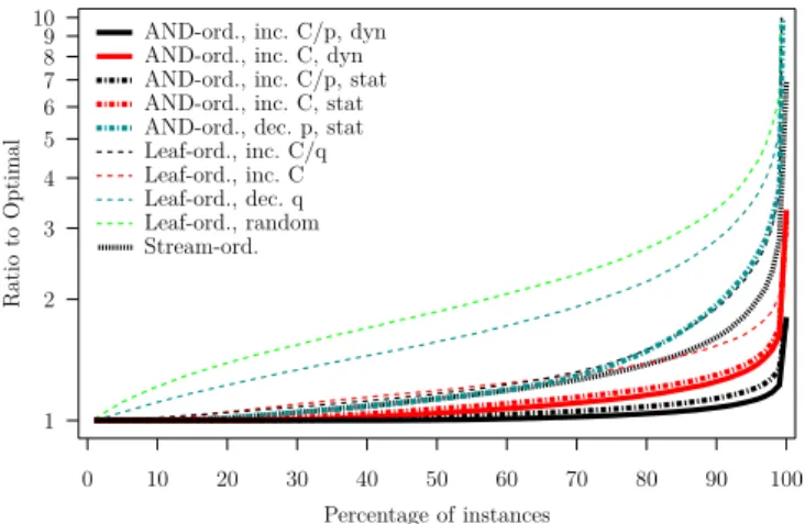
order. We use this leaf order to implement this heuristic in this work. We have verified in our experiments that this version outperforms the version in [4] in the vast majority of the cases, with all remaining cases being ties. In total, we consider 4 leaf-ordered, 5 AND-ordered, and 1 stream-ordered heuristics. We first evaluate these heuristics on a set of “small” instances for which we can compute optimal schedules using an exponential-time algorithm that performs an exhaustive search. Such an algorithm is feasible because, due to Theorem 2, it only needs to search over all possible depth-first schedules. Small instances are generated using the same method as that described in Section III-B for generating AND-tree instances. We generate DNF
Ratio to Optimal 0 10 20 30 40 50 60 70 80 90 100 Percentage of instances 1 2 3 4 5 6 7 8 9 10 Stream-ord. Leaf-ord., random Leaf-ord., dec. q Leaf-ord., inc. C Leaf-ord., inc. C/q AND-ord., dec. p, stat AND-ord., inc. C, stat AND-ord., inc. C/p, stat AND-ord., inc. C, dyn AND-ord., inc. C/p, dyn
Figure 5. Ratio to optimal vs. fraction of the instances for which a smaller ratio is achieved, computed over the 21,600 “small” DNF tree instances.
trees with N = 2, . . . , 9 AND nodes and up to at most 20 leaves and 8 leaves per AND, generating 100 random instances for each configuration, for a total of 21,600 instances (The source code is available at www.ens-lyon.fr/LIP/ROMA/Data/DataForRR-8373.tgz). For each instance we compute the ratio between the cost achieved by each heuristic and the optimal cost. Figure 5 shows for each heuristic the ratio vs. the fraction of the instances for which the heuristic achieves a lower ratio. For instance, a point at (80, 2) means that the heuristic leads to schedules that are within a factor 2 of optimal for 80% of the instances, and more than a factor 2 away from optimal for 20% of the instances. The better the heuristic the closer its curve is to the horizontal axis.
The trends in Figure 5 are clear. Overall the poorest results are achieved by the leaf-ordered heuristics, with the random such heuristic expectedly being the worst and the increasing C the best. The AND-ordered heuris-tics, save for the decreasing p version, lead to the best re-sults overall. More precisely, the best rere-sults are achieved by sorting AND’s by increasing C/p, with sorting by increasing C leading to the second-best results. For the two AND-ordered heuristics that have both a static and a dynamic version, the dynamic version leads to marginally better results than the static version. Finally, the stream-ordered heuristic leads to poorer results than the best leaf-ordered heuristics, and thus significantly worse than the best AND-ordered heuristics.
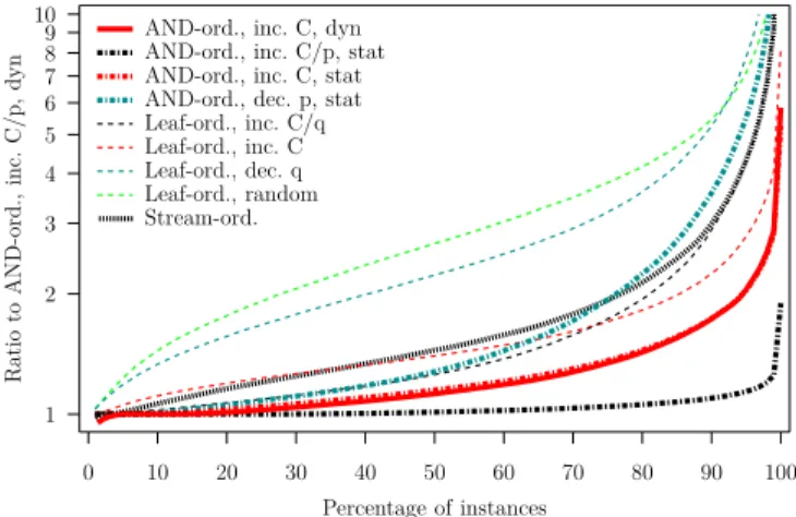
We also evaluate the heuristics on a set of “large” instances with N = 2, . . . , 10 AND nodes and m = 5, 10, 15, 20 leaves per AND node, with 100 random instances per configuration, for a total of 32,400 in-stances. For most of these instances we cannot tractably compute the optimal cost. Consequently, we compute ratios to the cost achieved by the AND-ordered by increasing C/p dynamic heuristic, which leads to the best
Ratio to AND-ord., inc. C/p, dyn 0 10 20 30 40 50 60 70 80 90 100 Percentage of instances 1 2 3 4 5 6 7 8 9 10 Stream-ord. Leaf-ord., random Leaf-ord., dec. q Leaf-ord., inc. C Leaf-ord., inc. C/q AND-ord., dec. p, stat AND-ord., inc. C, stat AND-ord., inc. C/p, stat AND-ord., inc. C, dyn
Figure 6. Ratio to AND-ordered increasing C/p dynamic vs. fraction of the instances for which a smaller ratio is achieved, computed over the 32,400 “large” DNF tree instances.
results for small instances. Results are shown in Figure 6. Essentially, all the observations made on the results for small instances still hold. We conclude that the best approach is to build a depth-first schedule, to sort the AND nodes by the ratio of their costs to probability of success, and to compute these costs dynamically, accounting for previously scheduled AND nodes. This heuristic is the best one in 94.5%, resp. 83.8%, of the cases reported in Figure 6, resp. Figure 5. It runs in less than 5 seconds on a 1.86 GHz core when processing a tree with 10 AND nodes with each 20 leaves.
V. Conclusion
Motivated by a query processing scenario for sensor data streams, we have studied a version of the Proba-bilistic And-Or Tree Resolution (PAOTR) problem [6] in which a data stream can be referenced by multiple leaves. We have given an optimal algorithm in the case of AND-trees and have shown NP-completeness in the case of DNF trees. For DNF we have shown that there is an optimal solution that corresponds to a depth-first traversal of the tree. This observation provides inspiration for a heuristic that largely outperforms the heuristic previously proposed in [4].
A possible future direction is to consider so-called
non-linear strategies [6]. Although in this work we have
con-sidered a schedule as a leaf ordering (called a linear
strat-egy in [6]), a more general notion is that of a decision tree
in which the next leaf to be evaluated is chosen based on the truth value of the previous evaluated leaf. A practical drawback of a non-linear strategy is that the size of the strategy’s description is exponential in the number of tree leaves. In [6], it is shown that in the read-once case linear strategies are dominant for DNF trees, meaning that there is always one optimal strategy that is linear. Via a simple counter example it can be shown that this is
no longer true in the shared case [8], thus motivating the investigation of non-linear strategies. Another possible future direction is to consider a less restricted version of the problem in which a single predicate at a leaf can access multiple streams rather than just a single one (e.g., “AV G(X, 10) < 10 ≥ M IN (Y, 20)”). There is no reason for real-world queries to be limited to a single stream per predicate. An interesting question, then, is whether the PAOTR problem remains polynomial for AND-trees or whether it becomes NP-complete.
Acknowledgments. Yves Robert is with Institut
Univer-sitaire de France. This work is supported by the INRIA associate team Aloha, and by the ANR project Rescue.
References
[1] E. Miluzzo, “Sensing Meets Mobile Social Networks: The Design, Implementation and Evaluation of the CenceMe Application,” in Proc. of ACM Conf. on Embedded Net-worked Sensor Systems, 2008.
[2] I. Mohomed, A. Misra, M. Ebling, and W. Jerome, “Context-Aware and Personalized Event Filtering for Low-Overhead Continuous Remote Health Monitoring,” in Proc. of the IEEE Intl. Symp. on a World of Wireless Mobile and Multimedia Networks, 2008.
[3] S. Gaonkar, J. Li, R. Roy Choudhury, L. Cox, and A. Schmidt, “Micro-Blog: Sharing and Querying Con-tent through Mobile Phones and Social Participation,” in Proc. of the ACM Intl. Conf. on Mobile Systems, Applications, and Services, 2008.
[4] L. Lim, A. Misra, and T. Mo, “Adaptive Data Acqui-sition Strategies for Energy-Efficient Smartphone-based Continuous Processing of Sensor Streams,” Distributed Parallel Databases, vol. 31, no. 2, pp. 321–351, 2013. [5] “The SHIMMER sensor platform,” http:
//shimmer-research.com, 2013.
[6] R. Greiner, R. Hayward, M. Jankowska, and M. Mol-loy, “Finding Optimal Satisficing Strategies for And-Or Trees,” Artificial Intelligence, vol. 170, no. 1, pp. 19–58, 2006.
[7] D. E. Smith, “Controlling backward inference,” Artificial Intelligence, vol. 39, no. 2, pp. 145––208, 1989.
[8] H. Casanova, L. Lim, Y. Robert, F. Vivien, and D. Zaidouni, “Cost-Optimal Execution of Trees of Boolean Operators with Shared Streams,” Inria, Research Report RR-8373, 2013, http://hal.inria.fr/hal-00869340. [9] M. R. Garey and D. S. Johnson, Computers and In-tractability, a Guide to the Theory of NP-Completeness. W.H. Freeman and Company, 1979.

![Figure 4. Cost achieved by the algorithm in [7] and that achieved by the optimal algorithm, shown for each of the 157,000 AND-tree instances sorted by increasing optimal cost.](https://thumb-eu.123doks.com/thumbv2/123doknet/14396200.509169/7.918.85.446.107.339/figure-achieved-algorithm-achieved-optimal-algorithm-instances-increasing.webp)