Comparative evaluation of cooling tower drift eliminator performance

(1)

COMPARATIVE EVALUATION OF COOLING TOWER DRIFT ELIMINATOR PERFORMANCE

by Joseph K. Chan and Michael W. Golay Energy Laboratory and

Department of Nuclear Engineering Massachusetts Institute of Technology

Cambridge, Massachusetts 02139

Final Report for Task #3 of the Waste Heat Management Research Program

110

110 111

(8)

4.6 Pressure Loss and Air Speed Measurement Techniques

4.7 Sources of Experimental Error Chapter 5.1 5.2 5.3 5.4 Chapter 6.1 6.2

5. Comparison of Experimental Results with Theoretical Calculations

Introduction

Pressure Drop Across Eliminators Collection Efficiency Results Estimation of Experimental Error

6. Conclusions and Recommendations Discussion of Results

Recommendat ions References

Appendix A DATANA Program A.1 Introduction

A.2 Description of the Programs A.3 Description of Input Parameters A.4 Listing of the DATANA Code

A.5 Sample Problem

132 134 139 139 141 144 150 153 153 172 179 186 186 186 191 195 223

(9)

Appendix B DAMIE Program 239

B.1 Introduction 239

B.2 Description of the Program 240

B.3 Description of the Input Parameters 241

B.4 Listing of the DAMIE Code 243

(10)

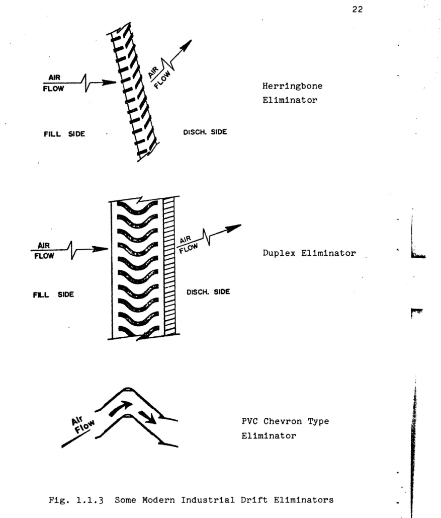
1.1.3 Some Modern Industrial Drift Eliminators 22 2.3.1 General Mesh Arrangement in SOLASUR.

Fictitious Boundary Cells are Shaded 47 2.3.2 Arrangement of Finite Difference Variables

in a Typical Cell 48

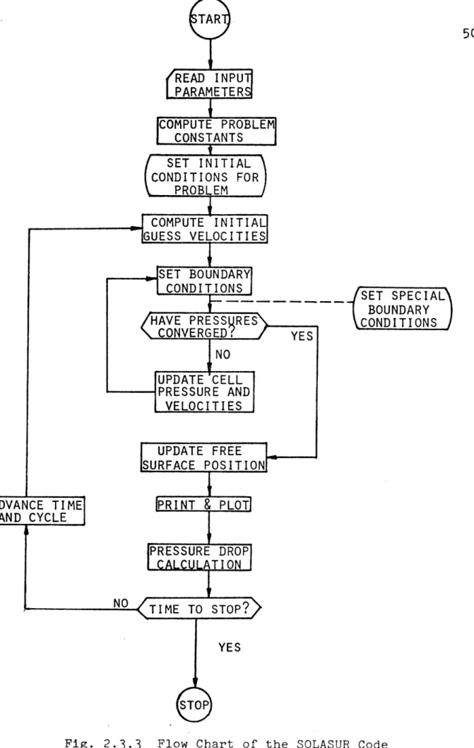
2.3.3 Flow Chart of the SOLASUR Code 50

2.5.1 Flow Chart of the DRIFT Code 58

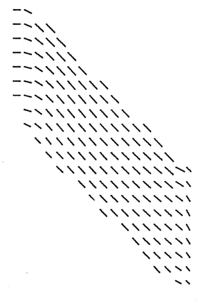
3.2.1 Velocity Distribution of Air Flow in Single-Layer Louver Eliminator Using Free-Slip

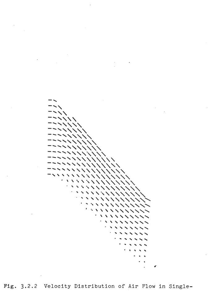
Conditions at Upper and Lower Boundaries 62 3.2.2 Velocity Distribution of Air Flow in

Single-Layer Louver Eliminator Using No-Slip

Double-Layer Louver Eliminator Using Free-Slip

Double-Layer Louver Eliminator Using No-Slip

Sinus-Shaped Eliminator. (A) Free-Slip Conditions at Upper and Lower Boundaries. (B) No-Slip

Conditions at Upper and Lower Boundaries 67 3.2.6 Velocity Distribution of Air Flow in Hi-V

Eliminator. (A) Free-Slip Conditions at Upper and Lower Boundaries. (B) No-Slip Conditions

(11)

9

No.

3.2.7 Velocity Distribution of Air Flow in Zig-Zag Eliminator Using Free-Slip Conditions

at Upper and Lower Boundaries 69

3.2.8 Velocity Distribution of Air Flow in Zig-Zag Eliminator Using No-Slip Conditions at

Upper and Lower Boundaries 70

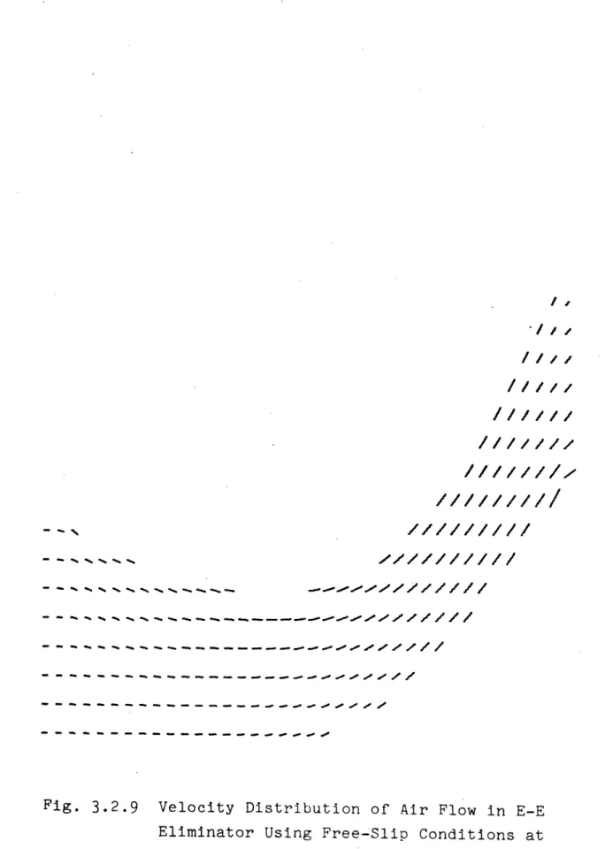
3.2.9 Velocity Distribution of Air Flow in E-E Eliminator Using Free-Slip Conditions at

3.2.10 Velocity Distribution of Air Flow in E-E Eliminator Using No-Slip Conditions at

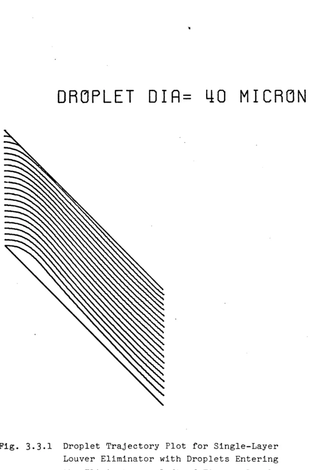
3.3.1 Droplet Trajectory Plot for Single-Layer Louver Eliminator with Droplets Entering the Eliminator at Left of Figure . Droplet

Size is 40 pm 77

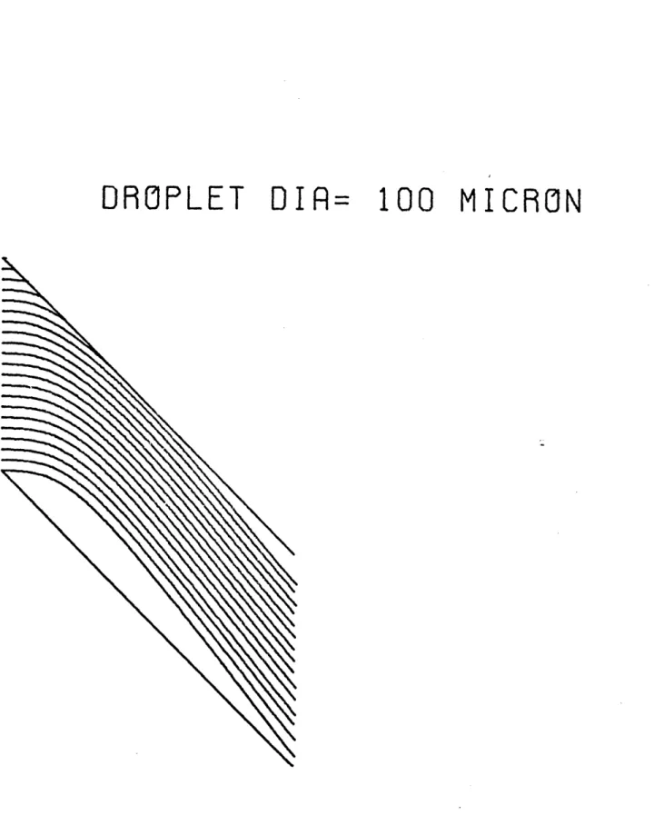
3.3.2 Droplet Trajectory Plot for Single-Layer Louver Eliminator with Droplets Entering the Eliminator at Left of Figure . Droplet

Size is 100 m 78

3.3.3 Droplet TrajectOry Plot for Double-Layer Louver Eliminator with Droplets Entering the Eliminator at Left of Figure . Droplet

Size is 40 um 80

3.3.4 Droplet Trajectory Plot for Double-Layer Louver Eliminator with Droplets Entering the Eliminator at Left of Figure . Droplet

Size is 100 m 81

3.3.5 Droplet Trajectory Plot for Sinus Shaped Eliminator with Droplets Entering the

Eliminator at the Left of Figure . Droplet

Size is 40 m 82

3.3.6 Droplet Trajectory Plot for Sinus Shaped Eliminator with Droplets Entering the

Eliminator at the Left of Figure . Droplet

Size is 100 m 83

(12)

3.3.8 Droplet Trajectory Plot for Asbestos-Cement Eliminator with Droplets

Entering the Eliminator at Left of Figure

Droplet Size is 100 pm 86

3.3.9 Droplet Trajectory Plot for Hi-V Elim-inator with Droplets Entering the Elimi-nator at Left of Figures.

(A) 40 pm Droplet Size

(B) 100 m Droplet Size 87

3.3.10 Droplet Trajectory Plot for Zig-Zag Eliminator with Droplets Entering the Eliminator at Left of Figure . Droplet

Size is 30 m 89

3.3.11 Droplet Trajectory Plot for Zig-Zag Eliminator with Droplets Entering the

Eliminator at Left of Figure . Droplet 90

Size is 60 m 90

3.3.12 Droplet Trajectory Plot for Two-Layer Zig-Zag Eliminator with Droplets Entering the Eliminator at Left of Figure . Droplet

Size is 30 m. 91

3.3.13 Droplet Trajectory Plot for Two-Layer Zig-Zag Eliminator with Droplets Entering the Eliminator at Left of Figure . Droplet

Size is 60 m 92

3.3.14 Droplet Trajectory Plot for E-E Elimi-nator with Droplets Entering the

Elimina-tor at Left of Figure . Droplet Size is

30 m 93

3.3.15 Droplet Trajectory Plot for E-E nator with Droplets Entering the Elimi-nator at Left of Figure . Droplet Size

(13)

11

No.

3.4.1 Collection Efficiency of Droplets as a Function of Droplet Size

(a) DRIFT Calculation

(b) Roffman Calculation 96

3.4.2 Collection Efficiency of Droplets as a Function of Droplet Size

(a) Sinus-Shaped Eliminator (b) Double-Layer Louver

Eliminator of Same Dimensions.

(Air Inlet Velocity=l m/s) 98 3.5.1 Pressure Drop Distribution Along the

Length of Sinus-Shaped Eliminator 102 3.5.2 Pressure Drop Distribution Along the

Length of Asbestos-Cement Eliminator 103 3.5.3 Pressure Drop Distribution Along the

Length of E-E Eliminator 104

3.5.4 Pressure Drop Distribution Along the

Length of Double-Layer Louver Eliminator 106 3.5.5 Pressure Drop Distribution Along the

Length of Hi-V Eliminator 107

4.2.1 Schematic Diagram of Drift Elimination

Facility 112

4.3.1 Schematic Diagram of Light Scattering

Drift Measurement Instrumentation 116 4.3.2 Scattered Light Intensity Versus Droplet

Size Calculated by DAMIE 117

4.4.1 Schematic Diagram of the Model 3050 Vibrating Orifice Monodisperse Aerosol

Generator 121

4.4.2 Schematic Diagram of the Droplet Generating

System 122

4.5.1 Intensity Distribution Across the Laser

(14)

4.5.3 Calibration Curve - the Peak Voltage of Pulse Height Distribution Versus Droplet

Size 128

5.1.1 Drift Eliminator Geometries. (A) Belgian-Wave Eliminator, (B) Hi-V Eliminator, (C)

Zig-Zag Eliminator 140

5.3.1 Predicted and Measured Droplet Collection Efficiency Functions for Belgian-Wave

Drift Eliminator at 1.5 m/s Air Speed 145 5.3.2 Predicted and Measured Droplet Collection

Efficiency Functions for Hi-V Eliminator

at 1.5 m/s Air Speed 147

5.3.3 Predicted and Measured Droplet Collection

Efficiency Functions for Zig-Zag Eliminator at

1.5 m/s Air Speed 148

5.3.4 Predicted and Measured Droplet Collection Efficiency Functions for Commercial Drift Eliminators at 2.5 m/s Air Speed

(A) Belgian Wave Eliminator (B) Hi-V Eliminator

(C) Zig-Zag Eliminator 149

6.1.1 Terminal Velocities of Water Droplets 157 6.1.2 Flow Visualization Photograph of the

Belgian-Wave Eliminator. (Dye Being

Injected at the Right Side of the Picture) 160 6.1.3 Flow Visualization Photograph of the

Belgian-Wave Eliminator (Paper Chip

Trajectories) 161

6.1.4 Flow Visualization Photograph of the Hi-V Eliminator. (Dye Being Injected at the

(15)

13

No.

6.1.5 Flow Visualization Photograph of the Hi-V

Eliminator (Paper Chip Trajectories) 163 6.1.6 Flow Visualization Photograph of the

Zig-Zag Eliminator. (Dye Being Injected

at the Right Side of the Picture) 164 6.1.7 Flow Visualization Photograph of the

Zig-Zag Eliminator (Paper Chip Trajectories) 165 6.2.1 Schematic Diagram of the Proposed

Experi-mental Setup for Studying Droplet Traject-ory and Air Velocity Distribution in Drift

Eliminators 173

A.2.1 Flow Chart of the DATANA Code 188

Approximation of the Calibration Curve

(16)

1.4.1 Field Work of the Environmental Systems

Corporation 39

3.1.1 Physical Dimensions of the Eliminators

Under Study 60

3.4.1 Collection Efficiency Calculated by DRIFT at 1.5 m/s Air Velocity for Double-Layer

Louver Eliminator and E-E Eliminator 100 3.5.1 Calculated Pressure Loss Across Some

Common Drift Eliminators 108

4.4.1 Droplet Diameter as a Function of Typical

Droplet Generator Parameters 124

4.5.1 Sensitivity Analysis of the Collection

Efficiency Results 131

5.2.1 Pressure Drop Across Eliminator at Low

Fan Speed 142

5.2.2 Pressure Drop Across Eliminator at High

Fan Speed 143

5.4.1 Measured Collection Efficiencies of the

Zig-Zag Eliminator at 1.5 m/s Air Speed 151 6.1.1 Pressure Drop and Calculated Collection

Efficiency Results of Some Drift

Eliminators at an Air Speed of 1.5 m/s 171 A.5.1 Input Data for DATANA Sample Problem 224

Output for DATANA Sample Problem

(17)

15 CHAPTER 1

INTRODUCTION

1.1 Background

Current practice in the design and operation of new electric power stations selects a single method of waste heat disposal and then designs the cooling apparatus to meet the worst sta-tion heat load throughout the year (Di). This is an outgrowth of past trends, in which once-through cooling was virtually the universal method of power station waste heat disposal in the

United States. In the late 1960's waste heat disposal suddenly became a controversial topic with the introduction of unprece-dentedly large (>800MWe) and thermally inefficient nuclear

power stations. In 1973 the Environmental Protection Agency (EPA) added impetus to the use of cooling towers when it took under advisement a Burns & Roe study indicating that evaporative cooling towers may well be the only closed circuit cooling option available in the near future. Based on this study, the EPA

recommended the evaporative cooling tower as the best practical technology under the Water Pollution Control Amendments.

Sub-sequent concern for protection of the aquatic environment, and a desire to avoid costly licensing delays has motivated many

utilities to design their new, large power stations using cool-ing towers rather than once-through coolcool-ing. As recently as October, 1973, a complete listing of all operating or committed nuclear generating units revealed that 48% of the generating capacity was to be served by cooling towers. The participation by fossil-fueled plants is not as great as this, and projections

(18)

Kansas; Research Cottrell, Inc., Bond Brook, N.J.; Ceramic Co., Fort Worth, Texas, and Zurn Industries, Erie, Pa. Other large

corporations which are either entering the field or considering doing so are Westinghouse Electric Corp., General Electric

Corp., and the Babcock and Wilcox Co.

To meet the increasing demand for electricity in the United States, the utilities are planning to build a large quantity of new, large power stations with more emphasis on nuclear power plants. With the prospect of rapidly increasing cooling require-ments due to these plants, special attention has been paid to the environmental effects of cooling methods. The major areas of concern related to the environmental effects of cooling towers are fog, icing, and drift deposition.

Drift consists of the water droplets that are mechanically entrained in the cooling tower's exhaust air stream from the station's cooling water. Drift particles contribute very little to the visibility of cooling tower plumes because the quantity of drift is very small compared to the other forms of water present. The following order of magnitude numbers for the mass concentration of typical cooling tower effluents illustrates this point (S3):

X(vapor) 20 g/m3 X(fog) " 1 g/m3

(19)

17

Drift has several important deleterious effects on the local environment. When the mixture of water vapor and drift particles in the cooling tower plume, mixed with the ambient cold air,is carried away, the drift particles may form nuclea-tion sites for condensanuclea-tion. Also, the mixing of the cooling tower plume with the stack plume may form acids through chemical reactions.

In order to meet future electric power requirements and because of the scarcity of cooling water, it will be necessary for many of the new power generating plants to utilize cooling water that contains various concentrations of salt, e.g.,

brackish inland waters, estuarine water, or sea water. There-fore the drift will contain salt as well as chemicals from the coolant water chemistry. The main concern about drift is its potential for damage to nearby facilities, transmission lines and biota. In some instances, drift has caused serious prob-lems in electric distribution systems; the drift deposits being responsible for equipment failures. Cases involving corrosion and fouling of nearby structures have been reported from both fresh and sea water cooling towers (L3). Drift can also be a considerable nuisance when it spots cars, windows, and buildings.

Estimates of drift from cooling towers range from 0.001% of the circulating water to more than 3%. The industry practice, until early 1970, was for cooling tower vendors to guarantee

drift release to be less than 0.2%. At the American Power Conference in Chicago (April, 1970) a new performance standard

(20)

Drift from cooling towers is traditionally reduced by passing the exhaust flow through drift eliminators installed in the cooling towers. These eliminators operate by passing the two-phase flow stream through a curved duct, with the heavy water droplets becoming trapped on the duct walls due to

centrifugal acceleration. The accumulated water on the walls flows back into the cooling tower.

There are many different ways to install the drift elim-inators in a cooling tower, depending upon the type and geometry of the cooling tower. All cooling towers are either crossflow or counterflow types, which is determined by the flow direction of he cooling air relative to the downward travel of the water to be cooled. In general, eliminators are installed either horizontally or vertically. The horizontal scheme is commonly used in crossflow type cooling towers and the vertical scheme in counterflow type cooling towers, as shown in Fig. 1.1.1. The horizontal installation scheme is easier and more sturdy in construction. It can also be used to adjust the air flow pattern within the tower. The main problem with the horizontal installation scheme is the inefficient drainage of water from the eliminator walls: a thick water film forms on the elimi-nator walls and reduces the drift collection effectiveness. The vertical installation scheme has little water drainage

(21)

19 I AIR I OUTLET I FAN WATER INLET

N

i _ _ _

_

AIR x = AIR INLET -- _ INLET i i rli i tw Countcr-Flow tower WATER OUTLET Cross-Flow tower

Fig. 1.1.1 Installation Schemes of Drift Eliminators in Cooling Towers

DRIFT '-ELIMINATORS DISTRIBUTION - SYSTEM r I - - - -" 1 =--_--.--I --- ,

(22)

generally made with wood.The sinus-shaped eliminator is made from asbestos cement. The Hi-V eliminator is made of polyvinyl chloride (PVC) plastic. The zig-zag eliminator is made from fiber. Some other industrial eliminators are also shown in Fig. 1.1.3.

The performance of drift eliminators can be quantified by two factors: the droplet collection efficiency and the pressure drop across the eliminator. The collection efficiency is gen-erally defined as the ratio of drift mass collected by the eliminator to the total drift mass entering the eliminator. For environmental protection, this factor should be high. The pressure drop across the eliminator represents the resistance of the eliminator to the exhaust air flow. The presence of an eliminator will reduce the air flow within the cooling tower, thus decreasing the tower's cooling capacity. This particular effect can be very detrimental in natural draft cooling towers, since they pass only the small draft caused by the air density difference at the entrance and exit. For mechanical draft cooling towers, a high pressure drop will cause a high horse-power requirement in the fans. Therefore, for inexpensive cooling tower performance, the pressure drop across the elimi-nators should be as low as possible.

Eliminators operate on the principle of centrifugal separation caused by turning of the flow in the duct. In

(23)

5,0

cm-l

5.0 cm

...

q

.-cm (A) cm (B) -- X

(CH

(E)

(F)

Some Common Drift Eliminator Geometries

21

4,3

cm -I

r

cm (C) (D)

Fig. 1. 1. 2

(24)

Eliminat or

AIR

FLOW SD

FILL SIDE

1Ar

_{Duplex Eliminator}

DISCH. SIDE.

PVC Chevron Type Eliminator

Fig. 1.1.3 Some Modern Industrial Drift Eliminators

FILL SIDE DISCH. SIDE

11-1 -11

a;-O-

-- r

Ii .--._we_ II_. *%ON!

**" *`**

(25)

040-23

general, more turning results in a higher collection efficiency, but a higher pressure drop. In order to achieve a high

collection efficiency and a low pressure drop, the design of drift eliminators calls for an optimization between these two

factors. In current industrial practice, there is no standard design procedure for doing this. That is, all existing drift eliminators are generated through random innovation, experience, and experiments. This thesis develops a numerical technique to study the cooling tower drift eliminator performance, which can eventually be used to evaluate and design drift eliminators. 1.2 Previous Theoretical Studies of Drift Eliminator

Performance

Studies of eliminator performance have been carried out mainly with experiments. However, the experiments suffer from the difficulties encountered in-measuring the drift quantity and distribution. None of the drift measurement techniques has yet been proven to be generally satisfactory to the point of their being adapted for general use (Al). Theoretical studies are rarely performed because it is feared that such studies would be unreliable due to a number of uncertainties. These include the possibility of flow turbulence within the eliminator, the droplets rebounding from or being generated in the water film on the eliminator walls, and the water film drainage system design. Despite this, a theoretical model is still a very useful tool in evaluating the relative performances of different drift eliminators, and in designing improved drift eliminators. Recently a few attempts have been made in this

(26)

eliminator collection efficiency has been developed by Roffman et al. (R4). In this model it is assumed that the drift drop-lets flow longitudinally at the assumed-constant vertical air velocity within the eliminator, and that it experiences trans-verse viscous drag due to the transtrans-verse air velocity component. This component is obtained by assuming that the air velocity at any point in the eliminator is locally parallel to the eliminator wall. For complex geometries the model uses a Fourier series expansion of the transverse velocity component in terms of the duct contour. By using these assumptions an explicit form of the equation describing the droplet transverse displacement can be obtained as a function of longitudinal location of the droplet. From the displacement information it can be determined which of the entering droplets will hit the eliminator walls. The collection efficiency of the eliminator can be determined as a function of droplet size, The results are claimed to be satisfactory when overall collection efficiencies are compared with the experimental data obtained by Chilton (C4).

1.2.2 Foster's Model

Foster, et al. (F3) have developed a potential flow numerical simulation model for theoretical investigations of drift eliminators. The model defines the effective eliminator boundaries with experimental flow visualization photography,

(27)

25

and it is assumed that all droplets entering this region are eliminated. The main stream flow fields are obtained by solving the Laplace equation for the velocity potential within an

experimentally defined laminar flow region. Using this inform-ation the collection efficiency for any droplet size is esti-mated from numerically computed droplet trajectories by solving the droplet equation of motion using a Runge-Kutta-Gill

pro-cedure. However, the estimated efficiencies are much greater than those observed experimentally. This is thought to be due to the improper treatment of the turbulent wake region. It has been found that results obtained from direct calculation of the

flow field without definition of the turbulent wake region provide better agreement with experiments (F2).

1.2.3 Yao and Schrock's model

Yao and Schrock (Y2) also developed a numerical model for evaluating the eliminator collection efficiency. The

flow field is calculated by a relaxation method for iterative solution of the Laplace equation for the stream function.

The droplet trajectories are calculated step by step in space, with the droplet drag-induced acceleration assumed constant within a given mesh interval. In this model the pressure drop across the eliminator is also calculated by using a boundary layer analysis.

1.3 Survey of Experimental Evaluation of Drift Eliminator Performance

Experimental evaluations- of drift eliminator performance are performed by measuring the drift at the exhaust side of the

(28)

circulating water flowrate in the tower) is measured. The drop-let size-dependent collection efficiency of the eliminator is generally never measured. Many methods exist for measuring drift in these two ways. Most of them stem from droplet

measurement techniques in cloud physics. Those that are widely used are summarized below.

1.3.1 Droplet Size Distribution Measurement Techniques The following methods measure the drift droplet size

distribution. The total drift rate can be determined by inte-grating the distribution over the droplet size.

1.3.1.1 Sensitive Paper

This method has been used extensively to measure the liquid water content and size distribution in clouds and fog. Recently this method was adapted for cooling tower drift measure-ments (F1,R3,S3,S4,W2). In this method filter paper is sensi-tized by soaking it with a 1% solution of potassium ferricyanide. The paper is dried thoroughly and dusted with finely ground

ferrous ammonium sulfate. The treated paper is pale yellow

in color. When a water droplet falls on the paper, it dissolves both chemicals and forms an insoluble blue precipitate known as Turnbull's blue which is easily identifiable against the pale yellow background. The area of the stain is related to the droplet diameter. Adjustments must be made for the speed of

(29)

27

impingement and porosity of the paper. The best method of obtaining calibration factors for these variables and various droplet sizes is to use a monodisperse droplet generator to form stains from a known droplet size, speed of impingement, and porosity of the paper. The calibration is independent of sensitizing agent (C4).

There are two types of sensitive paper sampling methods. The most common method exposes the paper briefly in the air stream with the paper normal to the air flow. However, in this method, the impingement speeds are different for different

droplet sizes. A second method (S3) moves the sensitive paper through the air by a rotating head machine with the axis of

rotation parallel to the air flow. The head velocity is perpen-dicular to the average air flow and droplet trajectory, there-fore the droplet impingement speed is always equal to the

rotational speed of the heads.

The collection efficiency of sensitive paper depends on the droplet sizes and velocities. Calibration of this method should include consideration of the dynamics of particle motion and impingement: particles can impinge at an angle, producing elongated stains, and at higher velocities droplets will produce larger stains. The collection efficiency decreases for smaller droplets. For these reasons calibration and data reduction are time-consuming in the sensitive paper technique.

1.3.1.2 Coated Slide or Film

The measurement technology for this method was also

(30)

preserves the shape of impinging droplets against coalescence and evaporation. Of all the slide coatings evaluated, a liquid plastic coating called FORMVAR gives the clearest and most

distinct representation of the drift droplets. When a water droplet impacts the coating, it is encapsulated as the plastic solvent evaporates. The water in the droplet eventually evap-orates through the thin FORMVAR skin,but the exact shape of the impacting droplet is preserved by the plastic film for future size analysis with a microscope. Calibration involves correct-ions for the flattening of droplets on the slide, and for

evaporation, which is a function of time and droplet mineral concentration.

This technique has an upper droplet size limitation in the range of 200 to 300 microns. When droplets larger than

this impinge on the slides, the droplets tend to shatter, making a size determination impossible. As with the sensitive paper method, data reduction is lengthy and tedious.

1.3.1.3 Laser Light Scattering

In the laser light scattering technique for drift

measurement (S2,S4,S5,S7), droplets are illuminated by coherent, monochromatic laser light. Light scattered by a particle within the sampling volume (defined by the intersection of the laser beam and the detector acceptance cone) is detected by a photo-detector, producing a current pulse which is related uniquely

(31)

29

to the droplet size. The current pulses are analyzed and

stored in a pulse height analyzer and the data can be processed

by a minicomputer. The size of the sampling volume should

be small, so that lengthy sampling times can be avoided, and so that the probability of having more than one particle pres-ent in the volume is small.

The system is calibrated by noting the response of the instrument to droplets of known size that are generated by a monodisperse droplet generator. However, this method is complicated by the variation of the laser light intensity across the laser beam and by an edge effect.

The main advantage of the laser light scattering system is that it can operate on-line, providing fast results.

1.3.1.4 Laser Light Imaging

This method has not been used in cooling tower drift measurement but appears in principle to have some advantages over the laser light scattering system (K1). In this method a linear array of photodetectors spaced equally measures the droplet shadow diameter. The droplet passes between a He-Ne laser and the detector array of fiberoptics. An optical system focusses the laser beam to cast the droplet's shadow at the desired magnification on the detector array. A volt-age drop across a given detector in the array due to shadowing is compared to the quiescent voltage of the unshadowed detectors. Since the ambient light level is always used as a reference,

this method has an increased sensitivity to soiling of its optics. The size of particle is determined by the number of

(32)

The device operates on-line and samples particles in situ. However, it is expected that considerable experimentation and possibly modification would be required before an imaging

instrument was developed to the point of practical applications for drift measurement.

1.3.1.5 Holography

The principle of this method is that light from coherent laser light source scattered by the droplet interferes at

the film plane with light which proceeds unscattered and forms the hologram interference pattern. The photographic film is then processed and replaced in the electromagnetic wave. The diffraction by the interference pattern density variations in the film is such as to produce a focusing of light to produce a real image of the hologram of the droplet. This can be

viewed with a closed circuit television system. If the record-ing and reconstruction light waves have the same properties the reconstructed image will be at the same distance as the recording distance and the cross-section of the droplet under reconstruction will be the same as the cross-section of the original scattering droplet. In this way, one may therefore map out a dynamic droplet field with respect to both position and size distribution.

The method has been used in measuring fog droplets in the size range of 5 to 35 microns (T3). The system has the

(33)

31

disadvantage that the reconstruction necessitates a two-step process and is therefore lengthy. This method is expensive

and is shown to be inferior to the light scattering method (S4). 1.3.1.6 Photography

Droplets can be filmed using a high-speed cine camera, with the droplets being diffusely illuminated from the opposite direction. Droplets down to a diameter of 50 microns have

been measured. The films are studied frame by frame using an analyzing projector, and the diameter, velocity, and trajectory of the.droplets that are clearly in focus can be analyzed. This method has been used in studying drift eliminator collection efficiency (F3). However, the data reduction is lengthy. 1.3.2 Total Drift Mass Measurement Techniques

In most experimental work drift eliminators are evaluated by measuring the total drift mass flux escaping cooling towers. Some of these methods are described below.

1.3.2.1 Isokinetic Systems

In isokinetic systems air is drawn into the collector with a kinetic energy identical to that of a fluid element at that position, had the collector not been there. If the

density and temperature of the air do not change as the air is drawn into the collector, isokinetic sampling requires only that the velocity of the air flow into the collector being equal to that in the absence of the collector at the point of measurement. In an isokinetic system, the mean air flow within the collector is adjusted by a blower to be

(34)

entering the cyclone collector are separated from the air stream by centrifugal force and are collected in a container. The collection efficiency of the collector is determined in a fog chamber. Drift droplets collected are analyzed by atomic absorption spectroscopy for dissolved mineral concentration.

Since the collected water contains not only drift water, but also condensed water, the drift mass flux cannot be determined simply from the quantity of the collected water. Rather, the drift mass flux is determined from the dissolved mineral con-centration by assuming that the mineral concon-centration in the drift is the same as in the makeup water source. This consti-tutes. the greatest uncertainty in this method.

Another kind of collector is the isokinetic sampler tube (H4,M1,S3,S4) in which a heated glass tube filled with glass beads is used to collect drift mineral residue. The heating element evaporates all of the liquid water sampled.

Only the mineral residues are retained for subsequent chemical analysis. This method also suffers from the uncertainty in

assuming an equality of mineral concentration in the drift and the makeup water source.

The mineral background in a real cooling tower is generally high, and this introduces even more error into either of these methods.

(35)

33

1.3.2.2 High Volume Sampler

The high volume sampler method measures the drift mineral concentration per unit volume of air (L1,R2). Air is pumped through a filter and particles in the air are trapped. The air flow rate through the filter is recorded continuously to give the total volume of air sampled. The filter is heated to keep it dry, Data reduction of the drift mineral concentration is performed with atomic absorption spectroscopy and by comparing

the results to a clean filter background count, This method is affected by ambient humidity, wind, and background airborne particulate concentration.

1.3.2.3 Airborne Particulate Sampler

The airborne particulate sampler (APS) was originally developed for monitoring atmospheric salt loading at coastal locations. It operates on the principle of collection by

impaction. Two woven polyester meshes mounted on rotating arms sweep out a known volume of air per revolution. By counting the number of revolutions, the total volume of air sampled can be determined. A fan maintains the air flow past the meshes and keeps it parallel to their plane. A wind vane rotates the entire system about the vertical axis so that it always faces into the wind. Calibration can be done with a monodisperse droplet generator. Data reduction is performed by a spectroscopic analysis of the meshes for salt content. The main advantage of the APS over the high volume sampler is that the APS system does not require as much power, and can be

(36)

put at various locations in the horizontal plane surrounding the cooling tower to measure the quantity of drift residue that settles on the ground. Residue is collected for a known length of time and is analyzed by atomic absorption spectrophotometry. 1.3.2.5 Chemical Balance

This method measures the rate of decrease in concentration of a chemical such as sulfate or other tracer chemicals added to the circulating water (C2). The drift rate is calculated from the amount of change in the concentration of the tracer with time. The disadvantages of this method are that a long test period is required and that circulating water systems invariably have other leaks that deplete the chemical tracer.

1.3.2.6 The Calorimetric Technique

The calorimetric technique incorporates special thermo-dynamic and hydrothermo-dynamic principles by utilizing a calorimeter with a throttling nozzle (R3). The droplets passing through the throttle point evaporate because of a pressure drop, and in doing so, they remove heat from the surrounding air. This in turn causes a detectable air temperature drop which is used to determine the drift rate.

1.4 Industrial Efforts in Drift Eliminator Evaluation The first extensive investigation of drift eliminator

(37)

35

performance was done by Chilton (C4) in the late 1940's and early 1950's. The test apparatus included a closed loop experimental tower which simulated a natural draught cooling tower. The drift droplets were collected by a Calder Fox

Scrubber at the tower exit. By measuring the water collected for a certain period of operating time at different velocities, the collection efficiencies of various eliminators for several ranges of droplet size were determined. The pressure drop was measured by pitot static tubes leading to a Chattock Fry tilting micro-manometer. Many different eliminator geometries were

tested, and a double-layer louvre eliminator was recommended, which was subsequently adopted on many cooling towers in England. Measurements of precipitation from the cooling towers after

installation of the recommended eliminator were then performed using the sensitive paper technique. The sensitive paper used was Whatman No. 1 filter paper.

The experiment was considered to be a great success.

Since then, not much work on eliminator performance evaluation has been reported until recently. In 1969, drizzle from two modern 2000 MW stations was detected by the Central Electricity

Generating Board Regional Scientific Service Staff. Research work on drift eliminators was subsequently rekindled by the

Central Electricity Research Board. Tests similar to those by Chilton were performed on some eliminator geometries (Gl),with

a recommendation for a closer pitched (1.75 in.)

asbestos-cement eliminator. Droplet size measurements were made on water sensitive papers exposed inside cooling towers at various levels

(38)

is the same as the one reported in Chilton's paper except that the calibration was extended to smaller droplet sizes (25-400pm). Theoretical evaluation was also carried out to calculate the

collection efficiency as a function of droplet size (F3). The theoretical efficiencies were found to be much greater than the observed efficiencies from their experiments which was done with a photographic method.

In 1971, Fish and Duncan at Oak Ridge National Laboratory developed an isokinetic sampling sensitive paper technique using Whatman No. 41 filter paper (F1). The technique was used to measure the drift size distribution above drift elimi-nators of a counterflow hyperbolic cooling tower. The drift rate was found to be 0.002-0.006%.

The Marley Company has established a strong program in drift measurement and drift eliminator development since late 1960's. In 1968, a chemical balance method was used in the Marley Laboratory to check drift levels with and without drift eliminators in the testing tower. The technique was also used in drift determinations on an operating mechanical draft in-dustrial crossflow tower at a Municipal Power Plant. n 1970, the Marley Co. was interested in operating a cooling tower on salt water makeup, which required an accurate knowledge of

drift rate. Since that time they have sponsored and cooperated with the Environmental Systems Corporation (ESC) to develop

(39)

37 reliable drift measurement instruments that include the

Particulate Instrumentation by Laser Light Scattering (PILLS) system, the Isokinetic Sampling (IK) system, and sensitive paper techniques. Later the Marley Co. added a special drift test cell to the Marley Laboratory exclusively for drift elim-inator development. Drift measurements were mostly done with the isokinetic sampling system developed by ESC. Many different eliminators have been tested. Some of the important conclusions are listed here (H4):

(1) Numerous observations have shown that the circulating water rate has little effect on the drift level. Specific tests on the Duplex eliminator revealed, within the limits of test accuracy, that there was no change in drift rate with circulating water rates ranging from

12 GPM/ft 2 to 22 GPM/ft 2.

(2) Theoretically, drift eliminator collection

efficiency increases with air velocity. However, the water load on the eliminator also increases with the air velocity, but at a greater rate than the increase in efficiency. Altogether it was found that drift increases with air velocity. The rate of this increase can be drastic with an inefficient eliminator, with the failure to control the pattern of the water on the fill side of the eliminator, or with inadequate provision for draining the eliminator.

(40)

by the Marley Co., but later established itself as an inde-pendent organization providing services to parties of every interest. In 1971 ESC received grants from Environmental Protection Agency to further develop drift measurement tech-niques, particularly on the PILLS system. Other techniques to be evaluated were isokinetic sampling using filter papers, cyclone collector and glass wool fill material, sensitive paper using milli-pore membrane filter paper, and on-line holography. APS was developed later for airborne particulate measurement. Numerous drift measurements at operating cooling

towers by ESC using these techniques have been performed. Some of them are listed in Table 1.4.1.

In the early 1970's, Ecodyne developed several drift measurement techniques for field testing. These include the

isokinetic sampling system using a cyclone separator, assembled and calibrated by Meteorology Research, Inc., the impaction method using FORMVAR coated slides, and sensitive paper tech-niques. As of 1973, more than twenty types of drift tests had been conducted on industrial towers. The tests included towers equipped with both the standard two pass drift eliminator config-urations typical of the industry for the past twenty years, and a new drift eliminator developed by Ecodyne, the Hi-V eliminator. Test results showed that drift rates for the standard two pass

(41)

39 Oc' -- L~ 4 - 4 -4-,

0 0

0

0 0 0

0

4 o

o

H

o

oC

o

O

o

v: O 0 0 0 0 C O I I o O O O O; ; O OO AQa) 0 -i -P 0 0

0

CO

o~~~~~~

U ) L 4-'N ) f 0 r- H 0 -i * Cd 4-' -4 4-p bO Cd * U C H U) HC r= F-4 U) a) C H-4 0 m H > a) wI H H A "0 ml C,:) co _V co ~~ I-H H H H H H H H H 4 H I. ad) OH - % v 3 C ) 4

4

0 :.. 00

"

;.4 =x O ct~ 4-3 0 Vr 1- x r4 111 -C.~~C EA - - _c 0- ^ > M -r :3 I 0 r-i 4o 0) C) U) a) CH

a

-4 10 .r-i . b 0 m 'H 0 -P > ) a 0 0 0 ch t) 0 0 -P HbO H-P (1) ~~~~~~~ ~~~ -)- 4-' ~ Z*Z ~~ ~ ~~~~C 4-' H- H .0H - C-4 .'co i % CqE H O .C .* 0 H > Q 0 z 4-'H QH 4 0 "OW 0 H'd CCiCi ;4 0~ *HH 4-' rl C 0)

Cd'. _U)'Hac

1-4"C

_t-40octti

4 h^

·

(C

d _C/)oCa 4'

C<

_Pi'4 _C*4 ' ₀

z

₎ _CH

a)

U) .PhH

Cd ",1 F- cdi c cd ro =r 4 ^ - M M hH ^~ - ^: H C) 1 C) CO 3 ho m V) C o 3 H a ) 4-) :F

H

S O tH~~~~~~~~~~~-

H -,

M Z 0,-

a,

cfj CCd 43 ) (Cid ~ - 4 cr4 C)0 -4 .14 a) cr3 S:: o Cio .C H · o 44, SO) :s C) C) O o0 _3- Cr c 0 3 ) 4-' c0 ) c 50 o H :-0 > ' * ) H o o ¢ C) ¢ F Z4-' 4 . = : P C OZ ,- i44

(42)

Other companies that are involved in cooling tower drift measurements are Research Cottrell, Inc., who uses the High Volume Air Sampling Method (L1), and the Balcke Co., who uses

the cyclone separator (R3), etc.

Although much progress has been made recently in drift measurement techniques, disagreements and unreconciled differ-ences frequently show up, which often involve factors of two or three in the value of certain results. Reliable methods should be developed soon in order to accurately access the environmental effects of cooling towers.

1.5 Present Approach

In the present study, an analysis of the performance of standard industrial drift eliminator devices using both theo-retical and experimental techniques is carried out. The

theoretical approach makes use of the code SOLASUR (H2) to cal-culate the air velocity distribution within a drift eliminator and the pressure loss through the eliminator, using both free-slip and no-free-slip boundary conditions at the eliminator walls. This information is used to perform trajectory calculations

with a fourth order Runge-Kutta numerical technique for droplets of a given size injected into the eliminator in a uniform

transverse distribution.

In the experimental approach, the laser light scattering technique is used to measure the droplet size spectra both at

(43)

41

the inlet section and outlet section of the eliminator. This drift measurement technique is selected because of its on-line data acquisition and reduction capacity, and because of its successful application in the PILLS system by the Environmental Systems Corporation. The main differences between the present technique and the PILLS system are that the laser presently used is a steady-state laser instead of a pulsed laser as in the PILLS system (S4), and that there is no fog problem in this laboratory scale work. The pressure drop across the eliminator is measured with a differential electronic manometer.

Comparison of the calculated results and the experimental data for several drift eliminators is presented.

1.6 Organization of this Report

Chapter 2 describes the numerical model for theoretical evaluation of drift eliminator performance. The assumptions made in the theoretical model are also listed in Chapter 2. The results of this calculation for some common cooling tower drift eliminators are presented in Chapter 3.

In Chapter 4, the details of the experimental measurement techniques in this work are described. The experimental data is displayed in Chapter 5, where it is compared with the calcu-lated results. The sources of experimental error, and efforts to quantify this error are included in both Chapters 4 and 5.

Chapter 6 discusses the discrepancies between the measured and calculated results, the validations of the assumptions

(44)

(45)

43

CHAPTER 2

THEORETICAL EVALUATION OF DRIFT ELIMINATOR PERFORMANCE

2.1 Introduction

Despite the fact that many of the important parameters which affect the performance of drift eliminators cannot be easily accounted for, a theoretical model remains very useful in evaluating the relative performances of different drift eliminators, and in designing improved devices.

In order to do this, a computer program, DRIFT, has been written to numerically simulate the performance of drift eliminators. This chapter describes the theory of the calculations performed by the code and the assumptions that are made in the analysis. A detailed discussion of the use of the code can be found in Ref. C5.

2.2 Assumptions

There are many parameters that affect eliminator per-formance that cannot be easily included in a theoretical model. Therefore, the following assumptions have to be made in the numerical analysis:

(1) The air flow within the eliminator is laminar. It was demonstrated (F3) experimentally that the flow in a typical drift eliminator is laminar throughout most of the eliminator volume, with

(46)

presence of the drift since the drift density is low.

(3) The flow is two dimensional.

(4) The flow is incompressible since the flow Mach number Is low.

(5) Any water film effects on the air flow are neglected.

(6) The initial velocity of the droplet at the inlet of the eliminator is the vector sum of the exhaust flow velocity at the inlet and the vertical droplet terminal velocity.

(7) The probability of a droplet of a given size entering the eliminator inlet at any location is uniform.

(8) There is no droplet mass loss due to either evaporation or friction.

(9) Interactions among the droplets can be neglected since the drift density is low.

(10) The drift is eliminated if it impinges on the eliminator walls, i.e., the "bounce" effect and any water film effects are neglected. Re-entrain-ment of water droplets from the water film on wall into the exhaust flow can be neglected if the

(47)

45

thickness is sufficiently small so that film surface instabilities do not develop over the anticipated range of exhaust speeds.

Further discussion of the validity of some of these assumptions is presented in Chapter 6.

2.3 Calculation of Air Flow Distributions

In order to calculate the droplet trajectory within an eliminator, it is necessary to know the air velocity distri-bution within the eliminator. In all previous studies

either a uniform flow distribution (R3), or potential flow (F3,Y2) is assumed. In this study, the flow distribution is calculated by the SOLASUR code (H2) which is included in the DRIFT code as a subroutine. In the original SOLASUR code a free-slip boundary condition is used at the rigid boundaries of the eliminators. In this work the option of a no-slip boundary condition at the rigid boundaries has been added to the code so that the mass-averaged total pressure drop between the inlet phase and the outlet phase of the eliminator can be evaluated. It is found that the flow distributions calcu-lated with no-slip boundary conditions look more realistic than those with free-slip boundary conditions. Also, the collection efficiencies calculated with these more realistic flow distributions agree better with measured values. All of these results are shown in later chapters.

(48)

nique. This technique is based on the Marker-and-Cell (MAC) method (Hl, W). The description of a flow transient

pro-ceeds step by step from an assumed initial velocity field to an asymptotically steady final exhaust flow distribution. The time step size is determined from numerical stability considerations (H2). The fluid region is made up of uniform rectangular cells, and is surrounded by a single layer of fictitious cells as shown in Fig. 2.3.1. Fluid velocities and pressures are located at cell positions as shown in Fig. 2.3.2; horizontal velocities at the middle of the vertical

sides of a cell, vertical velocities at the middle of the horizontal sides, and pressure at the cell center.

The procedures involved in one calculational cycle (one time step) consist of:

(1) Computing guesses for the new velocities for the entire mesh from the difference form of the Navier-Stokes equations, which involve only the previous values of contributing pressures and velocities in the various flux contributions. The velocities at boundary cells are adjusted so that the boundary conditions are satisfied.

(49)

47 co C) I,: Fm t)₀ U)_bO Nd 4-U) 0 Cd C a) a rr: P( rd

-l

0,

co

r.

a) Cd v0 '0 Cd ul a)₀ Cd 0

r-0f rn CM FX4

(50)

a) r-l 0 Q) a) rt C a) .,i -e C O b0 E c Ckl rr, l-'j

(51)

49

(2) Adjusting these velocities iteratively to satisfy the continuity equation by making

appropriate changes in the cell pressures. In

the iteration, each cell is considered successively and is given a pressure change that drives its

instantaneous velocity divergence to zero, thus satisfying the continuity equation.

(3) When convergence has been achieved, the velocity and pressure fields are at the advanced time level and are used as starting values in the next calcu-lational cycle.

The above procedures are repeated in each time step until an asymptotic distribution is reached. The results are then used for droplet trajectory calculations in the main program. The flow chart of the SOLASUR subroutine is

shown in Fig. 2.3.3.

In the original code, free-slip boundary conditions are used at the rigid boundaries (the top and bottom bound-aries), where-in each top surface cell the u-velocity in the top fictitious cell (the cell above the surface cell) is set

equal to the u-velocity in the top surface cell, and for

each bottom surface cell the u-velocity in the bottom fictitious cell (the cell below the bottom cell) is set equal to the u-velocity in the bottom surface cell. In the DRIFT code, no-slip boundary conditions were added as an

(52)

SET INITIAL CONDITIONS FOR PROBLEM .COMPUTE INITIAL GUESS VELOCITIES . SET BOUNDARY1 "r T 'T -T fnN I I .IJ1lJJ I /HAVE PRESSRRES

CONVERGED.

_

F

1-. -A -NO UVL)A It t LL PRESSURE AND I VELOCITIES i COnNDTTTONS I UPDATE FREE URFACE POSITION ADVANCE TI ME] AND CYCLE

IPRINT & PLOTI

IHtbUKt ROP CCUL TION!

(TIME TO STOP?>

I

YES STOP

Fig. 2.3.3 Flow Chart of the SOLASUR Code

v. I i II 11 rs _ _ -I V 114 -I? I JSET SPECIA ~v·u ., . .ll ... _ I... i I II I II II . I r-_^ ^. .,I;C~A~I NO - I-A .I . I

(53)

option, where the u-velocity in the fictitious cells at the top and bottom boundaries are set equal to the negative u-velocity in the top and bottom surface cells.

A detailed discussion of the SOLASUR code is given in Ref. H2. Results of air velocity distribution calculations are presented in Chapter 3.

2.4 Pressure Loss Calculations

The pressure loss of the air stream flowing through an eliminator is an important factor in designing a drift elim-inator. A large pressure drop will reduce the tower cooling capacity and will thus either increase the capital cost or the operating cost of the tower. An estima.te (Gl) reveals that a flow resistance of three velocity heads (=AP/½ pV2 ) will increase the final temperature of the condensate by approxi-mately 0.20C. This seems to be a very small increase, yet it is significant in terms of overall station economics, bearing in mind that 10C is valued at about $3M over the life of a 2000MW station. The flow resistances of current industrial drift eliminators range from two to ten velocity heads.

Prediction of the pressure drop across an eliminator is complicated by the fact that flow separation occurs in most eliminator geometries, and this induces a large pressure drop. Yao and Schrock (Y1, Y2) calculated the pressure drop across drift eliminators using the method of Lieblein and Roudebush

(54)

proposed by Thwaites (T5).

In the SOLASUR code values of pressure are calculated at all cells. Using no-slip boundary conditions at the rigid walls, the pressure drop can be calculated. Assuming equal air density at the inlet and outlet regions of the

eliminators, the mass averaged pressure loss is defined as

JT JT

U2j P2,j E ;IBAR,j PIBAR,j,

AP = j=JB - JJB (2.4.1.)

JT JT

EJ Buj E UIBAR,j

where the summation is from the bottom boundary cell (JB) to the top boundary cell (JT). i=IBAR is the outlet region, and i=2 is the inlet region. uij and Pi j are horizontal velocity component and pressure at cell (i,j), respectively. This pressure loss calculation is performed at each time step until a steady state value is reached. Results of this calcu-lation are presented in Chapter 3.

2.5 Droplet Trajectory and Collection Efficiency Calculations The droplet collection efficiency of an eliminator is generally defined as the ratio of drift mass collected by the eliminator to the drift mass entering the eliminator. It is customary to study eliminator efficiency only in terms of its effect on the total mass of droplets leaving the cooling

(55)

53

tower. However, it is currently known that the droplet size distribution also plays an important part in determining the nature of drift deposition. Therefore it is necessary in evaluating an eliminator to investigate the variation of

eliminator efficiency as a function of droplet size. The collection efficiency is defined as

N (d)

n(d) = , (2.5.1)

where NC(d) represents the number of droplets of diameter d being-captured by the eliminator, and Ni(d) represents the number of droplets of diameter d entering the eliminator.

In the numerical simulation process, a certain number of droplets of a given size are injected into the eliminator with a uniform transverse distribution. By calculating their trajectories within the eliminator, the number of droplets that encounter the eliminator boundaries and are then assumed to be captured can be found. The collection efficiency of the eliminator for this droplet size is then determined from Eq. 2.5.1.

The drift trajectory is calculated by solving the droplet equation of motion. For a sphere moving in a flow field, the general solution is governed by the momentum equation (M4)

dVd CdRe

dV

md = 6 aR( Va -Vd 24 + md , (2.5.2)

dt where

(56)

2 V-Vd lRp

V-Vd RPa (2.5.4)

pa

For a spherical water droplet, Eq. 2,5.2 can be

dV_d = 9 "a

dt 2 pwR2

Cd Re

21 (V a-Vd ) (2.5.5)

The symbols appearing in the above equations are: md = droplet mass Vd = droplet velocity t = time air viscosity R = droplet radius air velocity C_d = drag coefficient Re = Reynolds number g = gravitational acceleration Pa = air density Pw= water density

Equation 2.5.5 is a nonlinear differential equation. A fourth-order Runge-Kutta numerical analysis is applied to

Re = fied; simpli-1 a Va =

(57)

55

determine the droplet trajectory. At any time step, the position of the droplet and its velocity are found. At each

location the air velocity is interpolated from the cell values calculated by the SOLASUR code. The air velocity at the

beginning of each time step is used throughout that time step, and the local drag coefficient and droplet acceleration are calculated from these velocities and from the local values of the remaining parameters.

A variable time step size is used in the calculation. The step size is determined from a consideration of the

propagation of errors in the following manner: For a differ-ential equation of the form

dVd = f(t,Vd), (2.5.6)

dt

the error at time step i + 1 in the fourth order Runge-Kutta

method is (C1)

af

h

i+1-l ' _d (.5.7)

ti ,c

where a is a velocity value somewhere in the interval between t_i and ti+l, E is a time value somewhere in the interval be-tween t_i and ti+l, and h is the time step size.

The first term on the right hand side of Eq. 2.5.7

represents the propagation error, and the second term is the local truncation error, which is generally small for small values of h. Then, if av is negative, a value of h

(58)

be stable. For the cases considered,

aV

is always found to be negative, so by specifying a proper value for the step factor, h , a stable solution can be obtained. A large value for this step factor will yield a smaller propagation error but a larger truncation error. A small step factor will result in too small a step-size, thus prolonging the compu-tation. A step factor of 0.1 has been found to be satis-factory for the cases under study. In the present model, af/aVd is determined at the beginning of each time step using the local values of droplet velocity and air velocity. The step size of this time step is then the constant step

factor divided by af/ Vd.

If the eliminator is installed in a vertical scheme, the droplets are assumed to enter the eliminator at a velocity which is the difference between the air velocity and their terminal velocities. The terminal velocity of a droplet of radius R is determined from Eq. 2.5.5 by requiring dVd/dt to be zero. Thus

2 PwRg

Vt

V- - 2 pgRif (2.5.8)

Vt Va-Vd -9 1IaCdRe

(59)

57

This nonlinear algebraic equation is solved by Newton's

method of tangents with a calculational accuracy of 0.1%. If a droplet enters the eliminator other than vertically (as in a horizontal scheme), then the initial velocity of the droplet will have a vertical component which equals the

difference between the vertical component of the air velocity and the droplet terminal velocity, and a horizontal component which equals the horizontal component of the air velocity.

Droplets of a certain size are introduced uniformly across the inlet of the eliminator. The trajectory of each

droplet is calculated until it either hits the eliminator walls or passes through the eliminator. The collection efficiency

for this droplet size is then the ratio of the number of captured droplets to the number introduced at the entrance. The number of droplets introduced at the entrance determines the accuracy of the collection efficiency calculation. If N_d droplets are introduced uniformly at the entrance, then the error in the collection efficiency calculation will be

proportional to 1/N_d. In the DRIFT code, a provision is made for testing a finer distribution of droplets at the locations where the condition of trap and escape changes between two adjacent droplets. This method greatly improves the accuracy but does not demand too much computation time. A flow chart of the DRIFT code is presented in Fig. 2.5.1.

Trajectory plots and calculated collection efficiencies are presented in Chapter 3.

(60)

SOLASUR SUBROUTINE /TO CALCULATE COLLECTION NO \FICIENCY? / YES _1 I;RIBUTION? / YES

INPUT AIR VELOCITY I DISTRI BUTION I

J CALCULATE DROPLET i

1 TERMINATE VELOCITYI

FOR ALL GIVEN

DROPLET SIZES _{IFIND INITIAL}

CONDITIONS-CALCULATE THE- IS THE ENTRANCE POINT COLLECTION YES OF THE ELIMINATOR?

EFFICIENCY

NO

FIND CONDITIONS AT BE GINNING OF TIME STEP

CALCULATE TIMEL - I DECREASE ENTRANCE I

STEP SIZE DIVISION SIZE FOR

-IMORE ACCURATE RESULTI YES

iCALCULATE CONDITIONS

AT END OF TIME STEP I DETERMINE THE

ELIMINATOR BOUNDARY

IS DROPLET OUT OF \

ELIMINATOR BOUNDARY?/ NO

lT _{I.0 .}C ThDDI _L_u CT AT _C~₁ _Ml DD\ITfIIC _{F I} v vi _{uo I}_O\NO_%

ENTRANCE POINT

TRAPPED?--YE

IS DROPLET OUT OF NO TOP OF ELIMINATOR?

EIS DROPLET AT PREVIOUS N I "I-"". "'l t

NTRANCE POINT TRAPPED? MORE ACCURATE RESULT [RECORD

TRAPPED DROPLE RECORD TRAPPED

DROPLET-I nFrFDAF F:NKITDAAIIc I

Fig. 2.5.1 Flow Chart of the DRIFT Code YES I B I - i Jl I ,i II B i I II L s, i , i . . .. 1 I ! I ... I m ! i ~ ... I I 1 :s _._ _._ _.

- - ---- --;-.

1 1