Comparison of Neural and Control Theoretic Techniques
for Nonlinear Dynamic Systems
by
He Huang
B. S., University of Science and Technology of China (1990) Submitted in partial fulfillment of the
requirements for the dual degrees of
MASTER OF SCIENCE IN OCEANOGRAPHIC ENGINEERING
at the
MASSACHUSETTS INSTITUTE OF TECHNOLOGY
and the
WOODS HOLE OCEANOGRAPHIC INSTITUTION and
MASTER OF SCIENCE IN MECHANICAL ENGINEERING
at the
MASSACHUSETTS INSTITUTE OF TECHNOLOGY May 1994
( He Huang, 1994. All rights reserved.
The author hereby grants to MIT and WHOI permission to reproduce and to distribute copies of this thesis document in whole or in part.
/
Signature of Author ..
Certified by ...
Certified by ...
... f . . ....--...
v...
Department of Ocean Engineering, MIT and the qfI'-WHOI Joipt P;gram in Oceanographic Engineering
","~' ...
Dr. Dana R. Yoerger Associate Scientist, Woods Hole Oceanographic Institution
Thesis Supervisor
-... I...
Prof. Jean-Jacques E. Slotine Associa eProfessor, Massachusetts Institute of Technology
A ,, rQ Thesis Reader
Accepted by ... ...
...
.
...
...
: rofessor Aithur B. Baggeroer Chairman, Joint Committee for 0 anographic Engineering, Massachusetts ..
Comparison of Neural and Control Theoretic Techniques
for Nonlinear Dynamic Systems
by
He Huang
Submitted to the Massachusetts Institute of Technology/
Woods Hole Oceanographic Institution Joint Program in Oceanographic Engineering
in May, 1994 in partial fulfillment of the requirements for the dual degrees of
MASTER OF SCIENCE IN OCEANOGRAPHIC ENGINEERING
and
MASTER OF SCIENCE IN MECHANICAL ENGINEERING
Abstract
This thesis compares classical nonlinear control theoretic techniques with recently developed neural network control methods based on the simulation and experimen-tal results on a simple electromechanical system. The system has a configuration-dependent inertia, which contributes a substantial nonlinearity. The controllers being studied include PID, sliding control, adaptive sliding control, and two different con-trollers based on neural networks: one uses feedback error learning approach while the other uses a Gaussian network control method. The Gaussian network controller is tested only in simulation due to lack of time. These controllers are evaluated based on the amount of a priori knowledge required, tracking performance, stability guaran-tees, and computational requirements. Suggestions for choosing appropriate control techniques to one's specific control applications are provided based on these partial comparison results.
Thesis Supervisor: Dr. Dana R. Yoerger Associate Scientist
Acknowledgments
I greatly appreciate the efforts of my thesis advisor and reader, Dr. Dana Yoerger and Prof. Jean-Jacques Slotine, who steered me through this difficult project bridging the worlds of underwater robotics, control theory and neural networks.
My thanks also go to everyone at the Deep Submergence Laboratory of the Woods Hole Oceanographic Institution, for all the help and support, especially from Dr. Nathan Ulrich, Dr. Louis Whitcomb, Dr. Franz Hover, Dave Mindell, Marty Marra, Todd Morrison, Tad Snow, Hanu Singh and Dan Potter.
I would like to thank Prof. Arthur Baggeroer and the MIT/WHOI Joint Program
staff, who assisted me in many ways during this work.
Thank you, my friends in MIT 5-007, for all the helpful discussions.
Finally, I thank my parents, my husband Xiaoou Tang, my brother Shan, and my good friends Dan Li and Changle Fang. Without their support and encouragement, I would not have been able to complete this thesis.
Contents
1 Introduction
1.1 Motivation. ...
1.2 Overview of Traditional Control Theory and Neural
M ethods . . . .
1.2.1 Traditional Control Theory ... 1.2.2 Neural Network Control Methods ... 1.3 Outline of Thesis ... . . . . Network Control . . . . . . . . . . . . . . . . .el·e.... .. e... eee· e e . .
2 Controller Design Techniques
2.1 Procedure for General Control Design ... 2.2 PID Control ...
2.3 Sliding Control ...
2.3.1 Perfect Tracking Using Switched Control Laws . . . 2.3.2 Continuous Control Laws to Approximate Switched 2.4 Adaptive Sliding Control ...
2.5 Feedback Error Learning Control ... 2.6 Gaussian Network Control ...
3 Simulation on a Sensorimotor System
3.1 Nonlinear Model of the Sensorimotor Dynamic 3.2 Simulation Results ... 3.2.1 PID Control ... 3.2.2 Sliding Control ... .e.* . . . . . . Control . . . . . . . . . System 8 8 9 9 10 11 13 13 15 16 18 20 22 24 27 32 32 34 35 37 . . . . . . . . . . . . . . . .
3.2.3 Adaptive Sliding Control ... 3.2.4 Feedback Error Learning Control ... 3.2.5 Gaussian Network Control ... 3.3 Comparison of Simulation Results ...
4 Experimental Comparison and Results
4.1 Experimental Setup . . . .
4.2 Experimental Results and Comparison ... 4.2.1 Performance of PID Control ... 4.2.2 Performance of Adaptive Sliding Control.
4.2.3 Performance of Feedback Error Learning Control
5 Summary and Recommendations for Future Work
5.1 Summary ...
5.2 Recommendations for Future Work ...
40 40 50 51 56 57 57 57 59 59 65 65 68
List of Figures
2-1 Structure of feedback error learning control ... 25
2-2 Structure of a three-layer network ... 26
2-3 Structure of the Gaussian network . . . ... 29
2-4 Structure of the Gaussian network controller ... 30
3-1 Nonlinear inertia structure of the sensorimotor system ... 33
3-2 Nonlinear inertia plot. . . . ... 35
3-3 Desired trajectory and speed profile of the motion ... 36
3-4 Tracking error and velocity error for PID control ... 38
3-5 Control torque for PID control ... 39
3-6 Tracking error and velocity error for sliding control ... 41
3-7 Boundary layers (solid lines) and s trajectory (dashed line) for sliding control ... 42
3-8 Control torque for sliding control ... 42
3-9 Tracking error and velocity error for adaptive sliding control ... 43
3-10 Boundary layers (solid lines) and s trajectory (dashed line) for adaptive sliding control ... 44
3-11 Inertia estimation for adaptive sliding control ... 44
3-12 Control torque for adaptive sliding control ... 45
3-13 Tracking error for feedback error learning control ... 46
3-14 Velocity error for feedback error learning control ... 46
3-15 Comparison of tracking errors for PID control (dashed line) and feed-back error learning control (solid line) ... 47
3-16 Comparison of velocity error for PID control (dashed line) and feedback
error learning control (solid line) ... . 47
3-17 Feedback PID control torque for feedback error learning control . . . 48
3-18 Feedforward network control torque for feedback error learning control 48 3-19 Control torque from PID (dashed line), network (dotted line) and total torque (solid line) for feedback error learning control ... 49
3-20 Phase space portrait of the desired trajectory ... 50
3-21 Tracking error (solid line) and boundaries (dashed lines) for Gaussian network control . . . ... . . . 52
3-22 Velocity error for Gaussian network control ... 52
3-23 Control torque from PD (dashed line), Gaussian network (dotted line) and total torque (solid line) for Gaussian network control ... 53
3-24 Modulation for Gaussian network control ... 53
3-25 Control torque from PD (dashed line) and Gaussian network (solid line) during the early learning period of the Gaussian network control 54 4-1 Experiment tracking error and velocity error for PID control ... 58
4-2 Experiment control torque for PID control ... 59
4-3 Experiment tracking error and velocity error for adaptive sliding control 60 4-4 Experiment boundary layers (solid lines) and s trajectory (dashed line) for adaptive sliding control ... 61
4-5 Experiment inertia estimation for adaptive sliding control ... 61
4-6 Experiment control torque for adaptive sliding control ... 62
4-7 Experiment tracking error for feedback error learning control ... 63
4-8 Experiment velocity error for feedback error learning control ... 63 4-9 Experiment control torque from PID (dashed line), network (dotted
Chapter 1
Introduction
1.1 Motivation
Underwater vehicles are important tools for exploration of the oceans. They are being applied to a wide range of tasks including hazardous waste clean-up, dam and bridge inspections, and ocean bottom geological surveys. The Deep Submergence Lab at Woods Hole Oceanographic Institution has developed several underwater vehicles, and deployed them in dozens of ocean science expeditions.
Most of the current underwater vehicles are remotely operated through cables. Human pilots are heavily involved during the operations. Precise, repeatable com-puter control of the vehicles will significantly reduce the operator's workload and provide better performance. However, due to the nonlinearity and uncertainties in-troduced by hydrodynamic drag and effective mass properties, precise control of an underwater vehicle is very difficult to realize. Traditional well developed linear con-trol techniques can only be applied to this highly nonlinear and uncertain scenario by compromising performance.
The same is true with the control of a manipulator on an underwater vehicle, which is different from its counterpart on the land vehicle. The hydrodynamic force and other factors add nonlinearities into the dynamics, so choosing a good nonlinear control method on the vehicle and manipulator becomes necessary and important.
1.2 Overview of Traditional Control Theory and
Neural Network Control Methods
1.2.1 Traditional Control Theory
Traditional linear control, which is a well developed control technique, performs poorly on nonlinear dynamic systems like underwater vehicles because the dynamics model must be linearized within a small range of operation and consequently loses its accuracy in representing the whole physical plant. While good performance and stability can be reached within the linearized region, stability can not be guaranteed for the overall dynamic system. Hard nonlinearities and model uncertainties often make linear control unable to perform well for nonlinear systems.
Nonlinear control methodologies are thus developed for better control of nonlinear dynamic systems. There is no general method for nonlinear control designs, instead, there is a rich collection of techniques each suitable for particular class of nonlinear control problems. The most used techniques are feedback linearization, robust control, adaptive control and gain-scheduling. The first and the last control techniques are more closely related to linear control methodology and their stability and robustness are not guaranteed. So in this thesis, I choose robust control and adaptive control for the purpose of study and comparison.
A simple approach to robust control is the sliding control methodology. It pro-vides a systematic approach to the problem of maintaining stability and consistent performance in the face of modeling imprecision. It quantifies trade-offs between modeling and performance, greatly simplifies the design process by accepting reduced information about the system. Sliding control has been successfully applied on the underwater vehicles and other nonlinear dynamic systems. It eliminates lengthy sys-tem identification efforts and reduces the required tuning of the control syssys-tem. The operational system can be made robust to unanticipated changes in the vehicle's dy-namic parameters. However, the upper bounds on the nonlinearities and the unknown constant or slow varying parameters in the dynamic system have to be estimated for
sliding control to be successful.
Adaptive sliding control techniques have also been successfully used to deal with the uncertain and nonlinear dynamics of underwater vehicles [16]. It further provides an adaptation mechanism for the unknown parameters in the dynamic system, thus it achieves better performance if the initial parameter estimates are imprecise. It can be regarded as a control system with on-line parameter estimation. The form of the nonlinearities must be known, along with bounds on the parameter uncertainty. The
unknown parameters it adapts to have to be constant or slowly-varying.
1.2.2 Neural Network Control Methods
Neural network control is a fast growing new candidate for nonlinear controls. These controllers have ability to learn the unknown dynamics of the controlled system. The parallel signal processing, computational inexpensive, and adaptive properties of the neural networks also make them appealing to the real time control of underwater vehicles. J. Yuh has developed a multi-layered neural network controller with the error estimated by a critic equation [19] [17] [18] . The only required information about the system dynamics is an estimate of the inertia terms. K. P. Venugopal et al. described a direct neural network control scheme with the aid of a gain layer, which is proportional to the inverse of the system Jacobian [14].
This thesis adapts a neural network control technique from Mitsuo Kawato's feed-back error learning scheme which uses error feed-backpropagation as the weight adjustment methods [3] [5] [4] [2]. No a priori information about the nonlinear system is required. The on-line neural network learns the inverse dynamics of the system based on the error signals feedback from a conventional PD controller. It simultaneously controls the motion of the system while it learns.
While the backpropagation method is theoretically proven to be convergent, there is no theory regarding its stability when implemented into real time control problems. Moreover, there is no standard criteria to choose the number of layers and nodes within the networks.
called Gaussian networks [8]. It uses a network of gaussain radial basis functions to adaptively compensate for the plant nonlinearities. The a priori information about the nonlinear function of the plant is its degree of smoothness. The weight adjustment is determined using Lyapunov theory, so the algorithm is proven to be globally stable, and the tracking errors converge to a neighborhood of zero. Its another feature is that the number of nodes within the network can be decided by the desired performance and the a priori frequency content information about the nonlinear function to be approximated.
The Gaussian network is a controller which combines theoretic control and con-nectionists approach. It uses the network to its full advantage of learning ability while in the mean time guarantees the stability of the whole system using traditional theoretical approach. The resulting controller is thus robust and retains its high performance.
1.3 Outline of Thesis
This thesis chooses these two neural network controls to compare with the above mentioned three traditional theoretic control techniques. They are evaluated based on the amount of a priori knowledge required, tracking performance, stability guar-antees, and computational requirements. Results from simulation and experiment on a simple electromechanical system are studied. But due to lack of time and computa-tional constraints, the Gaussian network control method is not implemented into the experiments. Thus the discussion and evaluation on this controller is limited. Char-acteristics of these controllers are discussed based on current work and suggestions for choosing appropriate control techniques for different nonlinear dynamic systems are given based on these comparison results.
The outline of the thesis is:
Chapter 2 describes each of the five different control design theories.
Chapter 3 contains simulation results and comparisons of these controls on a senso-rimotor system with a nonlinear inertia load design to introduce nonlinear dynamics.
Chapter 4 presents the experiment results and comparisons on the nonlinear sen-sorimotor system. The experiments of Gaussian network controller remains to be continued in future work.
Chapter 5 summarizes the results of the thesis and offers suggestions for choosing appropriate nonlinear controllers. Limitations of current work and recommendations for future work are discussed.
Chapter 2
Controller Design Techniques
There is no general method for designing nonlinear controllers, instead, there is a rich collection of nonlinear control techniques, each dealing with different classes of nonlinear problems. The techniques studied in this thesis comprised of two groups: one of traditional theoretic nonlinear control techniques, the other of recently de-veloped neural network control approaches. The first group applies to systems with known dynamic structure, but unknown constant or slowly-varying parameters, and can deal with model uncertainties. The second group is for systems without much a priori information about their dynamic structures and parameters. This chapter describes their design principles and procedures.
2.1 Procedure for General Control Design
The objective of control design can be stated as follows: given a physical system to be controlled and the specifications of its desired behavior, construct a feedback control law to make the closed-loop system display the desired behavior. The procedure of constructing the control goes through the following steps, possibly with a few iterations:
1. specify the desired behavior, and select actuators and sensors; 2. model the physical plant by a set of differential equations;
3. design a control law for the system;
4. analyze and simulate the resulting control system; 5. implement the control system in hardware.
Generally, the tasks of control systems, i.e. the desired behavior, can be divided into two categories: stabilization and tracking. The focus of this thesis is on track-ing problems. The design objective in tracktrack-ing control problems is to construct a controller, called a tracker, so that the system output tracks a given time-varying
trajectory.
The task of asymptotic tracking can be defined as follows:
Asymptotic Tracking Problem: Given a nonlinear dynamics system described by
x
= f(x, u,t) (2.1)y = h(x) (2.2)
and a desired output trajectory yd, find a control law for the input u such that, starting from any initial state in a region , the tracking errors y(t) - yd(t) go to zero, while the whole state x remains bounded.
This chapter focuses on different control law designs. The desired behavior and dynamic model of the physical plant are assumed to be known and are the same for all different control techniques.
Let the dynamic model of the nonlinear system represented by:
z(n)(t) = f(X; t) + b(X; t)u(t) + d(t)
(2.3)
whereu(t) is the control input
x is the output of interest
X = [ X ... (n-1) ]T is the state.
f(X; t) is the nonlinear function describing the system's dynamics b(X; t) is the control gain
The desired behavior, i.e., the control problem is to get the state X to track a specific
state
Xd = [xzd Xd .' ( "n-1) T (2.4)
in the presence of model imprecision on f(X; t) and b(X; t), and of disturbances d(t). If we define the tracking error vector as:
Xi=X-Xd=[ x .. (n-) ]T (2.5)
the control problem of tracking X - Xd is equivalent to reaching X - in finite
time.
2.2 PID Control
The combination of proportional control, integral control, and derivative control is called proportional-plus-integral-plus-derivative control, also called PID control. This combined control has the advantages of each of the three individual control actions. The equation of a PID controller is given by
u(t) = Kpi(t) + KpTdx(t) +
(t)dt
(2.6)or the transfer function is
U(s) 1
~()
=
Kp(l+
TdS +- (2.7)where Kp represents the proportional sensitivity, Td represents the derivative time,
and Ti represents the integral time.
free integrator 1/s, there is a steady-state error, or offset, in the response to steady disturbance. Such an offset can be eliminated if the integral control action is included in the controller. On the other hand, while removing offset or steady-state error, the integral control action may lead to oscillatory response of slowly decreasing amplitude or even increasing amplitude, both of which are usually undesirable.
Derivative control action, when added to a proportional controller, provides a means of obtaining a controller with high sensitivity. It responds to the rate of change of the actuating error and can produce a significant correction before the magnitude of the actuating error becomes too large. Derivative control thus anticipates the actuating error, initiates an early corrective action, and tends to increase the stability of the system.
Although derivative control does not affect the steady-state error directly, it adds damping to the system and thus permits the use of a larger value of the gain K, which will result in an improvement in the steady-state accuracy. Since derivative control operates on the rate of change of the actuating error and not the actuating error itself, this mode is never used alone. It is always used in combination with proportional or proportional-plus-integral action.
The selection of PID parameters Kp, Td and T is based on the knowledge about the dynamic systems and the desired closed-loop bandwidth.
2.3
Sliding Control
Given the perfect measurement of a linear system's dynamic state and a perfect model, the PID controller can achieve perfect performance. But it may quickly fail in the presence of model uncertainty, measurement noise, computational delays and disturbances. Analysis of the effects of these non-idealities are further complicated by nonlinear dynamics. The issue becomes one of ensuring a nonlinear dynamic system remains robust to non-idealities while minimizing tracking error.
Two major and complementary approaches to dealing with model uncertainty are robust control and adaptive control. Sliding control methodology is a method of robust
control. It provides a systematic approach to the problem of maintaining stability and consistent performance in the face of modeling imprecision.
Sliding Modes are defined as a special kind of motion in the phase space of a dynamic system along a sliding surface for which the control action has discontinu-ities. This special motion will exist if the state trajectories in the vicinity of the control discontinuity are directed toward the sliding surface. If a sliding mode is properly introduced in a system's dynamics through active control, system behavior will be governed by the selected dynamics on the sliding surface, despite disturbances, nonlinearities, time-variant behavior and modeling uncertainties.
Let's consider the dynamic system described by equation (2.3). A time-varying sliding surface S(t) in the state-space Rn is defined as
s(X; t)
=0
(2.8)
with
d
s(X;t) = + A)-F1 , A > (2.9)
where A is a positive constant related to the desired control bandwidth.
The tracking problem is now transformed to remaining the system state on the sliding surface S(t) for all t > 0. This can be seen by considering s _ 0 as a linear differential equation whose unique solution is =_ 0, given initial condition:
Xlt=o = 0 (2.10)
This positive invariance of S(t) can be reached by choosing the control law u of system (2.3) such that outside S(t)
1 d
2
d5(X; t) <-0715(
(2.11)where 77 is a positive constant. (2.11) is called the sliding condition. It constrains the trajectories of the system to point towards the surface S(t).
error, s, according to (2.9) and then select the feedback control law u such that 2
remains a Lyapunov function of the closed-loop system despite the presence of model imprecision and disturbances. This guarantees the robustness and stability of the closed-loop system. Even when the initial condition (2.10) is not met, the surface S(t) will still be reached in a finite time smaller than s(X(O); 0)/7r, given the sliding condition (2.11) is verified.
The detailed controller design procedure is described in the following two sec-tions. Section 2.3.1 shows how to select a feedback control law u to verify sliding condition (2.11) and account for the modeling imprecision. This control law leads to control chattering. Section 2.3.2 describes how to eliminate the chattering to achieve an optimal trade-off between control bandwidth and tracking precision.
2.3.1
Perfect Tracking Using Switched Control Laws
This section illustrates how to construct a control law to verify sliding condition (2.11) given bounds on uncertainties on f(X; t) and b(X; t).
Consider a second-order dynamic system
= f + bu
(2.12)
The nonlinear dynamics f is not known exactly, but estimated as
f.
The estimation error on f is assumed to be bounded by some known function F:If
-
fI<
F
(2.13)
Similarly, the control gain b is unknown but of known bounds:
0 < bmi < b < bmaz (2.14)
The estimate b of gain b is the geometric mean of the above bounds:
Bounds (2.14) can then be written in the form
- <
b
< = bma/bmin ,3= b.~.b.j (2.16) (2.17) In order to have the system track x(t) d(t), we define a sliding surface s = 0according to (2.9), namely:
d
S = ( + )i
dt (2.18)We then have:
5 = X - d
+
A-
=f +
bu
-
d+ As
(2.19) The best approximation t of a continuous control law that would achieve A = 0 isthus:
tu=bu= -f +id-A X
(2.20) In order to satisfy the sliding condition (2.11) despite uncertainties on the dynamics f and the control gain b, we add to t a term discontinuous across the surface s = 0:(2.21) u = b-l[ -ksgn(s)]
=
-l[-f +
id-
-
ksgn(s)]
By choosing k in (2.21) to be large enough,
k > l(F + 7) + ( - 1)liti
(2.23)
we can guarantee that (2.11) is verified. Indeed, we have from (2.19) to (2.22)a
=
(f
-
bb-'])
+ (1
- bb-)(-id +
A)
- bb-lksgn(s)
(2.24) (2.22) whereIn order to let
d2
=
2dt
=
[(f
- bl-'f) + (1
-bb-l)(--id +
AX)]s
-
bb-lklsl
< -77ISI k must verifyk > gIb-f - ] + (bb-' - 1)(-id +
AX)
+ b-bbv
(2.25)
Since f =f
+ (f -I),
where If -fI
< F, this leads tok > gb-1F + Ib
-l -
11 If-/d + A)l + b-l7
(2.26)
and using bb-' < ,3 leads to (2.23).2.3.2 Continuous Control Laws to Approximate Switched
Control
The control law derived from the above section is discontinuous across the surface S(t) and leads to control chattering, which is usually undesirable in practice since it involves high control activity and may excite high-frequency dynamics neglected in the course of modeling. In this section, continuous control laws are used to eliminate
the chattering.
The control discontinuity is smoothed out by introducing a thin boundary layer neighboring the switching surface:
B(t) =
{X, Is(X;t)I
< }; > O (2.27)where (4 is the boundary layer thickness, and is made to be time varying in order to exploit the maximum control bandwidth available. Control smoothing is achieved by choosing control law u outside B(t) as before, which guarantees boundary layer attractiveness and hence positive invariance -all trajectories starting inside B(t = 0)
remain inside B(t) for all t > 0-and then interpolation u inside B(t), replacing the
term sgn(s) in the expression of u by s/I. As proved by Slotine(1983), this leads to tracking to within a guaranteed precision = /An-l, and more generally guarantees
that for all trajectories starting inside B(t = 0)
I-(i)(t)l < (2A)ie; i = 0,. ,n- 1 (2.28)
The sliding condition (2.11) is now modified to maintain attractiveness of the boundary layer when a~ is allowed to vary with time.
ld
ISI > 4 = S2 < (4 - )ls (2.29)
2 dt
The term k(X;t)sgn(s) obtained from switched control law u is also replaced by
k (X; t)sat(s/4), where:
k(Xd; t) = k(X; t) - k(Xd; t) + (2.30)
with 3
d = 3(Xd; t).
Accordingly, control law u becomes:
u = -
- ksat(s/)]
(2.31)
The desired time-history of boundary layer thickness 4 is called balance condition and is defined according to the value of k(Xd; t):
k(Xd; t) > A = ~ + A = 3dk(Xd;t) (2.32)
- d
k(Xd; t) < )
A
k(Xd;t) (2.33)with initial condition (0) defined as:
The balance conditions have practical implications in terms of design / modeling /' performance trade-offs. Neglecting time-constants of order 1/A, conditions (2.32) and (2.33) can be written
Ane /3dk(Xd; t) (2.35)
that is
(bandwidth) ' x (tracking precision)
- (parametric uncertainty measured along the desired trajectory)
It shows that the balance conditions specify the best tracking performance attainable,
given the desired control bandwidth and the extent of parameter uncertainty.
2.4 Adaptive Sliding Control
In order to improve performance when large parametric uncertainties are present, an adaptive sliding controller is introduced, where uncertain parameters are estimated on-line based on the algebraic distance of the current state to the boundary layer. This structure leads naturally to active adaptation only when the system is outside the boundary layer, avoiding the long term drift frequently experienced in parameter estimation schemes. The developed adaptive controller structure is based on the premise that there be no adaptation to that which can be modeled but adapt only to the complex dynamic effects which cannot be simply modeled.
The basic form of the adaptive sliding controller is applicable to systems of the
type
X() + aiYi = bu + d (2.36)
i=l
where Y are known continuous, possibly nonlinear functions of the state variables, parameters ai and control gain b are unknown but constant, and d = d(t) is a bounded
disturbance.
Let's consider the second order dynamic system as follows:
Ai + aY = bu + d (2.38)
As in the previous section, the sliding surface s = 0 is defined as
s = (
+
)
(2.39)
The control discontinuities are smoothed out inside the boundary layer B(t). The boundary layer thickness 4) is constant here, since residual dynamic uncertainty would be time invariant if adaptation were perfect, as it would be owing only to d(t). To derive a control law that ensures convergence to the boundary, a Lyapunov function
V(t) is defined as
V(t) =
[S2 +b((h
- a)2 + (1 b- l )2)]where
sa = s - sat(s/t) is a measure of the algebraic distance of the current state to the boundary layer
h is the estimate of the (a/b)
b is the estimate of b
The control law u is selected as
u = hY - b-1[u* + (D + r/)sat(s/l)] (2.41)
where
u* = - + Ax (2.42)
Noting that
so = s outside the boundary layer
we get
iV(t)
=
(bh
-
a)(Y8s
+ )-(-
-l )usa -bb-l(D +
r)sasat(s/4~)
+
d s + (bbl
-1)b
where b is the time-derivative of b-l. h and b are estimated on-line according to the following adaptation laws:
h = -Ysa
(2.43)
l-1b
= [u* + (D + r/)sat(s/)]sa
(2.44)
which leads to/V(t) = [-(D +
q)sat(s/f)
+ d]sa
(2.45)
so that V(t) C -r/IsAI (2.46)outside the boundary layer. The adaptation laws (2.43) and (2.44) show that the adaptation ceases as soon as the boundary layer is reached. This avoids the unde-sirable long term drift found in many adaptive schemes, and provides a consistent rule on when to stop adaptation. Definition (2.40) implies that V = 0 inside the boundary layer, which shows that (2.46) is valid everywhere and thus guarantees that trajectories eventually converge to the boundary layer.
2.5 Feedback Error Learning Control
Nonlinear control design techniques like sliding control and adaptive sliding control have been successfully used on some nonlinear systems. Yet, the system's dynamic structure has to be understood beforehand and the uncertain parameters have to be estimated. This section introduces integration of a neural networks scheme called feedback error learning into the trajectory control of nonlinear systems. No a pri-ori information about the system dynamics is required, the network will gradually
Figure 2-1: Structure of feedback error learning control
learn the inverse dynamics model from error signals feedback from a conventional PD controller. It simultaneously controls the motion of the system while it learns.
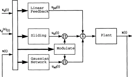
Let's consider again controlling the dynamic system represented by equation (2.3). Figure 2-1 shows the control system structure using the feedback error learning scheme. The inverse dynamics model is represented by a neural network. The total control force U(t) fed to the dynamic system is the sum of the feedback control force Uf(t) from the PD controller and the feedforward control force Ui(t) from the neural network controller.
U(t) = Uf(t) + Ui(t) (2.47)
Uf(t) = Kp(Xd(t)- X(t)) +
Kd(d(t)-X(t))
(2.48)
where Kp and Kd are feedback gains of the proportional term and the differential
term.
The inverse-dynamics model receives the desired trajectory Xd(t), and uses the feedback control force Uf(t) as the error signal to adjust its weights. The training
algorithm is the error-back propagation method developed by Rumelhart et al. [10]. As learning proceeds, the feedforward network controller will provide a greater part of the control action, while the feedback signal will gradually decrease to zero. Since the
Xd
Xd
Xd
Ui
hidden layer
Figure 2-2: Structure of a three-layer network
network receives only the desired trajectory as the input, and produces the required control force to the system, it is a representation of the nonlinear model of the inverse dynamics instead of just being a neural network version of the PD controller.
As shown in Figure 2-2, the network of the inverse dynamics model has three lay-ers. The input layer neurons represent desired trajectory, velocity, and acceleration. The output layer neurons represent the feedforward control forces.The nonlinear char-acteristics of the inverse dynamics model of the system is learned and represented by this three layered cascade of linear-weighted summation and sigmoidal nonlinearity.
Let XI, yI represent the weighted sum of the input and output of the j-th neuron
in the input layer, their relation is:
yj = Ix (2.49)
Next, let H , yH represent the weighted sum of the input and output of the k-th neuron in the hidden layer, and the weight from the j-th neuron in the input layer to the k-th neuron in the hidden layer represented by WIH, we have:
H IH 2
xCi = E
wgyJ
(2.50)Finally, the m-th neuron of the output layer is represented by z°, and y, and the
weight from the k-th neuron in the hidden layer to the m-th neuron in the output
layer is WkHO:
Xm = -- \WH Wkm °Y k (2.52)
Yo = f(xo) (2.53)
The control force output from the network is:
Uim = m (2.54)
Here, f is the widely used sigmoid function:
f(2) = 1 + (2.55)
The neuron weights are updated according to the error-back propagation method, using the feedback signal from the PD controller as the error. Let A represent the increment of weights and p be the learning rate:
AwHO
=py f(2 )u/n
(2.56)
= EW HOf(°)Ufm (2.57)
m
AWk= py j(4)&r k
(2.58)
The control command fed to the system is the sum of the feedforward force and feedback force.
Um = Uim + Uff, (2.59)
2.6 Gaussian Network Control
Another kind of neural network control method is studied with the previous con-trollers. It's called Gaussian network control, which uses a network of gaussian radial
basis functions to adaptively compensate for the plant nonlinearities [8]. The a priori information about the nonlinear function of the plant is its degree of smoothness. The weight adjustment is determined using Lyapunov theory, so the algorithm is proven to be globally stable, and the tracking errors converge to a neighborhood of zero.
Sampling theory shows that bandlimited functions can be exactly represented at a countable set of points using an appropriately chosen interpolating function. When approximation is allowed, the bandlimited restriction can be relaxed and the interpolating function gets a wider selection. Specifically, the nonlinear function f(x) can be approximated by smoothly truncated outside a compact set A so that the function can be Fourier transformed. Then by truncating the spectrum, the function
can be bandlimited and uniformly approximated by
f(x) =
E
cig,(x-
(2.60)
IEI1
where c, are the weighting coefficients and (I form a regular lattice covering the subset
AT, which is larger than the compact set A by an n-ball of radius p surrounding each point of x E A. The index set is I, = {I I E AT}.
g,(x - f) is the gaussian radial basis function given by:
g.q(x
- =
exp(-
rrlx
-
2
) exp[-7r(x-
e11
)T(x-
-)(2.61)
Here is the center of the radial gaussian, and o is a measure of its essential width. Gaussian functions are well suited for the role of interpolating function be-cause they are bounded, strictly positive and absolutely integrable, and they are their own Fourier transforms.
Expansion (2.60) maps onto a network with a single hidden layer nodes. Each node represents one term in the series with the weight
&I
connecting between theinput x and the node. It then calculates the activation energy r =
lx-
l12and outputs a gaussian function of the activation, exp(-irra-,). The output of the network is weighted summation of the output of each node, with each weight equals to c. Figure 2-3 shows the structure of the network described above.
Figure 2-3: Structure of the Gaussian network
The next step is the construction of the controller. Consider the nonlinear dy-namics system
x(-)(t) + f(x(t)) = b(x(t))u(t)
(2.62)
define the unknown nonlinear function h = b-lf, and let hA and bAl be the ra-dial gaussian network approximations to the functions h and b- 1 respectively with
approximation error h and b as small as desired on the chosen set A.
Figure 2-4 shows the structure of the control law. To guarantee the stability of the whole dynamic system, the control law is constructed as a combination of three components: a linear PD control, a sliding control and an adaptive control represented by the Gaussian network.
u(t) = -kDs(t) -
M2(x(t))llx(t)llII(t) + m(t)uol(t)
+(1
-m(t))[hA(t,x(t))
-bjA1(t,x(t))a,(t)]
(2.63)
m(t) is a modulation allowing the controller to smoothly transition between sliding and adaptive controls.
m(t) = max(O,
sat( (
))
(2.64)
Figure 2-4: Structure of the Gaussian network controller
ar(t) = ATX5(t)- )(t) (2.65)
with AT - [ 0, n-1, (n-1)An 2, ...- , (n-1)A ] and x(n)(t) is the nth derivative
of the desired trajectory.
The adaptive components hA and bAl are realized as the outputs of a single gaus-sian network, with two sets of output weights: I(t) and dI(t) for each node in the hidden layer.
A(t,x(t)) = E cI(t)9((t)- )
b'(t,x(t)) =
E
di(t)g(x(t) -
'I)(2.66)
IEIo
The output weights are adjusted according to the following adaptation law:
I(t) = -ckl[(1 -m(t))sa(t)g(x(t) -- )]
(2.67)
dI(t) = ka2 a,(t)[(1 - m(t))sa(t)g,(x(t)- HI)] (2.68)
where positive constants kal and k2 are adaptation rates. See Figure 2-3 for the detailed structure of the adaptive control law.
As proved by Sanner and Slotine in [8], when the parameters in the controller are chosen appropriately according to the a priori knowledge about the smoothness and upper bounds of the nonlinear dynamic functions, the controller thus constructed will be stable and convergent. All the states in the adaptive system will remain bounded and the tracking errors will asymptotically converge to a neighborhood of zero.
Chapter 3
Simulation on a Sensorimotor
System
In order to evaluate the performance of different controllers, a sensorimotor system is setup with a nonlinear inertia load representing the nonlinear dynamics. The detailed descriptions of the experiments are given in Chapter 4. This chapter focuses on simulations of the controller designs on a computer before implementing them on the real physical plant. This makes the process of design and analysis easy to carry out without causing physical system failures.
3.1 Nonlinear Model of the Sensorimotor Dynamic
System
The nonlinear inertia load structure is shown in Figure 3-1.A weight is attached by cable to a point on the inertia disk through a small pulley. It has a simple design easy to implement, yet the nonlinearity introduced is highly complicated as will be seen from its equation of motion, which is derived by using the Lagrange's equations.
y
L
M
Figure 3-1: Nonlinear inertia structure of the sensorimotor system
d 0OE 0£C
dt(
-
ae
(3.2)where 0 is a generalized coordinate which uniquely specifies the location of the object whose motion is being analyzed. In our case, is the angle of rotation of the load. F is the nonconservative generalized force corresponding to the generalized coordinate 0. In our case, it's the torque u applied to the load.
The kinetic energy and potential energy of the nonlinear system are
T =
-J
2+-MY2
2 2
U =Mgy
so we have
i = 1J2 + 1My2-Mgy
(3.3)
Since the relation between y and is governed by
y = vR2 + L2 _ 2RL cos 9 (3.4)
RL sin (3
we have
£
C=
JO+MyRL sin
= J + M( RL sin )2O
y
d C RL sin2 + RL sin 8 RL cos 8 RL sin 8
()
=J+ +M(
)y8 2M]
[
-
2Wt de Y Y Y Y2
[J+M(RLsin0)2] + 2M02(RL)2sin[ RL sin2 ]
Y Y2 y2
at
M[
M.[RL cos 8
8 -
RLsin .RLsin
_MgRLsinO
2
8
-Mg
y y2 Y Y
M(RL)
2sin cos
_ M (R Ls
in )32 _MgRL sin
y2 y4 y
Substituting the above expressions into the Lagrangian equation (3.2) yields
M(RL
sin
)21 . M(RL)2 sin RL sin2MgRLsin
(j
+ M yn2 ) + y2 -[cos - ]82 + = u (3.6)3.2 Simulation Results
As can be seen from equation (3.6), the dynamics of the sensorimotor system is very complex and nonlinear, thus provides a good basis for evaluating different nonlinear control methodologies. The actual parameter values of the system are
J = .002 kg m2; M = 0.4749 km; R = .0476 m; L = .177 m (3.7)
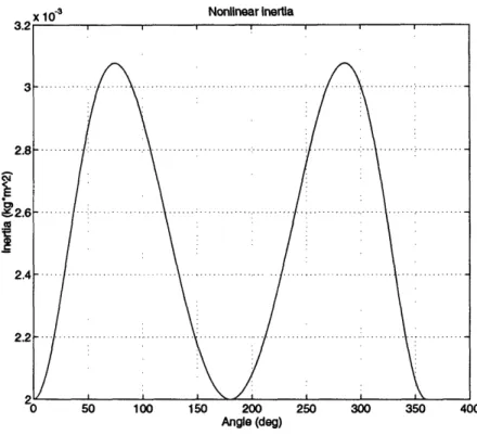
The inertia value of the load J is chosen to fall within the operating range of the sensorimotor. The dimensions of R, L and the mass of the weight M are designed to cause the variation of the system inertia to be half the value of J, as shown in Figure (3-2).
Mnnlincar inarHin
-0 50 100 150 200 250 300 350 400
Angle (deg)
Figure 3-2: Nonlinear inertia plot
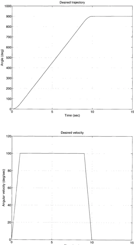
their results are compared in the following sections. To establish a fair comparison, all the controllers are designed to tracking the same trajectory shown in Figure 3-3, which is generated by a trapezoidal speed profile also shown in the same figure. The system accelerates to a constant speed and then decelerates until stops and has a duration time of 15 seconds. The closed-loop bandwidth of all controller is also the same: A = 20 hz.
3.2.1 PID Control
The control gains of the PID controller are selected according to the bandwidth A, time constant r and damping constant of the nonlinear system.
Ki = JA2/r (3.8)
Kp = J(A2r + 2(A)/r (3.9)
Kd = J(1 + 27Ar)/r
(3.10)
Desired trajectory 5 Time (sec) Desired velocity 10 0 5 10 Time (sec)
Figure 3-3: Desired trajectory and speed profile of the motion
0) a, Q) 0) 1000 900 800 700 600 500 400 300 200 100 0 0 a) §. 0) oW 15 15 l l~~~~~~~~~~~~~~~~~~~~~~~~~~~~~~~~~~~~~~~~~~~~~~~~~~~~~~~~~~~~~~~~~~~~~~~~~~~~~~~~ I -. . . I . . . . I I . . . . : . . . . 1
with
r = 1.0/(Af) (3.11)
where rf is the time constant factor.
In the simulation, the constant values are chosen as rf = 0.1 and
C
= 0.707. The duration of the motion is 15 seconds with a time step of .0005 seconds.Thus the control law for the PID controller is
u
= K
dt +
+Kp
+ KdO
(3.12)
The simulation results of the PID controller are shown from Figure 4 to Figure
3-5.
3.2.2
Sliding Control
To use the sliding method described in Chapter 2, the dynamic function (3.6) can be written as
a
= f + bu (3.13)where
b
=(J+
M(RLsinO)
(3.14)
(RL) 2 sin RL sin2 Mg RL sin
f
=-b( M(R)2
sin[cos ]2 + MR sin (3.15)Assuming the exact values of J, M, R and L are not known, thus the exact values of the control gain b and the nonlinear function f are unknown, but have a priori bounds as:
325 < b < 500 (3.16)
Tracking error
Time (sec)
Velocity error
5
Time (sec)
Figure 3-4: Tracking error and velocity error for PID control
oz, a) 0 C C 5
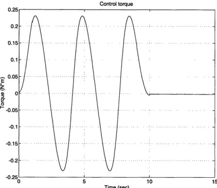
Control torque E o I--5 Time (sec)
Figure 3-5: Control torque for PID control The estimated values of b and f are
b = /bmabmin = 400 (3.18)
f
= -72sinO (3.19)and, accordingly,
fi
= V/bma,./bm = 1.25 (3.20)If-fl
< F=25
(3.21)
Defining s as s = 0 + A, computing explicitly, and proceeding as described in Chapter 2, a control law satisfying the sliding condition can be derived as
The constant values are chosen as = 50 and A = 120. The total time duration is 15 seconds with a time step of .001 seconds.
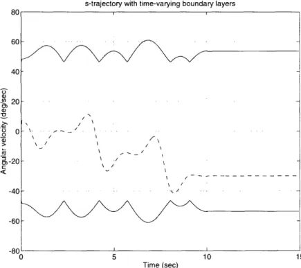
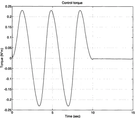
The simulation results of the sliding controller are shown from Figure 3-6 to Fig-ure 3-8.
3.2.3 Adaptive Sliding Control
The case for the adaptive sliding controller is similar to the sliding control simulation, except that the value of b is updated in each step of the control according to the following adaptation law:
b = b2n[u* + vsat(s/)]s (3.23)
with
u* = -
+ AO
(3.24)
and a constant b2 = .00005 to control the adaptation rate.
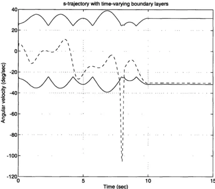
The simulation results of the adaptive sliding controller are shown from Figure 3-9 to Figure 3-12.
3.2.4 Feedback Error Learning Control
The network consists of 3 input neurons corresponding to desired displacement ad,
velocity ad and acceleration 0d, 15 neurons in the middle layer and 1 output neuron which is the feedforward control torque. Each neuron has a bias term in its weights. The starting initial weights are randomly selected between 0 and 1.
The inverse-dynamics model is acquired by repetitively experiencing the single movement pattern, while receiving the desired trajectory and monitoring the feedback control value as the error signal. The desired movement trajectory is the same as before, shown in Figure 3-3. The movement has a duration time of 15 seconds and the sampling time is 0.006 second. So the weights are adjusted 2500 times for each
Tracking error 0 5 10 15 Time (sec) Velocity error o 5 u 15b Time (sec)
Figure 3-6: Tracking error and velocity error for sliding control
0 -9 0) CD C 4:
s-trajectory with time-varying boundary layers
5
Time (sec)
10 15
Figure 3-7: Boundary layers (solid lines) and s trajectory (dashed line) for sliding control Control torque E) I-0 Time (sec)
Figure 3-8: Control torque for sliding control
60 40 2) ,0 M-20 -40 -60 / ~~~~~/ \ / l . . .. I\ I/ I I / I~~~~~~~ . 1 0 80 r , J vv 5
Tracking error 0.1 0 -0.1 -0.2 03 ¥-0.3 C--0.4 -0.5 -0.6 -0.7 , o 0 CU -v.oC-uo 5 Time (sec) Velocity error 10 15 5 Time (sec)
Figure 3-9: Tracking error and velocity error for adaptive sliding control
.
... :...
... . . ... .. . .. . . i... ....
,... . ... . . .... . .... ... .. . . .. . .......
. . ..
. . ,.. ... .. . ... . ... . . . . .. ... I .. I I , _ D ,, , -. 1 . ... .. ... ... ... . is-trajectory with time-varying boundary layers
Time (sec)
Figure 3-10: Boundary layers (solid lines) and sliding control
s trajectory (dashed line) for adaptive
Estimate of inertia b 350 F300 E 0) a) C250 200 5 Time (sec) 10 15
Figure 3-11: Inertia estimation for adaptive sliding control xs0e -o4) R0 0 so M la cm 4UU \ ?' n | !,V 5 - -··-- .. . - - .... - ...··· ···· .. ... I... ... :... ... ...· 1'-'-·--...
Control torque E z 0 I-5 Time (sec)
Figure 3-12: Control torque for adaptive sliding control each iteration according to the performance of the last iteration.
In the simulation, the learning rate and momentum term are both chosen to be 0.01 for the first 4 iterations. Then they are decreased to .008 for the rest 6 iterations. The network with 15 units in the hidden layer converges. For a smaller number of hidden units, the convergence error is bigger, while for larger number of hidden units, the model behaves unstable and is difficult to converge.
Figure 3-13 to Figure 3-19 are the results from the feedback error learning control. Figure 3-13 and Figure 3-14 show the trajectory and velocity following errors after learning. As shown in Figure 3-15 and Figure 3-16, the performance improves a lot compared to the PID controller. The control force information is shown in Figure 3-17 to Figure 3-19. The feedback control force dominates when the learning just begins. The neural network quickly learns the inverse dynamics of the vehicle during the iteration, it takes the place of the feedback as a main controller and produces a majority of the control action.
a) 0) Cv _. x 103 Tracking error Time (sec) 5
Figure 3-13: Tracking error for feedback error learning control
Velocity error 0.1 0.05 0 -0.05 -0.1 -0.15 Time (sec) 10 15
Figure 3-14: Velocity error for feedback error learning control
laU (D U) 0) 0 'ao 0) C ~JI 15 ,, l I. iF i ... . . ... ... . ... :.. ... .. . ... ...
Tracking errors from PID and NNT
Time (sec)
Figure 3-15: Comparison of tracking errors for error learning control (solid line)
Velocity errors from P[
-6M 0 -o.) 0 0) la 4: cm =r Time (sec)
Figure 3-16: Comparison of velocity error for error learning control (solid line)
PID control (dashed line) and feedback
) and NNT
5
PID control (dashed line) and feedback
EE
e
0
Time (sec)
Figure 3-17: Feedback PID control torque for feedback error learning control
Feedforward NNT control torque
E
0
I-Time (sec)
Figure 3-18: Feedforward network control torque for feedback error learning control
Control torque from PID, NNT and total torque EE e 0 5 Time (sec)
Figure 3-19: Control torque from PID (dashed line), network (dotted line) and total torque (solid line) for feedback error learning control
Phase space portrait of desired trajectories 1
0 100 200 300 400 500 600 700 800 xl
Figure 3-20: Phase space portrait of the desired trajectory
3.2.5
Gaussian Network Control
Figure 3-20 shows the phase space plot of the desired position and velocity, which is the same as used in the other controllers for the fair comparison purpose. The set Ad is thus chosen to be:
IIxIIw = max( 61 , 50l) (3.25) with its center at xo = [360, 5 0]T. This represents a rectangular subset of the state
space, Ad = [0, 720] x [0, 100]. The transition region between adaptive and sliding control modes is = 0.1 as the value in equation (2.64). So we have
A = {x I IIx - xollw < 1.1} (3.26)
The maximum desired acceleration is I3dlma < 100 as shown in the desired
tra-jectory plot in Figure 3-3 , which sets al < 42 for all x E A and the error bound to be c, = h + 4 2eb.
To achieve asymptotic tracking accuracy of 0.5 degrees, taking kD = A = 2 requires that E, < 0.3. Assuming the frequency contents of h and b-l on A are Pi = 2.5 and = 2.5 with uniform error no worse than 0.001 and an upper bound of 120 for the transform of h and 0.03 for the transform of b-l, a close following to the parameter selection procedure in [8] shows that the choices O8, = 8O = 2 and I, = 4l = 5 should be sufficient to ensure the required bound on c,. This leads to a network of gaussian nodes with variances a2 = o = 20 and mesh sizes AZ = A = 0.1. So the network includes all the nodes contained in the set AT = [-5A,, 131LA] x [-5A,23Aj], for a total of 3973 nodes.
The control laws are given by equation (2.63) and (2.66) in Chapter 2, using a value of = 0.02 as the sliding controller boundary layer, with adaptation rates
k, = ka2 = 200. Assuming uniform upper bounds of Mo(x) = 2.5, Ml(x) = .003 and
M2(x) = 0.005, the sliding controller gains are taken as k,l = 2.5 + 0.0031ai1.
Using Fourier transformation, it's easy to find that the above spectra assumptions are justified for both h and b- 1. The simulation results are shown from Figure 3-21 to Figure 3-25.
3.3 Comparison of Simulation Results
Comparison are made about a priori information requirements, closed-loop band-width, speed of convergence, memory size, control effort, computation load, and
tracking performance of these five controllers.
The PID controller needs little information about the nonlinearity, instead it re-quires a rough estimate of the inertia of the system. For the sensorimotor system, the constant inertia value J = .002 kg . m2 is used. It then selects the control gains
based on the closed-loop bandwidth and this inertia value. The tracking performance is shown to be good and the bandwidth can reach to 20 hz. The memory size is small and the computation is fast.
The sliding controller is provided with the estimated structure of the nonlinearities and the error bounds. The tracking error is slightly larger than PID controller due
Tracking error and boundaries -0 e ID tM Figure 3-21: Tracking network control 0 -0.5 0 O -1.5 Co c -2 C -2.5 -3 Time (sec)
error (solid line) and boundaries (dashed lines) for Gaussian
Velocity error -I - - I i ·.. 1 2 3 4 5 Time (sec 6 7 8 9 10 c)
Figure 3-22: Velocity error for Gaussian network control
U.5 I 0 . .. . . ... . . .. . . . .. . . . . . . ... ... :, .. :... .. ... . . . . . . . . I . . ... :... . .. . . . .:... F i .... ...:...:...:...I...:... - -L--... i _a . 0 ..
Control torques from PD, GSN and total torque E cEr 0 o I-Time (sec)
Figure 3-23: Control torque from PD (dashed line), Gaussian network (dotted line) and total torque (solid line) for Gaussian network control
Modulation m(t)
Time (sec)
Figure 3-24: Modulation for Gaussian network control
Control torques from PD and GSN zE a) a 0 2-0.01 0.02 0.03 0.04 0.05 0.06 0.07 0.08 0.09 0.1 Time (sec)
Figure 3-25: Control torque from PD (dashed line) and Gaussian network (solid line) during the early learning period of the Gaussian network control
to the large estimation error bounds. It also reaches a high closed-loop bandwidth of 20 hz and needs a slightly more computation time than PID. Unlike PID controller, the performance of sliding controller can be increased given better nonlinearity esti-mation. There is a quantified relationship between the performance and uncertainty trade off given by equation (2.35).
Adaptive sliding control has the capability to quickly learn and adapt to parameter uncertainties. Although it requires slightly more memory for adaptation, the tracking performance improves a lot after the parameters adapt to their real values. Its closed-loop bandwidth is also the same as the sliding controller. Both sliding control and adaptive sliding control are theoretically proven to be stable. So the overall system stability is assured.
While previous control techniques may fail to achieve the desired performance in the presence of unmodeled dynamics, the advantage of using a neural network for the nonlinear control is that it doesn't require any information about the nonlinear dynamics which is difficult to obtain. Its performance is much better than the above three controllers after learning. Yet the computations time is long, with control step of 0.006 seconds. Moreover, there is no theory to provide information about the structure of the network, i.e., the number of the layers and number of nodes within each layer. The numbers chosen are reached only from trail and error. There is either no theory developed regarding to the stability of the system.
Gaussian network control has precisely what the error backpropagation network needs, a systematic approach to choose the structure of the network while assuring the overall system stability. Its performance is good compared to the first three controllers and the system adapts much more quickly than the previous network. As shown in Figure 3-25, the adaptive control law takes most of the control action shortly after the first 0.05 seconds. The knowledge required for the controller is estimation of the frequency contents of the nonlinear function to be approximated. The structure of the Gaussian network is chosen based on this knowledge and the required performance. More work should be continued to study on reducing the size of the network and achieving fast computation while maintaining the desired performance.
Chapter 4
Experimental Comparison and
Results
The best way to compare different controllers is to implement them on a real physical system and evaluate their performances. The system chosen for this thesis research is a sensorimotor system manufactured by the Seiberco Inc. Sensorimotors have an extremely simple and compact design. Unlike conventional DC brushless motors, the sensorimotor provides rotor position and velocity feedback without the use of hall effect devices, encoders, or resolvers. This feedback can easily be used to develop different controllers without introducing other sensors and devices.
According to Seiberco, the inherent position feedback information is derived from the permeance variation within the permanent magnet rotor and wound stator air gap. This position information is identical to that of a brushless resolver that outputs two sinusoidal signals phase shifted 90 degrees from each other.
The motors are frameless, i.e., the stator and rotor are provided without bearings or housings. They represent a compromise between direct drive, and small, high speed motors. The laminated stator has 24 windings, of which 4 are used for sensing and the others for power. The rotor is composed of 18 samarium-cobalt magnets epoxeid to a cold-rolled steel core. The magnets are skewed to reduce torque ripple. The skewing does reduce torque output by roughly 10% when compared to a motor without a skewed rotor, but nonetheless, the high energy rare earth magnets give the